q-Generalized Tangent Based Hybrid Polynomials

Abstract

In this paper, we incorporate two known polynomials to introduce so-called 2-variable q-generalized tangent based Apostol type Frobenius–Euler polynomials. Next we present a number of properties and formulas for these polynomials such as explicit expressions, series representations, summation formulas, addition formula, q-derivative and q-integral formulas, together with numerous particular cases of the new polynomials and their associated formulas demonstrated in two tables. Further, by using computer-aided programs (for example, Mathematica or Matlab), we draw graphs of some particular cases of the new polynomials, mainly, in order to observe in several angles how zeros of these polynomials are distributed and located. Lastly we provide numerous observations and questions which naturally arise amid the present investigation.

1. Introduction

A remarkably large number of a variety of polynomials, numbers and functions, and their generalizations and variants have been introduced and investigated, due mainly to their potential usefulness and direct applications in a wide range of research subjects (see, e.g., [1,2,3,4,5,6,7,8,9,10,11,12,13,14,15,16,17,18,19] and the references therein). Among a recent deluge of various extensions of known polynomials, numbers, functions, and newly introduced polynomials, many researchers’s particular attentions have been paid to q-analogues of polynomials, numbers, and functions (see, e.g., [7,9,10,17,19,20,21,22] and the references therein). q-Bernstein polynomials amid some discrete q-operators are presented in [20] (Chapter 2). Fractional derivatives of five elementary functions including exponential function, together with their graphs, are illustrated in [21]. Certain q-orthogonal polynomials including the little and big q-Jacobi polynomials are studied in [22] (Chapter 7). Apostol type q-Frobenius–Euler polynomials are introduced and investigated in [7]. The generalized q-Apostol-Bernoulli, q-Apostol–Euler, and q-Apostol–Genocchi polynomials in two variables and their numbers are defined and studied in [9]. q-Bernoulli, q-Euler, and q-Genocchi polynomials and their numbers are investigated in [10]. New $(p,q)$-Stirling polynomials of the second kind fitting for the $(p,q)$-analogue of Bernstein polynomials are introduced and studied in [17], which includes an extensive list of references about q-and $(p,q)$-extenstions of some known polynomials and numbers, in particular, q-and $(p,q)$-Stirling polynomials and q-and $(p,q)$-Bernstein polynomials.

Moreover, the tangent polynomials and numbers, and their diverse extensions including their q-analogues have many applications in a number of research areas such as analytic number theory and physics (see, e.g., [3,12,13,19] and the references therein). For example, a new class of q-generalized tangent-based Appell polynomials by welding 2-variable q-generalized tangent polynomials and q-Appell polynomials is introduced and investigated in [19].

In this paper, we couple the polynomials in Definitions 1 and 5 to introduce new polynomials which are called the 2-variable q-generalized tangent based Apostol type Frobenius–Euler polynomials of order $\alpha$ in the variables u and v, denoted by ${}_C{\mathcal{H}}_{n,q}^{(\alpha ,m)}(u,v;\rho ;\lambda )$, in Definition 6. Then we provide a number of properties and formulas for these polynomials such as explicit representations, series representations, summation formulas, addition formula, q-derivative, q-integral formulas, numerous particular cases of the new polynomials and their related formulas illustrated with Table 1 and Table 2. Moreover, we use computer-aided programs (for example, Mathematica or Matlab) to draw graphs of some particular cases of the new polynomials, mainly, in order to observe in several angles how zeros of these polynomials are distributed and located. Finally we give a number of observations and questions which naturally occurs amid this investigation.

Table 1. Particular cases of the ${}_C{\mathcal{H}}_{n,q}^{(\alpha ,m)}(u,v;\rho ;\lambda )$.

S. No.	Relations between the ${}_{\mathit{C}}{\mathcal{H}}_{\mathit{n},\mathit{q}}^{(\mathit{\alpha },\mathit{m})}(\mathit{u},\mathit{v};\mathit{\rho };\mathit{\lambda })$ and Its Particular Cases	Names of the Resultant q-Special Polynomials	Generating Functions of the Resultant q-Special Polynomials
I.	${}_C{\mathcal{H}}_{n,q}^{(\alpha ,m)}(u,v;-1;\lambda )={}_C{\mathcal{H}}_{n,q}^{(\alpha ,m)}(u,v;\lambda )$	q-generalized tangent-Apostol	${\left(\frac{2}{\lambda e_q\left(t\right)+1}\right)}^{\alpha }\left(\frac{2}{e_q\left(mt\right)+1}\right)e_q\left(ut\right)E_q\left(vt\right)$
		Euler polynomials (qGTAEP)	$={\sum }_{n=0}^{\infty }{}_C{\mathcal{H}}_{n,q}^{(\alpha ,m)}(u,v;\lambda )\frac{t^n}{{\left[n\right]}_q!}$
II.	${}_C{\mathcal{H}}_{n,q}^{(\alpha ,m)}(u,v;\rho ;1)={}_C{\mathcal{F}}_{n,q}^{(\alpha ,m)}(u,v;\rho )$	q-generalized tangent-Frobenius	${\left(\frac{1-\rho }{e_q\left(t\right)-\rho }\right)}^{\alpha }\left(\frac{2}{e_q\left(mt\right)+1}\right)e_q\left(ut\right)E_q\left(vt\right)$
		-Euler polynomials (qGTFEP)	$={\sum }_{n=0}^{\infty }{}_C{\mathcal{F}}_{n,q}^{(\alpha ,m)}(u,v;\rho )\frac{t^n}{{\left[n\right]}_q!}$
III.	${}_C{\mathcal{H}}_{n,q}^{(\alpha ,m)}(u,v;-1;1)={}_C{\mathcal{E}}_{n,q}^{(\alpha ,m)}(u,v)$	q-generalized tangent	${\left(\frac{2}{e_q\left(t\right)+1}\right)}^{\alpha }\left(\frac{2}{e_q\left(mt\right)+1}\right)e_q\left(ut\right)E_q\left(vt\right)$
		-Euler polynomials (qGTEP)	$={\sum }_{n=0}^{\infty }{}_C{\mathcal{E}}_{n,q}^{(\alpha ,m)}(u,v)\frac{t^n}{{\left[n\right]}_q!}$
IV.	${}_C{\mathcal{H}}_{n,q}^{(\alpha ,2)}(u,v;\rho ;\lambda )={}_T{H}_{n,q}^{\left(\alpha \right)}(u,v;\rho ;\lambda )$	q-tangent-Apostol Frobenius	${\left(\frac{1-\rho }{\lambda e_q\left(t\right)-\rho }\right)}^{\alpha }\left(\frac{2}{e_q\left(2t\right)+1}\right)e_q\left(ut\right)E_q\left(vt\right)$
		-Euler polynomials (qTAFEP)	$={\sum }_{n=0}^{\infty }{}_T{H}_{n,q}^{\left(\alpha \right)}(u,v;\rho ;\lambda )\frac{t^n}{{\left[n\right]}_q!}$
V.	${}_C{\mathcal{H}}_{n,q}^{(\alpha ,2)}(u,v;-1;\lambda )={}_T{H}_{n,q}^{\left(\alpha \right)}(u,v;\lambda )$	q-tangent-Apostol	${\left(\frac{2}{\lambda e_q\left(t\right)+1}\right)}^{\alpha }\left(\frac{2}{e_q\left(2t\right)+1}\right)e_q\left(ut\right)E_q\left(vt\right)$
		Euler polynomials (qTAEP)	$={\sum }_{n=0}^{\infty }{}_T{H}_{n,q}^{\left(\alpha \right)}(u,v;\lambda )\frac{t^n}{{\left[n\right]}_q!}$
VI.	${}_C{\mathcal{H}}_{n,q}^{(\alpha ,2)}(u,v;\rho ;1)={}_T{\mathcal{F}}_{n,q}^{\left(\alpha \right)}(u,v;\rho )$	q-tangent-Frobenius	${\left(\frac{1-\rho }{e_q\left(t\right)-\rho }\right)}^{\alpha }\left(\frac{2}{e_q\left(2t\right)+1}\right)e_q\left(ut\right)E_q\left(vt\right)$
		-Euler polynomials (qTFEP)	$={\sum }_{n=0}^{\infty }{}_T{\mathcal{F}}_{n,q}^{\left(\alpha \right)}(u,v;\rho )\frac{t^n}{{\left[n\right]}_q!}$
VII.	${}_C{\mathcal{H}}_{n,q}^{(\alpha ,2)}(u,v;-1;1)={}_T{\mathcal{E}}_{n,q}^{\left(\alpha \right)}(u,v)$	q-tangent-Euler	${\left(\frac{2}{e_q\left(t\right)+1}\right)}^{\alpha }\left(\frac{2}{e_q\left(2t\right)+1}\right)e_q\left(ut\right)E_q\left(vt\right)$
		polynomials (qTEP)	$={\sum }_{n=0}^{\infty }{}_T{\mathcal{E}}_{n,q}^{\left(\alpha \right)}(u,v)\frac{t^n}{{\left[n\right]}_q!}$
VIII.	${}_C{\mathcal{H}}_{n,q}^{(\alpha ,1)}(u,v;\rho ;\lambda )={}_{\mathcal{E}}{H}_{n,q}^{\left(\alpha \right)}(u,v;\rho ;\lambda )$	q-Euler-Apostol Frobenius	${\left(\frac{1-\rho }{\lambda e_q\left(t\right)-\rho }\right)}^{\alpha }\left(\frac{2}{e_q\left(t\right)+1}\right)e_q\left(ut\right)E_q\left(vt\right)$
		-Euler polynomials (qEAFEP)	$={\sum }_{n=0}^{\infty }{}_{\mathcal{E}}{H}_{n,q}^{\left(\alpha \right)}(u,v;\rho ;\lambda )\frac{t^n}{{\left[n\right]}_q!}$
IX.	${}_C{\mathcal{H}}_{n,q}^{(\alpha ,1)}(u,v;-1;\lambda )={}_{\mathcal{E}}{H}_{n,q}^{(\alpha ,m)}(u,v;\lambda )$	q-Euler-Apostol	${\left(\frac{2}{\lambda e_q\left(t\right)+1}\right)}^{\alpha }\left(\frac{2}{e_q\left(t\right)+1}\right)e_q\left(ut\right)E_q\left(vt\right)$
		Euler polynomials (qEAEP)	$={\sum }_{n=0}^{\infty }{}_{\mathcal{E}}{H}_{n,q}^{\left(\alpha \right)}(u,v;\lambda )\frac{t^n}{{\left[n\right]}_q!}$
X.	${}_C{\mathcal{H}}_{n,q}^{(\alpha ,1)}(u,v;\rho ;1)={}_{\mathcal{E}}{\mathcal{F}}_{n,q}^{(\alpha ,m)}(u,v;\rho )$	q-Euler-Frobenius	${\left(\frac{1-\rho }{e_q\left(t\right)-\rho }\right)}^{\alpha }\left(\frac{2}{e_q\left(t\right)+1}\right)e_q\left(ut\right)E_q\left(vt\right)$
		-Euler polynomials (qEFEP)	$={\sum }_{n=0}^{\infty }{}_{\mathcal{E}}{\mathcal{F}}_{n,q}^{\left(\alpha \right)}(u,v;\rho )\frac{t^n}{{\left[n\right]}_q!}$
XI.	${}_C{\mathcal{H}}_{n,q}^{(\alpha ,1)}(u,v;-1;1)={}_{\mathcal{E}}{\mathcal{E}}_{n,q}^{(\alpha ,m)}(u,v)$	2-iterated q-Euler	${\left(\frac{2}{e_q\left(t\right)+1}\right)}^{\alpha +1}{e}_q\left(ut\right)E_q\left(vt\right)$
		polynomials (2IqEP)	$={\sum }_{n=0}^{\infty }{}_{\mathcal{E}}{\mathcal{E}}_{n,q}^{\left(\alpha \right)}(u,v)\frac{t^n}{{\left[n\right]}_q!}$

Table 2. Corresponding results for ${}_C{\mathcal{H}}_{n,q}^{(\alpha ,m)}(u,v;\lambda )$, ${}_C{\mathcal{F}}_{n,q}^{(\alpha ,m)}(u,v;\rho )$, and ${}_C{\mathcal{E}}_{n,q}^{(\alpha ,m)}(u,v)$.

Results	${}_{\mathit{C}}{\mathcal{H}}_{\mathit{n},\mathit{q}}^{(\mathit{\alpha },\mathit{m})}(\mathit{u},\mathit{v};\mathit{\lambda })$	${}_{\mathit{C}}{\mathcal{F}}_{\mathit{n},\mathit{q}}^{(\mathit{\alpha },\mathit{m})}(\mathit{u},\mathit{v};\mathit{\rho })$	${}_{\mathit{C}}{\mathcal{E}}_{\mathit{n},\mathit{q}}^{(\mathit{\alpha },\mathit{m})}(\mathit{u},\mathit{v})$
	${}_C{\mathcal{H}}_{n,q}^{(\alpha ,m)}(u,v;\lambda )$	${}_C{\mathcal{F}}_{n,q}^{(\alpha ,m)}(u,v;\rho )$	${}_C{\mathcal{E}}_{n,q}^{(\alpha ,m)}(u,v)$
I. Series	$={\sum }_{k=0}^n{\left[\genfrac{}{}{0pt}{}{n}{k}\right]}_q{C}_{n-k,m,q}{H}_{k,q}^{\left(\alpha \right)}(u,v;\lambda )$	$={\sum }_{k=0}^n{\left[\genfrac{}{}{0pt}{}{n}{k}\right]}_q{C}_{n-k,m,q}{\mathcal{F}}_{k,q}^{\left(\alpha \right)}(u,v;\rho )$	$={\sum }_{k=0}^n{\left[\genfrac{}{}{0pt}{}{n}{k}\right]}_q{C}_{n-k,m,q}{\mathcal{E}}_{k,q}^{\left(\alpha \right)}(u,v)$
expansions
	${}_C{\mathcal{H}}_{n,q}^{(\alpha ,m)}(u,v;\lambda )$	${}_C{\mathcal{F}}_{n,q}^{(\alpha ,m)}(u,v;\rho )$	${}_C{\mathcal{E}}_{n,q}^{(\alpha ,m)}(u,v)$
	$={\sum }_{k=0}^n{\sum }_{r=0}^k{\left[\genfrac{}{}{0pt}{}{n}{k}\right]}_q{\left[\genfrac{}{}{0pt}{}{k}{r}\right]}_q$	$={\sum }_{k=0}^n{\sum }_{r=0}^k{\left[\genfrac{}{}{0pt}{}{n}{k}\right]}_q{\left[\genfrac{}{}{0pt}{}{k}{r}\right]}_q$	$={\sum }_{k=0}^n{\sum }_{r=0}^k{\left[\genfrac{}{}{0pt}{}{n}{k}\right]}_q{\left[\genfrac{}{}{0pt}{}{k}{r}\right]}_q$
	$\times q^{r(r-1)/2}{H}_{k-r,q}^{\left(\alpha \right)}\left(\lambda \right)v^r{C}_{n-k,m,q}\left(u\right)$	$\times q^{r(r-1)/2}{\mathcal{F}}_{k-r,q}^{\left(\alpha \right)}\left(\rho \right)v^r{C}_{n-k,m,q}\left(u\right)$	$\times q^{r(r-1)/2}{\mathcal{E}}_{k-r,q}^{\left(\alpha \right)}{v}^r{C}_{n-k,m,q}\left(u\right)$
	${}_C{\mathcal{H}}_{n,q}^{(\alpha ,m)}(u,v;\lambda )$	${}_C{\mathcal{F}}_{n,q}^{(\alpha ,m)}(u,v;\rho )$	${}_C{\mathcal{E}}_{n,q}^{(\alpha ,m)}(u,v)$
	$={\sum }_{k=0}^n{\left[\genfrac{}{}{0pt}{}{n}{k}\right]}_q{}_C{\mathcal{H}}_{n-k}^{(\alpha ,m)}\left(\lambda \right){(u+v)}_q^k$	$={\sum }_{k=0}^n{\left[\genfrac{}{}{0pt}{}{n}{k}\right]}_q{}_C{\mathcal{F}}_{n-k}^{(\alpha ,m)}\left(\rho \right){(u+v)}_q^k$	$={\sum }_{k=0}^n{\left[\genfrac{}{}{0pt}{}{n}{k}\right]}_q{}_C{\mathcal{E}}_{n-k}^{(\alpha ,m)}{(u+v)}_q^k$
II. Summation	${}_C{\mathcal{H}}_{n,q}^{(\alpha ,m)}(u,v;\lambda )$	${}_C{\mathcal{F}}_{n,q}^{(\alpha ,m)}(u,v;\rho )$	${}_C{\mathcal{E}}_{n,q}^{(\alpha ,m)}(u,v)$
Formulae	$={\sum }_{k=0}^n{\left[\genfrac{}{}{0pt}{}{n}{k}\right]}_q{}_C{\mathcal{H}}_{n-k}^{(\alpha ,m)}(0,v;\lambda )u^k$	$={\sum }_{k=0}^n{\left[\genfrac{}{}{0pt}{}{n}{k}\right]}_q{}_C{\mathcal{F}}_{n-k}^{(\alpha ,m)}(0,v;\rho )u^k$	$={\sum }_{k=0}^n{\left[\genfrac{}{}{0pt}{}{n}{k}\right]}_q{}_C{\mathcal{E}}_{n-k}^{(\alpha ,m)}(0,v)u^k$
	${}_C{\mathcal{H}}_{n,q}^{(\alpha ,m)}(u,v;\lambda )$	${}_C{\mathcal{F}}_{n,q}^{(\alpha ,m)}(u,v;\rho )$	${}_C{\mathcal{E}}_{n,q}^{(\alpha ,m)}(u,v)$
	$={\sum }_{k=0}^n{\left[\genfrac{}{}{0pt}{}{n}{k}\right]}_q{}_C{\mathcal{H}}_{n-k}^{(\alpha ,m)}(u,0;\lambda )v^k$	$={\sum }_{k=0}^n{\left[\genfrac{}{}{0pt}{}{n}{k}\right]}_q{}_C{\mathcal{F}}_{n-k}^{(\alpha ,m)}(u,0,\rho )v^k$	$={\sum }_{k=0}^n{\left[\genfrac{}{}{0pt}{}{n}{k}\right]}_q{}_C{\mathcal{E}}_{n-k}^{(\alpha ,m)}(u,0)v^k$

2. Preliminaries

In this section, we recall certain standard notations for q-analogues (or extensions), definitions, and some required properties (see, e.g., [22,23,24,25,26,27,28]), together with a remark.

The q-analogues of a number $a\in \mathbb{C}$ and the factorial $n!$ are given, respectively, by

$${\left[a\right]}_q=\frac{1-q^a}{1-q}(q\in \mathbb{C}\backslash \left\{1\right\}),$$

(1)

and

$${\left[n\right]}_q!=\prod _{m=1}^n{\left[m\right]}_q={\left[1\right]}_q{\left[2\right]}_q{\left[3\right]}_q\cdots {\left[n\right]}_q(n\in \mathbb{N}),{\left[0\right]}_q!:=1.$$

(2)

Here and in the following, let $\mathbb{C}$, $\mathbb{R}$, ${\mathbb{R}}^{+}$, $\mathbb{Z}$, and $\mathbb{N}$ denote the sets of complex numbers, real numbers, positive real numbers, integers, and positive integers, respectively, and let ${\mathbb{N}}_0:=\mathbb{N}\cup \left\{0\right\}$. The q-binomial coefficient ${\left[\genfrac{}{}{0pt}{}{n}{k}\right]}_q$ is defined by (see, e.g., [23] (p. 484))

$${\left[\genfrac{}{}{0pt}{}{n}{k}\right]}_q:=\frac{{\left[n\right]}_q!}{{\left[k\right]}_q!{[n-k]}_q!}=\frac{{(q;q)}_n}{{(q;q)}_k{(q;q)}_{n-k}}={\left[\genfrac{}{}{0pt}{}{n}{n-k}\right]}_q\left(n\in {\mathbb{N}}_0,k=0,1,2,\dots ,n\right).$$

(3)

Here ${(a;q)}_n$ is the q-shifted factorial defined by (see, e.g., [22,23,26,28])

$${(a;q)}_n:=\left\{\begin{array}{cc}1\hfill & (n=0),\hfill \\ {\displaystyle \prod _{k=0}^{n-1}}\left(1-a{q}^k\right)\hfill & (n\in \mathbb{N}),\hfill \end{array}\right.$$

(4)

where $a,q\in \mathbb{C}$ and it is assumed that $a\ne q^{-m}$$\left(m\in {\mathbb{N}}_0\right)$. We also recall

$${(a;q)}_{\infty }:=\prod _{k=0}^{\infty }\left(1-a{q}^k\right)\left(a,q\in \mathbb{C},\left|q\right|<1\right).$$

(5)

The q-analogue of the binomial expansion is given by (see, e.g., [23] (p. 484), [9] (Equation (4)))

$${(u+v)}_q^n=\sum _{k=0}^n{\left[\genfrac{}{}{0pt}{}{n}{k}\right]}_q{q}^{k(k-1)/2}{u}^{n-k}{v}^k\left(n\in {\mathbb{N}}_0,u,v\in \mathbb{C}\right).$$

(6)

Recall two q-exponential functions (see, e.g., [23] (p. 492), [9] (Equations (6) and (7)), [28] (p. 488))

$$e_q\left(u\right)=\sum _{k=0}^{\infty }\frac{u^k}{{\left[k\right]}_q!}\left({0<\left|q\right|<1,\left|u\right|<|1-q|}^{-1}\right),$$

(7)

and

$$E_q\left(u\right)=\sum _{k=0}^{\infty }{q}^{k(k-1)/2}\frac{u^k}{{\left[k\right]}_q!}\left(0<\left|q\right|<1,u\in \mathbb{C}\right).$$

(8)

They satisfy the following relation

$$e_q\left(t\right)E_q(-t)=e_q(-t)E_q\left(t\right)=1.$$

(9)

The relation (9) can be proved by using the following Euler’s formulae (see, e.g., [23] (p. 490), [9] (Equations (6) and (7)), [28] (p. 487)):

$$\sum _{n=0}^{\infty }\frac{z^n}{{(q;q)}_n}=\frac{1}{{(z;q)}_{\infty }}\left(\left|q\right|<1,\left|z\right|<1\right)$$

(10)

and

$$\sum _{n=0}^{\infty }\frac{{(-1)}^n{q}^{\left(\genfrac{}{}{0pt}{}{n}{2}\right)}{z}^n}{{(q;q)}_n}={(z;q)}_{\infty }\left(\left|q\right|<1,z\in \mathbb{C}\right).$$

(11)

F. H. Jackson [29] may be recognized as the first researcher to develop q-calculus in a systematic way. The q-derivative of a function $f\left(t\right)$ is defined by

$$D_q\left\{f\left(t\right)\right\}:=\frac{d_{q}f\left(t\right)}{d_{q}t}=\frac{f\left(qt\right)-f\left(t\right)}{(q-1)t}.$$

(12)

Obviously

$$\underset{q\to 1}{lim}{D}_q\left\{f\left(t\right)\right\}=\frac{d}{dt}\left\{f\left(t\right)\right\},$$

if $f\left(t\right)$ is differentiable. The q-derivative of functions $e_q\left(u\right)$ and $E_q\left(u\right)$ with respect to u are given by

$$D_{q,u}{e}_q\left(ut\right)=t{e}_q\left(ut\right),D_{q,u}{E}_q\left(ut\right)=t{E}_q\left(qut\right).$$

(13)

Here and throughout, $D_{q,u}$ denotes the q-derivative of a function of several variables with respect to u. The following q-derivative formulas for product and quotient of functions $f\left(u\right)$ and $g\left(u\right)$ are satisfied:

$$D_q\left(f\left(u\right)g\left(u\right)\right)=f\left(qu\right)D_{q}g\left(u\right)+g\left(u\right)D_{q}f\left(u\right)=f\left(u\right)D_{q}g\left(u\right)+g\left(qu\right)D_{q}f\left(u\right),$$

(14)

and

$$D_q\left(\frac{f\left(u\right)}{g\left(u\right)}\right)=\frac{g\left(qu\right)D_{q}f\left(u\right)-f\left(qu\right)D_{q}g\left(u\right)}{g\left(u\right)g\left(qu\right)}=\frac{g\left(u\right)D_{q}f\left(u\right)-f\left(u\right)D_{q}g\left(u\right)}{g\left(u\right)g\left(qu\right)}.$$

(15)

Suppose that $0\le a<b<\infty$. The (Jackson’s) definite q-integral is defined as follows (see, e.g., [26] (Section 19), [28] (Chapter 6)), [29]:

$${\int }_0^{b}f\left(t\right)d_{q}t=(1-q)\sum _{j=0}^{\infty }{q}^{j}bf\left(q^{j}b\right)$$

(16)

and

$${\int }_a^{b}f\left(t\right)d_{q}t={\int }_0^{b}f\left(t\right)d_{q}t-{\int }_0^{a}f\left(t\right)d_{q}t.$$

(17)

A fundamental theorem of q-calculus is recalled as in the following lemma (see, e.g., [26] (p. 74, Corollary 20.1)).

Lemma 1.

If $f^{\prime }\left(t\right)$ exists in a neighborhood of $t=0$ and is continuous at $t=0$, where $f^{\prime }\left(t\right)$ denotes the ordinary derivative of $f\left(t\right)$, we have

$${\int }_a^b{D}_{q}f\left(t\right)d_{q}t=f\left(b\right)-f\left(a\right),$$

(18)

where $0\le a<b<\infty$.

We recall the q-generalized tangent polynomials and numbers in [18] (Definition 2.1) whose restrictions may be slightly amended as in the following definition.

Definition 1.

(cf. [18]) The q-generalized tangent polynomials $C_{n,m,q}\left(u\right)$ in the variable u(abbreviated as $qGTP$) are defined by means of the generating function

$$\left(\frac{2}{e_q\left(mt\right)+1}\right)e_q\left(ut\right)=\sum _{n=0}^{\infty }{C}_{n,m,q}\left(u\right)\frac{t^n}{{\left[n\right]}_q!}$$

(19)

$$\left(q,u\in \mathbb{C},m\in {\mathbb{R}}^{+}{,0<\left|q\right|<1,max\left\{\right|ut|,|mt\left|\right\}<|1-q|}^{-1},\left|t\right|<\xi \right).$$

Here ξ is the smallest one among the absolute values of all complex zeros of $e_q\left(mt\right)+1=0$. The cases $C_{n,m,q}:=C_{n,m,q}\left(0\right)$ are called q-generalized tangent numbers.

Note that the following two particular cases

$$\underset{m\to 1}{lim}{C}_{n,m,q}\left(u\right)={\mathcal{E}}_{n,q}\left(u\right)$$

(20)

and

$$\underset{m\to 2}{lim}{C}_{n,m,q}\left(u\right)=T_{n,q}\left(u\right)$$

(21)

are called q-Euler polynomials (see [16]) and q-tangent polynomials (see [12]), respectively.

Further the q-Apostol-Bernoulli polynomials, q-Apostol–Euler polynomials, q-Apostol–Genocchi polynomials, and Apostol-type q-Frobenius–Euler polynomials have recently been actively introduced and investigated (see, e.g., [2,7,8,9,14,15,16] and the references therein). They are recalled in the following definitions.

Definition 2.

(see [9]) The q-Apostol-Bernoulli polynomials ${\mathfrak{B}}_{n,q}^{\left(\alpha \right)}(u,v;\lambda )$ of order α in variables u and v(abbreviated as $qABP$) are defined by means of the generating function

$${\left(\frac{t}{\lambda e_q\left(t\right)-1}\right)}^{\alpha }{e}_q\left(ut\right)E_q\left(vt\right)=\sum _{n=0}^{\infty }{\mathfrak{B}}_{n,q}^{\left(\alpha \right)}(u,v;\lambda )\frac{t^n}{{\left[n\right]}_q!}$$

(22)

$$\left(q,u,v\in \mathbb{C},\alpha \in \mathbb{N},0<\left|q\right|<1,|t+log\lambda |<2\pi \right).$$

Here ${\mathfrak{B}}_{n,q}^{\left(\alpha \right)}\left(\lambda \right):={\mathfrak{B}}_{n,q}^{\left(\alpha \right)}(0,0;\lambda )$ are called the q-Apostol-Bernoulli numbers.

Definition 3.

(see [9]) The q-Apostol–Euler polynomials ${\mathfrak{E}}_{n,q}^{\left(\alpha \right)}(u,v;\lambda )$ of order α in variables u and v(abbreviated as $qAEP$) are defined by means of the generating function

$${\left(\frac{2}{\lambda e_q\left(t\right)+1}\right)}^{\alpha }{e}_q\left(ut\right)E_q\left(vt\right)=\sum _{n=0}^{\infty }{\mathfrak{E}}_{n,q}^{\left(\alpha \right)}(u,v;\lambda )\frac{t^n}{{\left[n\right]}_q!}$$

(23)

$$\left(q,u,v\in \mathbb{C},\alpha \in \mathbb{N},0<\left|q\right|<1,|t+log(-\lambda \left)\right|<\pi \right).$$

Here ${\mathfrak{E}}_{n,q}^{\left(\alpha \right)}\left(\lambda \right):={\mathfrak{E}}_{n,q}^{\left(\alpha \right)}(0,0;\lambda )$ are called the q-Apostol–Euler numbers.

Definition 4.

(see [9]) The q-Apostol–Genocchi polynomials ${\mathcal{G}}_{n,q}^{\left(\alpha \right)}(u,v;\lambda )$ of order α in variables u and v (abbreviated as $qAGP$) are defined by means of the generating function

$${\left(\frac{2t}{\lambda e_q\left(t\right)+1}\right)}^{\alpha }{e}_q\left(ut\right)E_q\left(vt\right)=\sum _{n=0}^{\infty }{\mathcal{G}}_{n,q}^{\left(\alpha \right)}(u,v;\lambda )\frac{t^n}{{\left[n\right]}_q!}$$

(24)

$$\left(q,u,v\in \mathbb{C},\alpha \in \mathbb{N},0<\left|q\right|<1,|t+log(-\lambda \left)\right|<\pi \right).$$

Here ${\mathcal{G}}_{n,q}^{\left(\alpha \right)}\left(\lambda \right):={\mathcal{G}}_{n,q}^{\left(\alpha \right)}(0,0;\lambda )$ are called the q-Apostol–Genocchi numbers.

Definition 5.

(see [7]) The Apostol type q-Frobenius–Euler polynomials $H_{n,q}^{\left(\alpha \right)}(u,v;\rho ;\lambda )$ of order α in the variables u and v (abbreviated as $ATqFEP$) are defined by means of the generating function

$${\left(\frac{1-\rho }{\lambda e_q\left(t\right)-\rho }\right)}^{\alpha }{e}_q\left(ut\right)E_q\left(vt\right)=\sum _{n=0}^{\infty }{H}_{n,q}^{\left(\alpha \right)}(u,v;\rho ;\lambda )\frac{t^n}{{\left[n\right]}_q!}$$

(25)

$$\left(q,\lambda ,\rho ,u,v\in \mathbb{C},\alpha \in \mathbb{N},|<1,0<|q|<1,\rho \ne 1,|\lambda /\rho |<1\right).$$

Here the Apostol type q-Frobenius–Euler numbers $H_{n,q}^{\left(\alpha \right)}(\rho ;\lambda ):=H_{n,q}^{\left(\alpha \right)}(0,0;\rho ;\lambda )$ of order α are defined by

$${\left(\frac{1-\rho }{\lambda e_q\left(t\right)-\rho }\right)}^{\alpha }=\sum _{n=0}^{\infty }{H}_{n,q}^{\left(\alpha \right)}(\rho ;\lambda )\frac{t^n}{{\left[n\right]}_q!}$$

(26)

$$\left(q,\lambda ,\rho \in \mathbb{C},\alpha \in \mathbb{N},|<1,0<|q|<1,\rho \ne 1,|\lambda /\rho |<1\right).$$

Remark 1.

The constraints in Definitions 2–5 should and can be modified as those in Definition 6 (see also Definition 1).

The polynomials $H_{n,q}^{\left(\alpha \right)}(u,v;\rho ;\lambda )$ in Definition 5 are found to reduce to yield

• $H_{n,q}^{\left(\alpha \right)}(u,v;-1;\lambda )=H_{n,q}^{\left(\alpha \right)}(u,v;\lambda )$ (q-Apostol Euler polynomials [7]);
• $H_{n,q}^{\left(\alpha \right)}(u,v;\rho ;1)={\mathcal{F}}_{n,q}^{\left(\alpha \right)}(u;v;\rho )$ (q-Frobenius–Euler polynomials [14,15]);
• $H_{n,q}^{\left(\alpha \right)}(u,v;-1;1)={\mathcal{E}}_{n,q}^{\left(\alpha \right)}(u,v)$ (q-Euler polynomials [8]);
• $H_{n,q}^{\left(\alpha \right)}(u,0;\rho ;\lambda )=H_{n,q}^{\left(\alpha \right)}(u;\rho ;\lambda )$ (q-Apostol type Frobenius–Euler polynomials [16]);
• $\underset{q\to 1^{-}}{lim}{H}_{n,q}^{\left(\alpha \right)}(u,0;\rho ;\lambda )=H_n^{\left(\alpha \right)}(u;\rho ;\lambda )$ (Apostol type Frobenius–Euler polynomials [2]).
  The five above-right-hand sided polynomials when $\alpha =1$ are simply written as follows:

  $$\begin{gathered} H_{n,q}^{\left(1\right)}(u,v;\lambda ):=H_{n,q}(u,v;\lambda ); \\ {\mathcal{F}}_{n,q}^{\left(1\right)}(u;v;\rho ):={\mathcal{F}}_{n,q}(u;v;\rho ); \\ {\mathcal{E}}_{n,q}^{\left(1\right)}(u,v):={\mathcal{E}}_{n,q}(u,v); \\ {H}_{n,q}^{\left(1\right)}(u;\rho ;\lambda ):=H_{n,q}(u;\rho ;\lambda ); \\ {H}_n^{\left(1\right)}(u;\rho ;\lambda ):=H_n(u;\rho ;\lambda ). \end{gathered}$$

3. q-Generalized Tangent-Apostol Type Frobenius–Euler Polynomials and Their Related Formulas

In this section, we introduce the q-generalized tangent based Apostol type Frobenius–Euler polynomials ${}_C{\mathcal{H}}_{n,q}^{(\alpha ,m)}(u,v;\rho ;\lambda )$ and investigate some of their properties.

Definition 6.

The 2-variable q-generalized tangent based Apostol type Frobenius–Euler polynomials ${}_C{\mathcal{H}}_{n,q}^{(\alpha ,m)}(u,v;\rho ;\lambda )$ of order α in the variables u and v (abbreviated as $qGTATFEP$) are defined by means of the following generating function

$${\left(\frac{1-\rho }{\lambda e_q\left(t\right)-\rho }\right)}^{\alpha }\left(\frac{2}{e_q\left(mt\right)+1}\right)e_q\left(ut\right)E_q\left(vt\right)=\sum _{n=0}^{\infty }{}_C{\mathcal{H}}_{n,q}^{(\alpha ,m)}(u,v;\rho ;\lambda )\frac{t^n}{{\left[n\right]}_q!}$$

(27)

$$\begin{gathered} \left(\alpha \in \mathbb{N},m\in {\mathbb{R}}^{+},u,v,q\in \mathbb{C},\rho \in \mathbb{C}\backslash \left\{1\right\},\lambda \in \mathbb{C}\backslash \left\{0\right\},\lambda \ne {\rho , \\ 0<\left|q\right|<1,\left|ut\right|<|1-q|}^{-1},\left|t\right|<min\{\xi /m,\eta \}\right), \end{gathered}$$

(28)

where ξ is the same as in the restrictions of Definition 1 and η is the smallest nonzero one among the absolute values of all complex zeros of $e_q\left(t\right)-\rho /\lambda =0$. Here

$${}_C{\mathcal{H}}_{n,q}^{(\alpha ,m)}(\rho ;\lambda ):={}_C{\mathcal{H}}_{n,q}^{(\alpha ,m)}(0,0;\rho ;\lambda )$$

(29)

are called the q-generalized tangent-Apostol type Frobenius–Euler numbers of order α.

By selecting suitable parameters in generating function (27), we obtain several members belonging to the family of qGTATFEP ${}_C{\mathcal{H}}_{n,q}^{(\alpha ,m)}(u,v;\rho ;\lambda )$, which are listed in Table 1.

For simplicity, let

$${\mathcal{G}}_q(\alpha ,m;u,v;\rho ;\lambda ):={\left(\frac{1-\rho }{\lambda e_q\left(t\right)-\rho }\right)}^{\alpha }\left(\frac{2}{e_q\left(mt\right)+1}\right)e_q\left(ut\right)E_q\left(vt\right)$$

(30)

be the generating function in (27).

We present two series representations for the polynomials $qGTATFEP$ by using series manipulation techniques in some combinations of the polynomials and numbers in Section 1 as in the following theorem.

Theorem 1.

Let $n\in {\mathbb{N}}_0$. Moreover, let the other parameters and variables in the identities below be assumed to satisfy the restrictions (28). Then

$${}_C{\mathcal{H}}_{n,q}^{(\alpha ,m)}(u,v;\rho ;\lambda )=\sum _{k=0}^n{\left[\genfrac{}{}{0pt}{}{n}{k}\right]}_q{C}_{n-k,m,q}{H}_{k,q}^{\left(\alpha \right)}(u,v;\rho ;\lambda ),$$

(31)

and

$${}_C{\mathcal{H}}_{n,q}^{(\alpha ,m)}(u,v;\rho ;\lambda )=\sum _{k=0}^n\sum _{r=0}^k{\left[\genfrac{}{}{0pt}{}{n}{k}\right]}_q{\left[\genfrac{}{}{0pt}{}{k}{r}\right]}_q{q}^{r(r-1)/2}{H}_{k-r,q}^{\left(\alpha \right)}(\rho ;\lambda )v^r{C}_{n-k,m,q}\left(u\right).$$

(32)

Proof. 

We find from (27) and (30) that

$$\begin{array}{cc}{\mathcal{G}}_q(\alpha ,m;u,v;\rho ;\lambda )& =\left(\frac{2}{e_q\left(mt\right)+1}\right)·{\left(\frac{1-\rho }{\lambda e_q\left(t\right)-\rho }\right)}^{\alpha }{e}_q\left(ut\right)E_q\left(vt\right)\hfill \\ & ={\displaystyle \sum _{n=0}^{\infty }}{C}_{n,m,q}\frac{t^n}{{\left[n\right]}_q!}·{\displaystyle \sum _{k=0}^{\infty }}{H}_{k,q}^{\left(\alpha \right)}(u,v;\rho ;\lambda )\frac{t^k}{{\left[k\right]}_q!}\hfill \\ & ={\displaystyle \sum _{n=0}^{\infty }}{\displaystyle \sum _{k=0}^n}\frac{C_{n-k,m,q}}{{[n-k]}_q!{\left[k\right]}_q!}{H}_{k,q}^{\left(\alpha \right)}(u,v;\rho ;\lambda ),\hfill \end{array}$$

(33)

where a series rearrangement technique (or Cauchy product for double series) of a double sequence $A_{n,k}$ of real or complex numbers (see, e.g., [30]):

$$\sum _{n=0}^{\infty }\sum _{k=0}^{\infty }{A}_{n,k}=\sum _{n=0}^{\infty }\sum _{k=0}^n{A}_{n-k,k},$$

the middle double series being absolutely convergent under the given conditions, is used to give the last equality. Then, identifying the right-hand sides of (27) and (33), and equating the coefficients of $t^n$ on both sides of the resulting identity, we obtain the desired identity (31).

Similarly, factoring the right member of (30) so that (8), (19) and (26) can be used, we may get (32). The details are omitted. □

We establish three summation formulae for the polynomials ${}_C{\mathcal{H}}_{n,q}^{(\alpha ,m)}(u,v;\rho ;\lambda )$ as in Theorem 2.

Theorem 2.

Let $n\in {\mathbb{N}}_0$. Moreover, let the other parameters and variables in the identities below be assumed to satisfy the restrictions (28). Then

$${}_C{\mathcal{H}}_{n,q}^{(\alpha ,m)}(u,v;\rho ;\lambda )=\sum _{k=0}^n{\left[\genfrac{}{}{0pt}{}{n}{k}\right]}_q{}_C{\mathcal{H}}_{n-k,q}^{(\alpha ,m)}(\rho ;\lambda ){(u+v)}_q^k;$$

(34)

$${}_C{\mathcal{H}}_{n,q}^{(\alpha ,m)}(u,v;\rho ;\lambda )=\sum _{k=0}^n{\left[\genfrac{}{}{0pt}{}{n}{k}\right]}_q{}_C{\mathcal{H}}_{n-k,q}^{(\alpha ,m)}(0,v;\rho ;\lambda )u^k;$$

(35)

$${}_C{\mathcal{H}}_{n,q}^{(\alpha ,m)}(u,v;\rho ;\lambda )=\sum _{k=0}^n{\left[\genfrac{}{}{0pt}{}{n}{k}\right]}_q{}_C{\mathcal{H}}_{n-k,q}^{(\alpha ,m)}(u,0;\rho ;\lambda )v^k.$$

(36)

Proof. 

For (34), we factor the generating function (30) so that (29), (7) and (8) can be used in order and use series rearrangement technique, with the aid of (6), to get

$$\begin{array}{cc}{\mathcal{G}}_q(\alpha ,m;u,v;\rho ;\lambda )& ={\left(\frac{1-\rho }{\lambda e_q\left(t\right)-\rho }\right)}^{\alpha }\left(\frac{2}{e_q\left(mt\right)+1}\right)·e_q\left(ut\right)·E_q\left(vt\right)\hfill \\ & ={\displaystyle \sum _{n=0}^{\infty }}{}_C{\mathcal{H}}_{n,q}^{(\alpha ,m)}(\rho ;\lambda )\frac{t^n}{{\left[n\right]}_q!}{\displaystyle \sum _{k=0}^{\infty }}\frac{1}{{\left[k\right]}_q!}{(u+v)}_q^k{t}^k.\hfill \end{array}$$

(37)

Now a similar process of the proof of Theorem 1 may be applied in (37) to obtain (34). The remaining details and proofs of the other two identities are omitted. □;

In view of Table 1 (I, II and III), selecting suitable parameters in Theorems 1 and 2 the corresponding results for qGTAEP ${}_C{\mathcal{H}}_{n,q}^{(\alpha ,m)}(u,v;\lambda )$, qGTFEP ${}_C{\mathcal{F}}_{n,q}^{(\alpha ,m)}(u,v;\rho )$ and qGTEP ${}_C{\mathcal{E}}_{n,q}^{(\alpha ,m)}(u,v)$ are obtained and listed in Table 2.

Remark 2.

The cases of the qGTATFEP ${}_C{\mathcal{H}}_{n,q}^{(\alpha ,m)}(u,v;\rho ;\lambda )$ when $m=2$ and $m=1$ reduce, respectively, to qTAFEP ${}_T{H}_{n,q}^{\left(\alpha \right)}(u,v;\rho ;\lambda )$ (see Table 1 (IV)) and qEAFEP ${}_{\mathcal{E}}{H}_{n,q}^{\left(\alpha \right)}(u,v;\rho ;\lambda )$ (see Table 1 (VIII)). Moreover, in view of Table 1 (V, VI, VII) and Table 1 (IX, X, XI), the identities in Table 2 provide the corresponding results of qTAFEP ${}_T{H}_{n,q}^{\left(\alpha \right)}(u,v;\rho ;\lambda )$ and qEAFEP ${}_{\mathcal{E}}{H}_{n,q}^{\left(\alpha \right)}(u,v;\rho ;\lambda )$, respectively.

Theorem 3.

Let $n\in {\mathbb{N}}_0$. Moreover, let the other parameters and variables in the identities below be assumed to satisfy the restrictions (28). Then

$${\mathcal{H}}_{n,q}^{(\alpha ,m)}(u,-u;\rho ;\lambda )={\mathcal{H}}_{n,q}^{(\alpha ,m)}(-u,u;\rho ;\lambda )={}_C{\mathcal{H}}_{n,q}^{(\alpha ,m)}(\rho ;\lambda ).$$

(38)

Proof. 

The identity (38) follows easily by considering those in (9), (27) and (29). □

Theorem 4.

(Addition formula) Let $n\in {\mathbb{N}}_0$ and $\beta \in {\mathbb{R}}^{+}$. Moreover, let the other parameters and variables in the identities below be assumed to satisfy the restrictions (28). Then

$$\begin{array}{cc}{}_C{\mathcal{H}}_{n,q}^{(\alpha +\beta ,m)}(u,v;\rho ;\lambda )& ={\displaystyle \sum _{k=0}^n}{\left[\genfrac{}{}{0pt}{}{n}{k}\right]}_q{}_C{\mathcal{H}}_{n,q}^{(\alpha ,m)}(u,v;\rho ;\lambda )H_{k,q}^{\left(\beta \right)}(\rho ;\lambda )\hfill \\ & ={\displaystyle \sum _{k=0}^n}{\left[\genfrac{}{}{0pt}{}{n}{k}\right]}_q{}_C{\mathcal{H}}_{n,q}^{(\alpha ,m)}(\rho ;\lambda )H_{k,q}^{\left(\beta \right)}(u,v;\rho ;\lambda ).\hfill \end{array}$$

(39)

Proof. 

Factor the generating function

$$\begin{array}{cc}{\displaystyle \sum _{n=0}^{\infty }}{}_C& {\mathcal{H}}_{n,q}^{(\alpha +\beta ,m)}(u,v;\rho ;\lambda )\frac{t^n}{{\left[n\right]}_q!}\hfill \\ & ={\left(\frac{1-\rho }{\lambda e_q\left(t\right)-\rho }\right)}^{\alpha }\left(\frac{2}{e_q\left(mt\right)+1}\right)e_q\left(ut\right)E_q\left(vt\right)·{\left(\frac{1-\rho }{\lambda e_q\left(t\right)-\rho }\right)}^{\beta }\hfill \\ & ={\left(\frac{1-\rho }{\lambda e_q\left(t\right)-\rho }\right)}^{\alpha }\left(\frac{2}{e_q\left(mt\right)+1}\right)·{\left(\frac{1-\rho }{\lambda e_q\left(t\right)-\rho }\right)}^{\beta }{e}_q\left(ut\right)E_q\left(vt\right).\hfill \end{array}$$

Then, with the aid of (25)–(27) and (29), using the similar process of the proofs of the previous theorems, we can obtain (39). The details are omitted. □

A relationship between $H_{n,q}^{\left(\alpha \right)}(u,v;\rho ;\lambda )$ and ${}_C{\mathcal{H}}_{n,q}^{(\alpha ,m)}(u,v;\rho ;\lambda )$ is provided in the following theorem.

Theorem 5.

Let $n\in {\mathbb{N}}_0$. Moreover, let the other parameters and variables in the identities below be assumed to satisfy the restrictions (28). Then

$$H_{n,q}^{\left(\alpha \right)}(u,v;\rho ;\lambda )=\frac{1}{2}{}_C{\mathcal{H}}_{n,q}^{(\alpha ,m)}(u,v;\rho ;\lambda )+\frac{1}{2}\sum _{k=0}^n{\left[\genfrac{}{}{0pt}{}{n}{k}\right]}_q{m}^k{}_C{\mathcal{H}}_{n-k,q}^{(\alpha ,m)}(u,v;\rho ;\lambda ).$$

(40)

Proof. 

Consider the identity

$$\frac{2}{e_q\left(mt\right)+1}=2-\frac{2e_q\left(mt\right)}{e_q\left(mt\right)+1}$$

(41)

in the generating function (27) of the polynomials ${}_C{\mathcal{H}}_{n,q}^{(\alpha ,m)}(u,v;\rho ;\lambda )$. Then a similar process of the previous proofs can give the relation (40). The details are omitted. □

4. Explicit Representations

In this section, we present explicit expressions for some numbers and polynomials which are chosen from the previous sections as in the following remarks.

Remark 3.

Let $n\in {\mathbb{N}}_0$. Moreover, let the other parameters and variables in the identities below be assumed to satisfy the restrictions (28). Then the q-generalized tangent numbers $C_{n,m,q}$ in Definition 1 are explicitly given by

$$C_{n,m,q}=\sum \frac{{\left[n\right]}_q!}{{\ell }_1!{\ell }_2!\cdots {\ell }_n!}\frac{{(-1)}^{k}k!}{2^k}\prod _{j=1}^n{\left(\frac{m^j}{{\left[j\right]}_q!}\right)}^{{\ell }_j},$$

(42)

where the sum is over all nonnegative integers ${\ell }_1$, ${\ell }_1$, …, ${\ell }_n$ that satisfy ${\ell }_1+2{\ell }_2+\cdots +n{\ell }_n=n$, and $k={\ell }_1+{\ell }_2+\cdots +{\ell }_n$. The first few of them are

$$C_{0,m,q}=1,C_{1,m,q}=-\frac{m}{2},C_{2,m,q}=\frac{q-1}{4}{m}^2,C_{3,m,q}=-\frac{1}{8}\left(1-2q-2q^2+q^3\right)m^3.$$

Remark 4.

Let $n\in {\mathbb{N}}_0$. Moreover, let the other parameters and variables in the identities below be assumed to satisfy the restrictions (28). Then the Apostol type q-Frobenius–Euler numbers $H_{n,q}^{\left(\alpha \right)}(\rho ;\lambda )$ of order α in Definition 5 are explicitly given by

$$H_{n,q}^{\left(\alpha \right)}(\rho ;\lambda )={\left(\frac{1-\rho }{\lambda -\rho }\right)}^{\alpha }\sum \frac{{\left[n\right]}_q!{\left(\alpha \right)}_k}{{\ell }_1!{\ell }_2!\cdots {\ell }_n!}{\left(\frac{\lambda }{\rho -\lambda }\right)}^k\prod _{j=1}^n{\left(\frac{1}{{\left[j\right]}_q!}\right)}^{{\ell }_j},$$

(43)

where the sum is over all nonnegative integers ${\ell }_1$, ${\ell }_1$, …, ${\ell }_n$ that satisfy ${\ell }_1+2{\ell }_2+\cdots +n{\ell }_n=n$, and $k={\ell }_1+{\ell }_2+\cdots +{\ell }_n$. Here ${\left(\alpha \right)}_k$$(\alpha \in \mathbb{C})$ is the Pochhammer symbol defined by ${\left(\alpha \right)}_0=1$ and ${\left(\alpha \right)}_k=\alpha (\alpha +1)\cdots (\alpha +k-1)$$(k\in \mathbb{N})$. The first few of them are

$$H_{0,q}^{\left(\alpha \right)}(\rho ;\lambda )={\left(\frac{1-\rho }{\lambda -\rho }\right)}^{\alpha },H_{1,q}^{\left(\alpha \right)}(\rho ;\lambda )=\frac{\alpha \lambda }{\rho -\lambda }{\left(\frac{1-\rho }{\lambda -\rho }\right)}^{\alpha },$$

$$H_{2,q}^{\left(\alpha \right)}(\rho ;\lambda )=\frac{\alpha \lambda }{\rho -\lambda }{\left(\frac{1-\rho }{\lambda -\rho }\right)}^{\alpha }\left(1+\frac{\lambda (1+\alpha )(1+q)}{2(\rho -\lambda )}\right),$$

$$H_{3,q}^{\left(\alpha \right)}(\rho ;\lambda )=\frac{\alpha \lambda }{\rho -\lambda }{\left(\frac{1-\rho }{\lambda -\rho }\right)}^{\alpha }\left(1+\frac{\lambda (\alpha +1){\left[3\right]}_q}{\rho -\lambda }+\frac{(\alpha +1)(\alpha +2){\left[3\right]}_q!}{6}{\left(\frac{\lambda }{\rho -\lambda }\right)}^2\right).$$

For (42) and (43), one may use Faà Di Bruno’s formula (see, e.g., [31] (p. 5)).

Remark 5.

Let $n\in {\mathbb{N}}_0$. Moreover, let the other parameters and variables in the identities below be assumed to satisfy the restrictions (28). Then, from Definition 6, the q-generalized tangent-Apostol type Frobenius–Euler numbers ${}_C{\mathcal{H}}_{n,q}^{(\alpha ,m)}(\rho ;\lambda )$ of order α are given by

$${}_C{\mathcal{H}}_{n,q}^{(\alpha ,m)}(\rho ;\lambda )=\sum _{k=0}^n{\left[\genfrac{}{}{0pt}{}{n}{k}\right]}_q{C}_{n-k,m,q}{H}_{k,q}^{\left(\alpha \right)}(\rho ;\lambda )\left(n\in {\mathbb{N}}_0\right).$$

(44)

The first few of them are

$${}_C{\mathcal{H}}_{0,q}^{(\alpha ,m)}(\rho ;\lambda )={\left(\frac{1-\rho }{\lambda -\rho }\right)}^{\alpha },{}_C{\mathcal{H}}_{1,q}^{(\alpha ,m)}(\rho ;\lambda )={\left(\frac{1-\rho }{\lambda -\rho }\right)}^{\alpha }\left(\frac{\alpha \lambda }{\rho -\lambda }-\frac{m}{2}\right),$$

$${}_C{\mathcal{H}}_{2,q}^{(\alpha ,m)}(\rho ;\lambda )={\left(\frac{1-\rho }{\lambda -\rho }\right)}^{\alpha }\left(\frac{(q-1)m^2}{4}+\frac{\left(2-(1+q)m\right)\alpha \lambda }{2(\rho -\lambda )}+\frac{\alpha (1+\alpha )(1+q){\lambda }^2}{2{(\rho -\lambda )}^2}\right).$$

We find from (7) and (8) that

$$e_q\left(ut\right)E_q\left(vt\right)=\sum _{n=0}^{\infty }{\mathcal{E}}_{n,q}(u,v)t^n,$$

(45)

where

$${\mathcal{E}}_{n,q}(u,v)=\sum _{k=0}^n\frac{q^{k(k-1)/2}}{{[n-k]}_q!{\left[k\right]}_q!}{u}^{n-k}{v}^k.$$

(46)

The first few of ${\mathcal{E}}_{n,q}(u,v)$ are

$${\mathcal{E}}_{0,q}(u,v)=1,{\mathcal{E}}_{1,q}(u,v)=u+v,{\mathcal{E}}_{2,q}(u,v)=\frac{u^2}{1+q}+uv+\frac{q}{1+q}{v}^2,$$

$${\mathcal{E}}_{3,q}(u,v)=\frac{u^3}{1+2q+2q^2+q^3}+\frac{u^{2}v}{1+q}+\frac{q}{1+q}u{v}^2+\frac{q^3}{1+2q+2q^2+q^3}{v}^3.$$

From Definition 6, we find that the 2-variable q-generalized tangent based Apostol type Frobenius–Euler polynomials ${}_C{\mathcal{H}}_{n,q}^{(\alpha ,m)}(u,v;\rho ;\lambda )$ of order α in the variables u and v are given by

$${}_C{\mathcal{H}}_{n,q}^{(\alpha ,m)}(u,v;\rho ;\lambda )=\sum _{k=0}^n\frac{{\left[n\right]}_q!}{{\left[k\right]}_q!}{}_C{\mathcal{H}}_{k,q}^{(\alpha ,m)}(\rho ;\lambda ){\mathcal{E}}_{n-k,q}(u,v).$$

(47)

The first few of them are

$${}_C{\mathcal{H}}_{0,q}^{(\alpha ,m)}(u,v;\rho ;\lambda )={\left(\frac{1-\rho }{\lambda -\rho }\right)}^{\alpha },{}_C{\mathcal{H}}_{1,q}^{(\alpha ,m)}(u,v;\rho ;\lambda )={\left(\frac{1-\rho }{\lambda -\rho }\right)}^{\alpha }\left(\frac{\alpha \lambda }{\rho -\lambda }-\frac{m}{2}+u+v\right),$$

$$\begin{gathered} {}_C{\mathcal{H}}_{2,q}^{(\alpha ,m)}(u,v;\rho ;\lambda )={\left(\frac{1-\rho }{\lambda -\rho }\right)}^{\alpha }\left\{\frac{(q-1)m^2}{4}+\frac{\left(2-(1+q)m\right)\alpha \lambda }{2(\rho -\lambda )}+\frac{\alpha (\alpha +1)(1+q){\lambda }^2}{2{(\rho -\lambda )}^2} \\ +(1+q)\left(\frac{\alpha \lambda }{\rho -\lambda }-\frac{m}{2}\right)(u+v)+u^2+(1+q)uv+q{v}^2\right\}. \end{gathered}$$

5. q-Derivative and q-Integral Formulas

In this section, we establish q-derivative and q-integral formulas for the polynomials ${}_C{\mathcal{H}}_{n,q}^{(\alpha ,m)}(u,v;\rho ;\lambda )$, which are in the following theorems.

Theorem 6.

Let $n,\ell ,r\in {\mathbb{N}}_0$. Moreover, let the other parameters and variables in the identities below be assumed to satisfy the restrictions (28). Then

$$D_{q,u}{}_C{\mathcal{H}}_{n,q}^{(\alpha ,m)}(u,v;\rho ;\lambda )={\left[n\right]}_q{}_C{\mathcal{H}}_{n-1,q}^{(\alpha ,m)}(u,v;\rho ;\lambda );$$

(48)

$$D_{q,u}^r{}_C{\mathcal{H}}_{n,q}^{(\alpha ,m)}(u,v;\rho ;\lambda )=\frac{{\left[n\right]}_q!}{{[n-r]}_q!}{}_C{\mathcal{H}}_{n-r,q}^{(\alpha ,m)}(u,v;\rho ;\lambda );$$

(49)

$$D_{q,v}{}_C{\mathcal{H}}_{n,q}^{(\alpha ,m)}(u,v;\rho ;\lambda )={\left[n\right]}_q{}_C{\mathcal{H}}_{n-1,q}^{(\alpha ,m)}(u,qv;\rho ;\lambda );$$

(50)

$$D_{q,v}^r{}_C{\mathcal{H}}_{n,q}^{(\alpha ,m)}(u,v;\rho ;\lambda )=\frac{{\left[n\right]}_q!}{{[n-r]}_q!}{q}^{\frac{r(r-1)}{2}}{}_C{\mathcal{H}}_{n-r,q}^{(\alpha ,m)}(u,q^{r}v;\rho ;\lambda );$$

(51)

$$\begin{gathered} D_{q,u}^{\ell }{D}_{q,v}^r{}_C{\mathcal{H}}_{n,q}^{(\alpha ,m)}(u,v;\rho ;\lambda ) \\ =\frac{{\left({\left[n\right]}_q!\right)}^2}{{[n-r]}_q!{[n-\ell ]}_q!}{q}^{\frac{r(r-1)}{2}}{}_C{\mathcal{H}}_{n-r-\ell ,q}^{(\alpha ,m)}(u,q^{r}v;\rho ;\lambda ). \end{gathered}$$

(52)

Proof. 

Use (7) to expand the left member of (27), and q-differentiate both sides of the resulting series term-by-term with respect to u with the aid of the first formula in (13), and match the coefficients of $t^n$ on both sides of the last resultant identity to give (48).

A successive use of the process of the proof of (48), r times is found to easily provide (49). So the details of the proof of (49) including (50)–(52) are omitted. □

A q-derivative formula of the polynomials ${}_C{\mathcal{H}}_{n,q}^{(\alpha ,m)}(u,v;\rho ;\lambda )$ with respect to m is established as in the following theorem.

Theorem 7.

Let $n\in \mathbb{N}$. Moreover, let the other parameters and variables in the identities below be assumed to satisfy the restrictions (28). Then

$$\begin{gathered} D_{q,m}\left\{{}_C{\mathcal{H}}_{n,q}^{(\alpha ,m)}(u,v;\rho ;\lambda )\right\}=-{\left[n\right]}_q{}_C{\mathcal{H}}_{n-1,q}^{(\alpha ,m)}(u,v;\rho ;\lambda ) \\ +\frac{{\left[n\right]}_q}{2}\sum _{k=0}^{n-1}{q}^k{\left[\genfrac{}{}{0pt}{}{n-1}{k}\right]}_q{C}_{k,m,q}{}_C{\mathcal{H}}_{n-1-k,q}^{(\alpha ,m)}(u,v;\rho ;\lambda ). \end{gathered}$$

(53)

Proof. 

Using (13) and (15), we have

$$D_{q,m}\left(\frac{2}{e_q\left(mt\right)+1}\right)=-\frac{2t}{e_q\left(qmt\right)+1}+\frac{2t}{\left(e_q\left(mt\right)+1\right)\left(e_q\left(qmt\right)+1\right)}.$$

(54)

Further, q-differentiating both sides of (27) termwise with respect to m, with the aid of (54), Definition 1, and

$${}_C{\mathcal{H}}_{0,q}^{(\alpha ,m)}(u,v;\rho ;\lambda )={\left(\frac{1-\rho }{\lambda -\rho }\right)}^{\alpha },$$

(55)

we obtain

$$\begin{array}{cc}& {\displaystyle \sum _{n=1}^{\infty }}{D}_{q,m}\left\{{}_C{\mathcal{H}}_{n,q}^{(\alpha ,m)}(u,v;\rho ;\lambda )\right\}\frac{t^n}{{\left[n\right]}_q!}\hfill \\ & =-t·{\left(\frac{1-\rho }{\lambda e_q\left(t\right)-\rho }\right)}^{\alpha }\left(\frac{2}{e_q\left(mt\right)+1}\right)e_q\left(ut\right)E_q\left(vt\right)\hfill \\ & +\frac{t}{2}·{\left(\frac{1-\rho }{\lambda e_q\left(t\right)-\rho }\right)}^{\alpha }\left(\frac{2}{e_q\left(mt\right)+1}\right)e_q\left(ut\right)E_q\left(vt\right)·\frac{2}{\left(e_q\left(qmt\right)+1\right)}.\hfill \end{array}$$

Using $C_{n,m,q}:=C_{n,m,q}\left(0\right)$ in (19) and (27) in the last expression, we get

$$\begin{array}{cc}& \hfill {\displaystyle \sum _{n=1}^{\infty }}{D}_{q,m}\left\{{}_C{\mathcal{H}}_{n,q}^{(\alpha ,m)}(u,v;\rho ;\lambda )\right\}\frac{t^n}{{\left[n\right]}_q!}=-{\displaystyle \sum _{n=0}^{\infty }}{}_C{\mathcal{H}}_{n,q}^{(\alpha ,m)}(u,v;\rho ;\lambda )\frac{t^{n+1}}{{\left[n\right]}_q!}\\ & \hfill +\frac{1}{2}{\displaystyle \sum _{n=0}^{\infty }}{}_C{\mathcal{H}}_{n,q}^{(\alpha ,m)}(u,v;\rho ;\lambda )\frac{t^{n+1}}{{\left[n\right]}_q!}·{\displaystyle \sum _{k=0}^{\infty }}{C}_{k,m,q}\frac{q^k{t}^k}{{\left[k\right]}_q!}.\end{array}$$

Setting $n+1=n^{\prime }$ in the last summations and dropping the prime on n, we find

$$\begin{array}{cc}& \hfill {\displaystyle \sum _{n=1}^{\infty }}{D}_{q,m}\left\{{}_C{\mathcal{H}}_{n,q}^{(\alpha ,m)}(u,v;\rho ;\lambda )\right\}\frac{t^n}{{\left[n\right]}_q!}=-{\displaystyle \sum _{n=1}^{\infty }}{}_C{\mathcal{H}}_{n-1,q}^{(\alpha ,m)}(u,v;\rho ;\lambda )\frac{t^n}{{[n-1]}_q!}\\ & \hfill +\frac{1}{2}{\displaystyle \sum _{n=1}^{\infty }}{}_C{\mathcal{H}}_{n-1,q}^{(\alpha ,m)}(u,v;\rho ;\lambda )\frac{t^n}{{[n-1]}_q!}·{\displaystyle \sum _{k=0}^{\infty }}{C}_{k,m,q}\frac{q^k{t}^k}{{\left[k\right]}_q!}.\end{array}$$

Employing the following series manipulation for a double sequence $B_{n,k}$ of real or complex numbers (both sides are absolutely convergent)

$$\sum _{n=1}^{\infty }\sum _{k=0}^{\infty }{B}_{n,k}=\sum _{n=1}^{\infty }\sum _{k=0}^{n-1}{B}_{n-k,k}$$

in the last double series, we get

$$\begin{array}{cc}& {\displaystyle \sum _{n=1}^{\infty }}{D}_{q,m}\left\{{}_C{\mathcal{H}}_{n,q}^{(\alpha ,m)}(u,v;\rho ;\lambda )\right\}\frac{t^n}{{\left[n\right]}_q!}=-{\displaystyle \sum _{n=1}^{\infty }}{}_C{\mathcal{H}}_{n-1,q}^{(\alpha ,m)}(u,v;\rho ;\lambda )\frac{t^n}{{[n-1]}_q!}\hfill \\ & \hfill +\frac{1}{2}{\displaystyle \sum _{n=1}^{\infty }}{\displaystyle \sum _{k=0}^{n-1}}{}_C{\mathcal{H}}_{n-1-k,q}^{(\alpha ,m)}(u,v;\rho ;\lambda )\frac{q^k{C}_{k,m,q}}{{[n-1-k]}_q!{\left[k\right]}_q!}{t}^n.\end{array}$$

(56)

Finally, upon matching the coefficients of $t^n$ on both sides of (56) yields (53). □

Two q-integral formulas are presented in the following theorems.

Theorem 8.

Let $0\le a<b<\infty$, $0<q<1$, and $n\in \mathbb{N}$. Moreover, let the other parameters and variables in the identities below be assumed to satisfy the restrictions (28). Then

$${\int }_a^b{}_C{\mathcal{H}}_{n-1,q}^{(\alpha ,m)}(u,v;\rho ;\lambda )d_{q}u=\frac{1}{{\left[n\right]}_q}\left\{{}_C{\mathcal{H}}_{n,q}^{(\alpha ,m)}(b,v;\rho ;\lambda )-{}_C{\mathcal{H}}_{n,q}^{(\alpha ,m)}(a,v;\rho ;\lambda )\right\}.$$

(57)

Proof. 

Employing the formula for a fundamental theorem of q-calculus (18) in the first identity in (13), we can obtain

$${\int }_a^b{e}_q\left(ut\right)d_{q}u=\frac{1}{t}\left(e_q\left(bt\right)-e_q\left(at\right)\right).$$

(58)

On q-integrating both sides of (27) with respect to the variable u and using (58), we get

$$\begin{gathered} \sum _{n=1}^{\infty }\left\{{}_C{\mathcal{H}}_{n,q}^{(\alpha ,m)}(b,v;\rho ;\lambda )-{}_C{\mathcal{H}}_{n,q}^{(\alpha ,m)}(a,v;\rho ;\lambda )\right\}\frac{t^n}{{\left[n\right]}_q!} \\ =\sum _{n=1}^{\infty }{\int }_a^b{}_C{\mathcal{H}}_{n-1,q}^{(\alpha ,m)}(u,v;\rho ;\lambda )d_{q}u\frac{t^n}{{[n-1]}_q!}. \end{gathered}$$

(59)

Finally, equating the coefficients of $t^n$ on both sides of (59) leads to the formula (57). □

Theorem 9.

Let $0\le a<b<\infty$, $0<q<1$, and $n\in \mathbb{N}$. Moreover, let the other parameters and variables in the identities below be assumed to satisfy the restrictions (28). Then

$${\int }_a^b{}_C{\mathcal{H}}_{n-1,q}^{(\alpha ,m)}(u,v;\rho ;\lambda )d_{q}v=\frac{q^n}{{\left[n\right]}_q}\left\{{}_C{\mathcal{H}}_{n,q}^{(\alpha ,m)}(u,b/q;\rho ;\lambda )-{}_C{\mathcal{H}}_{n,q}^{(\alpha ,m)}(u,a/q;\rho ;\lambda )\right\}.$$

(60)

Proof. 

Employing the formula for a fundamental theorem of q-calculus (18) in the second identity in (13), we can obtain

$${\int }_a^b{E}_q\left(qvt\right)d_{q}v=\frac{1}{t}\left(E_q\left(bt\right)-E_q\left(at\right)\right).$$

(61)

On q-integrating both sides of (27) with respect to the variable v and using (61), we get

$$\begin{gathered} \sum _{n=1}^{\infty }\left\{{}_C{\mathcal{H}}_{n,q}^{(\alpha ,m)}(u,b/q;\rho ;\lambda )-{}_C{\mathcal{H}}_{n,q}^{(\alpha ,m)}(u,a/q;\rho ;\lambda )\right\}\frac{q^n{t}^n}{{\left[n\right]}_q!} \\ =\sum _{n=1}^{\infty }{\int }_a^b{}_C{\mathcal{H}}_{n-1,q}^{(\alpha ,m)}(u,v;\rho ;\lambda )d_{q}v\frac{t^n}{{[n-1]}_q!}. \end{gathered}$$

(62)

Hence, identifying the coefficients of $t^n$ on both sides of (62) produces the formula (60). □

6. Graphical Representations and Locations of Zeros

In this section, by using Mathematica, we draw graphs of ${}_C{\mathcal{H}}_{n,q}^{(\alpha ,m)}(u,v;\rho ;\lambda )$ for some chosen n and particular parameters to examine several of their properties such as shapes, surface plot, zeros. In particular, we observe their zeros in several ways.

The graphs of ${}_C{\mathcal{H}}_{n,1/2}^{(1,2)}(u,0;5;1)$$(-6\le u\le 6)$ for few even and odd values of n ($n=1,2,3,\cdots ,10$) are displayed in Figure 1.

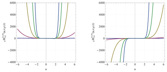
Figure 1. Curves of ${}_C{\mathcal{H}}_{n,1/2}^{(1,2)}(u,0;5;1)$.

The surface plot of ${}_C{\mathcal{H}}_{n,1/2}^{(1,2)}(u,v;5;1)$$(u,v\in \mathbb{R})$ for $n=20$ and $n=21$ are shown in Figure 2.

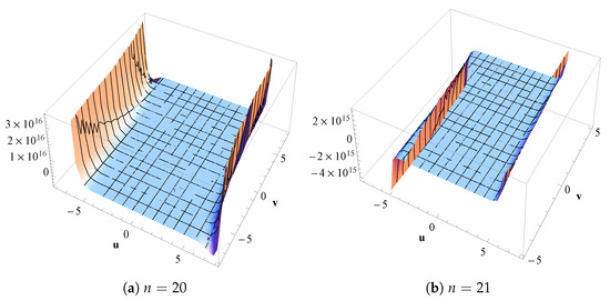
Figure 2. Surface plot of ${}_C{\mathcal{H}}_{20,1/2}^{(1,2)}(u,v;5;1)$ and ${}_C{\mathcal{H}}_{21,1/2}^{(1,2)}(u,v;5;1)$.

Graphs of the qGTATFEP ${}_C{\mathcal{H}}_{n,q}^{(\alpha ,m)}(u,v;\rho ;\lambda )$ for $u=0,-15\le v\le 15$, $n=2$ and for parameters $\alpha =1,\lambda =1,m=2,\rho =5$ and for different values of q$(q=-1/4,-1/8,0,1/8,1/4)$ are given in Figure 3.

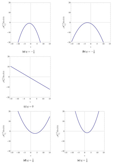
Figure 3. Graphs of qGTATFEP ${}_C{\mathcal{H}}_{n,q}^{(\alpha ,m)}(u,v;\rho ;\lambda )$ for $n=2$ and different values of q.

Further, graphs of the qGTATFEP ${}_C{\mathcal{H}}_{n,q}^{(\alpha ,m)}(u,v;\rho ;\lambda )$ for $u=0,-100\le v\le 100$, $n=3$ and for parameters $\alpha =1,\lambda =1,m=2,\rho =5$ and for different values of q$(q=-1/4,-1/8,0,1/8,1/4)$ are provided in Figure 4.

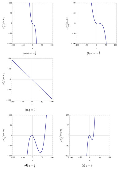
Figure 4. Graphs of qGTATFEP ${}_C{\mathcal{H}}_{n,q}^{(\alpha ,m)}(u,v;\rho ;\lambda )$ for $n=3$ and different values of q.

The numbers of real and complex zeros of ${}_C{\mathcal{H}}_{n,1/2}^{(1,2)}(u,0;5;1)$ along with its approximate values are listed in Table 3.

Table 3. Approximate solutions of ${}_C{\mathcal{H}}_{n,1/2}^{(1,2)}(u,0;5;1)=0$.

n	Number of Real Zeros	Real Zeros	Number of Complex Zeros	Complex Zeros
1	1	$0.75$	0	–
2	2	$-0.3582,1.4831$	0	–
3	3	$-0.5586,0.0639,1.8072$	0	–
4	2	$0.6511,1.8944$	2	$-0.5697-0.4243i$,    $-0.5697+0.4243i$
5	3	$-0.5004,1.0454,1.8690$	2	$-0.4805-0.5538i,-0.4805+0.5538i$
6	4	$-0.8306,0.2763,1.1839,1.8317$	2	$-0.4924-0.7502i,-0.4924+0.7502i$
7	1	$1.8552$	6	$-0.8088-0.3258i,-0.8088+0.3258i,$
				$-0.3704-0.8985i,-0.3704+0.8985i,$
				$0.9958-0.3151i,0.9958+0.3151i$
8	2	$-0.7503,1.9017$	6	$-0.6958-0.4644i,-0.6958+0.4644i,$
				$-0.2647-0.9521i,-0.2647+0.9521i,$
				$1.1319-0.5354i,1.1319+0.5354i$
9	3	$-0.8649,-0.1451,1.9335$	6	$-0.7019-0.5655i,-0.7019+0.5655i,$
				$-0.2056-0.9920i,-0.2056+0.9920i,$
				$1.1943-0.6182i,1.1943+0.6182i$

Figure 5 shows how the zeros of ${}_C{\mathcal{H}}_{20,1/2}^{(1,m)}(u,0;5;1)$ can be located in the complex u-plane as the m grows from 10, 20, 30 and 40.

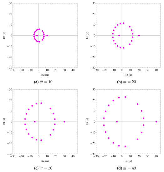
Figure 5. Zeros of ${}_C{\mathcal{H}}_{20,1/2}^{(1,m)}(u,0;5;1)$.

If each approximate real zeros of ${}_C{\mathcal{H}}_{n,1/2}^{(1,2)}(u,0;5;1)$, $(u\in \mathbb{R})$ is piled up according to the value of n for $1\le n\le 20$, it will appear as shown in Figure 6. The values of real zeros for $1\le n\le 9$ are listed in Table 3.

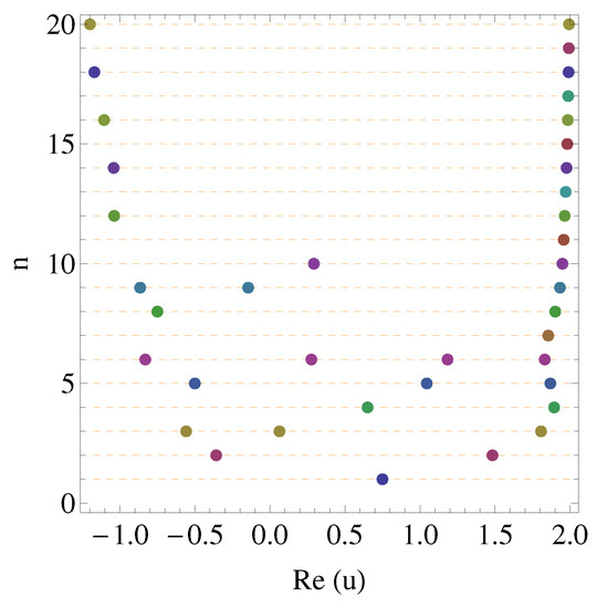
Figure 6. Real zeros of ${}_C{\mathcal{H}}_{n,1/2}^{(1,2)}(u,0;5;1)=0$.

A stack of zeros of ${}_C{\mathcal{H}}_{n,1/2}^{(1,2)}(u,0;5;1)$ for $1\le n\le 20$ which are displayed in the 3-dimensional space are presented in Figure 7.

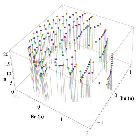
Figure 7. Stacks of zeros of ${}_C{\mathcal{H}}_{n,1/2}^{(1,2)}(u,0;5;1)=0$.

7. Concluding Remarks, Further Observations, and Posing Questions

Recently, due mainly to their importance and diverse applications, a growing number of polynomials and numbers, and their variants and generalizations have been introduced and investigated. In the wake of this trend, by combining the polynomials in Definitions 1 and 5, we introduced the 2-variable q-generalized tangent based Apostol type Frobenius–Euler polynomials ${}_C{\mathcal{H}}_{n,q}^{(\alpha ,m)}(u,v;\rho ;\lambda )$ of order $\alpha$ in the variables u and v. Then we presented a number of properties and formulas for these polynomials such as explicit representations, series representations, summation formulas, addition formula, q-derivative and q-integral formulas. Moreover, using computer-aid programs (e.g., Mathematica, or Matlab), we tried to draw graphs of certain specialized polynomials introduced here. Through those graphs, a number of questions about certain unexpected properties of the polynomials (for example, their zeros) are found to be naturally occurred.

We tried to apply these newly-introduced polynomials to a real world problem (for example, computational fluid dynamics [32,33]). However, we find that it will take a longer period to be familiar with such topics. It remains to be a future investigation.

Observations and Questions

(i)

It may be important to find complex zeros of the following equations

$$\lambda e_q\left(t\right)-\rho =0\mathrm{and}{e}_q\left(mt\right)+1=0$$

(63)

from Definitions 1 and 6 (see also generating functions in Definitions 2, 3, and 5), in particular, in order to determine the $\xi$ and $\eta$ there exactly. When $q=1$, the zeros of two equations in (63) are easily given, respectively, by

$$t=ln\left|\frac{\rho }{\lambda }\right|+i(\vartheta +2k\pi )\mathrm{and}t=i(2k+1)\frac{\pi }{m}(k\in \mathbb{Z}),$$

where $\vartheta$ is an argument of $\frac{\rho }{\lambda }$.

Question 1: Find or approximate the zeros of two equations in (63).

For Question 1, we tried to draw graph of $\lambda e_q\left(t\right)-\rho$ (for $\lambda =1$, $q=\frac{1}{2}$ and $\rho =5$) as follow Figure 8 and Figure 9:

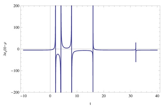Figure 8. Graph of $e_{1/2}\left(t\right)-5$.

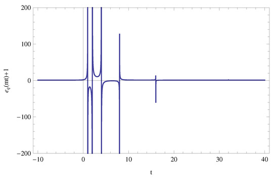Figure 9. Graph of $e_{1/2}\left(2t\right)+1$.

Graph of $e_q\left(mt\right)+1$ (for $m=2$ and $q=\frac{1}{2}$) as follows:

Certain approximate real and complex zeros of

$$e_{1/2}\left(t\right)-5\mathrm{and}{e}_{1/2}\left(2t\right)+1$$

are given, respectively, as

$$1.21057,16.4854,31.929,64.0045;6.18528+1.69686i,6.18528-1.69686i$$

and

$$16.1688;0.812222+1.45191i,0.812222-1.45191i,6.60888+1.45013i,6.60888-1.45013i.$$

(ii)

To approximate zeros of some functions or polynomials, we can use Newton-Raphson’s theorem (see, e.g., [34] (pp. 262–263); for a use of this theorem, one may consult with [11] (Section 6)).

(iii)

It may follow from (47) that ${}_C{\mathcal{H}}_{n,q}^{(\alpha ,m)}(u,v;\rho ;\lambda )$ are polynomials in both u and v of the same degree n.

(iv)

As shown in Figure 5, all zeros of the polynomials ${}_C{\mathcal{H}}_{n,q}^{(\alpha ,m)}(u,b;\rho ;\lambda )$ $(b\in \mathbb{R})$ with the other parameters being real are found to be symmetrically located with respect to the real axis of u (that is, $\Im \left(u\right)=0$). Indeed, if $u_0$ is among its zeros, then, in view of (47), we have

$$0=\overline{{}_C{\mathcal{H}}_{n,q}^{(\alpha ,m)}(u_0,b;\rho ;\lambda )}=\sum _{k=0}^n\frac{{\left[n\right]}_q!}{{\left[k\right]}_q!}{}_C{\mathcal{H}}_{k,q}^{(\alpha ,m)}(\rho ;\lambda ){\mathcal{E}}_{n-k,q}\left(\overline{u_0},b\right),$$

which implies that the complex conjugate $\overline{u_0}$ of $u_0$ is also zero.

One may also recall the reflection principle (see, e.g., [35] (p. 57)).

(v)

In Figure 5, as m becomes larger, the corresponding absolute values (distances from the origin) of zeros of ${}_C{\mathcal{H}}_{20,1/2}^{(1,m)}(u,0;5;1)$ are getting greater (become more distant from the origin).

Question 2: Prove or disprove that this observation is true as $m\uparrow \infty$.

Question 3: Prove or disprove truth of this observation for ${}_C{\mathcal{H}}_{n,q}^{(\alpha ,m)}(u,0;\rho ;\lambda )$ where $m\in {\mathbb{R}}^{+}$ becomes larger and $\left(n\in \mathbb{N},0<q<1,\alpha ,\lambda ,\rho \in \mathbb{R}\right)$.

This can be observed graphically. For several different values of m (−10,000, −1000, 1000, 10,000), graphs of zeros of ${}_C{\mathcal{H}}_{20,1/2}^{(1,2)}(u,0;5;1)$ are demonstrated in Figure 10.

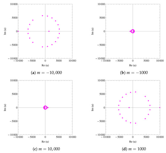Figure 10. Zeros of ${}_C{\mathcal{H}}_{20,1/2}^{(1,2)}(u,0;5;1)$ for different increasing values of m.

(vi)

From Figure 6, the number of real zeros of ${}_C{\mathcal{H}}_{n,1/2}^{(1,2)}(u,0;5;1)$$(1\le n\le 20)$ is observed to range from 1 to 4.

Question 4: Prove or disprove that this observation is true for general $n\in \mathbb{N}$.

Question 5: Prove or disprove truth of this observation for ${}_C{\mathcal{H}}_{n,q}^{(\alpha ,m)}(u,0;\rho ;\lambda )$ where $n\in \mathbb{N}$ varies and $\left(0<q<1,\alpha ,\lambda ,\rho \in \mathbb{R},m\in {\mathbb{R}}^{+}\right)$.

For ${}_C{\mathcal{H}}_{n,1/2}^{(1,2)}(u,0;5;1)$, it is observed experimentally (Mathematica) for n up to 200 that for even values of $n\ge 10$, number of real zeros are 2 and for odd values of $n\ge 10$, number of real zero is 1. For $n<10$, number of zeros are mentioned in Table 3.

(vii)

In each of Definitions 1–5 and Definition 6, the ordinary Taylor (Maclaurin) series expansion is employed, even though each generating function is involved in q-analogues.

Question 6: In the above definitions, it may be really interesting and speculative to see the possible resulting series if the q-Taylor series expansion (see, e.g., [26,28] (Theorem 6.3)) is used, instead of the ordinary Taylor series expansion.

References

- Abdalla, M.; Akel, M.; Choi, J. Certain matrix Riemann–Liouville fractional integrals associated with functions involving generalized Bessel matrix polynomials. Symmetry 2021, 13, 622. [Google Scholar] [CrossRef]
- Bayad, A.; Kim, T. Identities for Apostol-type Frobenius–Euler polynomials resulting from the study of a nonlinear operator. Russ. J. Math. Phys. 2016, 23, 164–171. [Google Scholar] [CrossRef]
- Bildirici, C.; Acikgoz, M.; Araci, S. A note on analogues of tangent polynomials. J. Algebra Number Theor. Acad. 2014, 4, 21–29. [Google Scholar]
- Jain, S.; Nieto, J.J.; Singh, G.; Choi, J. Certain generating relations involving the generalized multi-index Bessel-Maitland function. Math. Prob. Eng. 2020, 2020, 8596736. [Google Scholar] [CrossRef]
- Khammash, G.S.; Agarwal, P.; Choi, J. Extended k-Gamma and k-Beta functions of matrix arguments. Mathematics 2020, 8, 1715. [Google Scholar] [CrossRef]
- Khan, N.U.; Usman, T.; Choi, J. A new class of generalized polynomials involving Laguerre and Euler polynomials. Hacet. J. Math. Stat. 2021, 50, 1–13. [Google Scholar] [CrossRef]
- Kurt, B. A note on the Apostol type q-Frobenius–Euler polynomials and generalizations of the Srivastava-Pinter addition theorems. Filomat 2016, 30, 65–72. [Google Scholar] [CrossRef][Green Version]
- Mahmudov, N.I. On a class of q-Bernoulli and q-Euler polynomials. Adv. Differ. Equ. 2013, 2013, 108. [Google Scholar] [CrossRef]
- Mahmudov, N.I.; Keleshteri, M.E. q-extensions for the Apostol type polynomials. J. Appl. Math. 2014, 2014, 868167. [Google Scholar] [CrossRef]
- Mahmudov, N.I.; Momenzadeh, M. On a class of q-Bernoulli, q-Euler, and q-Genocchi polynomials. Abs. Appl. Anal. 2014, 2014, 696454. [Google Scholar] [CrossRef]
- Nahid, T.; Alam, P.; Choi, J. Truncated-exponential-based Appell-type Changhee polynomials. Symmetry 2020, 12, 1588. [Google Scholar] [CrossRef]
- Ryoo, C.S. A note on the tangent numbers and polynomials. Adv. Stud. Theor. Phys. 2013, 7, 447–454. [Google Scholar] [CrossRef]
- Ryoo, C.S. Generalized tangent numbers and polynomials associated with p-adic integral on Zp. Appl. Math. Sci. 2013, 7, 4929–4934. [Google Scholar] [CrossRef]
- Satoh, J. A construction of q-analogue of Dedekind sums. Nagoya Math. J. 1992, 127, 129–143. Available online: https://projecteuclid.org/euclid.nmj/1118783238 (accessed on 15 March 2021). [CrossRef]
- Simsek, Y. q-analogue of twisted l-series and q-twisted Euler numbers. J. Number Theory 2005, 110, 267–278. [Google Scholar] [CrossRef]
- Simsek, Y. Generating functions for q-Apostol type Frobenius–Euler numbers and polynomials. Axioms 2012, 1, 395–403. [Google Scholar] [CrossRef]
- Usman, T.; Saif, M.; Choi, J. Certain identities associated with (p,q)-binomial coefficients and (p,q)-Stirling Polynomials of the second kind. Symmetry 2020, 12, 1436. [Google Scholar] [CrossRef]
- Yasmin, G.; Muhyi, A. Certain results of 2-variable q-generalized tangent-Apostol type polynomials. J. Math. Comput. Sci. 2020, 22, 238–251. [Google Scholar] [CrossRef]
- Yasmin, G.; Ryoo, C.S.; Islahi, H. A numerical computation of zeros of q-generalized tangent-Appell polynomials. Mathematics 2020, 8, 383. [Google Scholar] [CrossRef]
- Aral, A.; Gupta, V.; Agarwal, R.P. Applications of q-Calculus in Operator Theory; Springer: New York, NY, USA, 2013. [Google Scholar] [CrossRef]
- Dalir, M.; Bashour, M. Applications of fractional calculus. Appl. Math. Sci. 2010, 4, 1021–1032. [Google Scholar]
- Gasper, G.; Rahman, M. Basic Hypergeometric Series, 2nd ed.; Cambridge University Press: Cambridge, UK, 2004. [Google Scholar]
- Andrews, G.E.; Askey, R.; Roy, R. Special Functions; Encyclopedia of Mathematics and Its Applications 71; Cambridge University Press: Cambridge, UK, 1999. [Google Scholar]
- Ernst, T. A newew method for q-calculus. J. Nonlinear Math. Phys. 2003, 10, 487–525. [Google Scholar] [CrossRef]
- Ernst, T. The different tongues of q-calculus. Proc. Est. Acad. Sci. 2008, 57, 81–99. [Google Scholar] [CrossRef]
- Kac, V.G.; Cheung, P. Quantum Calculus; Springer: New York, NY, USA, 2002. [Google Scholar]
- Nalli, P. Sopra un procedimento di calcolo analogo all’integrazione. Palermo Rend. 1923, 47, 337–374. [Google Scholar] [CrossRef]
- Srivastava, H.M.; Choi, J. Zeta and q-Zeta Functions and Associated Series and Integrals; Elsevier Science Publishers: Amsterdam, The Netherlands; London, UK; New York, NY, USA, 2012. [Google Scholar]
- Jackson, F.H. On q-definite integrals. Quart. J. Pure Appl. Math. 1910, 41, 193–203. [Google Scholar]
- Choi, J. Notes on formal manipulations of double series. Commun. Korean Math. Soc. 2003, 18, 781–789. [Google Scholar] [CrossRef]
- Olver, F.W.J.; Lozier, D.W.; Boisvert, R.F.; Clark, C.W. (Eds.) NIST Handbook of Mathematical Functions; NIST and Cambridge University Press: Cambridge, UK; New York, NY, USA; Melbourne, Australia; Madrid, Spain; Cape Town, South Africa; Singapore; São Paulo, Brazil; Delhi, India; Dubai, United Arab Emirates; Tokyo, Japan, 2010. [Google Scholar]
- Bhatti, M.M.; Marin, M.; Zeeshan, A.; Abdelsalam, S.I. Editorial: Recent Trends in Computational Fluid Dynamics. Front. Phys. 2020, 8, 593111. [Google Scholar] [CrossRef]
- Bhatti, M.M.; Marin, M.; Zeeshan, A.; Ellahi, R.; Abdelsalam, S.I. Swimming of motile gyrotactic microorganisms and nanoparticles in blood flow through anisotropically tapered arteries. Front. Phys. 2020, 8, 95. [Google Scholar] [CrossRef]
- Wade, W.R. An Introduction to Analysis, 4th ed.; Pearson Education Inc.: Upper Saddle River, NJ, USA, 2010. [Google Scholar]
- Brown, J.W.; Churchill, R.V. Complex Variables and Applications, 6th ed.; McGraw-Hill International Editions: New York, NY, USA, 1996. [Google Scholar]
Publisher’s Note: MDPI stays neutral with regard to jurisdictional claims in published maps and institutional affiliations. |
© 2021 by the authors. Licensee MDPI, Basel, Switzerland. This article is an open access article distributed under the terms and conditions of the Creative Commons Attribution (CC BY) license (https://creativecommons.org/licenses/by/4.0/).