Abstract
The quick and accurate picking of the first arrival on microseismic signals is one of the critical processing steps of microseismic monitoring. This study proposed a first arrival picking method for application to microseismic data with a low signal-to-noise ratio (SNR). This approach consisted of two steps: feature selection and clustering. First of all, the optimal feature was searched automatically using the ReliefF algorithm according to the weight distribution of the signal features, and without manual design. On that basis, a k-means clustering method was adopted to classify the microseismic data with symmetry (0–1), and the first arrival times were accurately picked. The proposed method was validated using the synthetic data with different noise levels and real microseismic data. The comparative study results indicated that the proposed method had obviously outperformed the classical STA/LTA and the k-means without feature selection. Finally, the microseismic localization of the first arrivals picked using the various methods were compared. The positioning errors were analyzed using box plots with symmetric effect, and those of the proposed method were the smallest, and stable (all of which were less than 0.5 m), which further verified the superiority of this study’s proposed method and its potential in processing complicated microseismic datasets.
1. Introduction
Microseismic monitoring is capable of offering the real-time characteristics of geo-structures by capturing the elastic waves released from rock fractures and realizing the localization of the microseismic events. This method has been widely applied in various fields, such as mining [1,2,3], the construction of tunnels [4,5], slopes [6,7,8], underground cavern explorations [9], and hydraulic fracturing processes [10,11]. The quick and accurate picking of the first arrival for microseismic data is imperative for the data processing of microseismic monitoring [12,13]. However, due to environmental noise and other inevitable interferences, the signal-to-noise ratios (SNR) of the collected microseismic signals tend to be relatively low. Traditional methods cannot meet the high accuracy and efficiency requirements, which make the precise detection of the first arrival time very challenging [14]. It has been found that small errors in the picking time tend to contribute to errors in the localization of the microseismic source, which hinders the assessments of geo-structure damage [15]. The traditional method used to manually determine the first arrival information is labour intensive and time consuming. In addition, it cannot meet the high accuracy and efficiency requirements for the first arrival picking on microseismic signals, particularly under low SNR conditions [16]. Therefore, the development of a fast, accurate, and automatic first arrival picking method from weak microseismic signals under low SNR conditions has received considerable interest in recent years [17].
Based on the fact that the arrivals of primary waves generally produce relatively strong energy waveforms, several methods for the automatic determination of the first arrival time have been proposed. Traditional algorithms for picking microseismic arrival times include short-term average long-term average rations (STA/LTA) [18] and the Akaike information criterion (AIC) [19]. However, both the STA/LTA and AIC picking systems are sensitive to noise, and the picking results tend to be unsatisfactory under low SNR conditions. Time–frequency transform is an effective way to suppress noise and improve the performance of first arrival picking. Furthermore, Kalman filters [20], median filters [21], and other filters [22,23,24] have been successfully utilized to remove the background noise in microseismic data. Wavelet transform [25,26], HHT transform [27], Shearlet transform [28], Radon transform [29], and Intrinsic Time-Scale Decomposition [30] methods have been adopted to preserve effective signal coefficients in transform domains in order to realize the removal of noise from microseismic data. Singular spectrum analysis [31] achieved noise suppression by selecting N major components for the purpose of reconstructing sequences. In recent years, based on dictionary learning [32] or improvements in traditional methods, researchers have successfully conducted studies to attenuate the noise in microseismic data. Nevertheless, the aforementioned de-noising methods tended to damage the useful signals during the noise suppression process. These methods were based on one or several features in the time domain, frequency domain, or other domains in order to remove noise and its components. These features were artificially defined by the amplitudes and frequencies of the signal waveforms. The above-mentioned methods have laid a certain theoretical foundation. However, in practical applications, they have important limitations, and a possibility exists for the decomposition of component waveform distortions.
Recently, machine learning methods have been successfully employed to detect events from time series data for various applications based on the fact that the microseismic data are mainly composed of useful signals and noise under actual conditions. The tasks of the first arrival picking of microseismic data can be treated as classification tasks which categorize the useful signals and noise signals from the raw microseismic data. At the present time, many existing studies have been completed regarding machine learning based on first arrival picking. The Neural Network Method is one of the mostly popular machine learning methods for arrival picking [33,34]. Gentili [35] used a neural network-neural tree (referred to as IUANT2) to quickly and effectively determine P wave and S wave start times. Maity et al. (2014) [36] proposed a new neural network model which utilized multiple derived attributes from data to automatically determine the arrival times of microseismic signals. Kaur et al. (2013) [37] applied back-propagation neural networks (BPNN) to the automatically detect and identify local and regional seismic waves, and then determine p-wave arrival times. However, in real situations, generalized neural network models can only learn the simple features of data sets. The training of very complex models can be very inefficient and may easily lead to over-fitting issues. However, with the advent of the era of big data and the continuous improvements in computer hardware, deep learning has become an extremely powerful technology in the field of artificial intelligence. In recent years, several deep learning-based first arrival picking methods has been proposed. For example, Zhang et al. [38] used an improved WGAN combined with a residual link nested U-Net network to achieve the “end-to-end” output of the microseismic input signals for the purpose of determining the first arrival times. Guo et al. [39] designed a CNN model to classify each sample point of the waveform traces, and then combined a curve fitting method and an unsupervised clustering algorithm in order to determine arrival times. Chen et al. [40] used a two-step method which combined CNN waveform classification and an unsupervised k-means clustering method to select arrival points. However, because the learning processes for the majority of the aforementioned studies were supervised, the performances of the first arrival picking are greatly dependent on the labelled training datasets. Due to their large sizes, labelled data sets are generally unavailable and unsupervised techniques are preferred.
Clustering is a branch of unsupervised methods which are intended to separate the data into groups of similar data points. It can automatically group samples into different clusters without the need for the high-quality labelled training of the datasets. In recent years, the development of clustering-based first arrival picking methods has received considerable interest. Zhu [41] used a fuzzy c-means clustering (FCM) algorithm to pick up the initial time of the signal clusters as the data arrival times according to the similarities between the signals and the noise. Chen [42] applied an unsupervised fuzzy clustering method to determine the arrival times of microseismic data. That type of method utilized three manually selected features (mean, power, and STA/LTA) as the feature vectors for the clustering. Ma [43] adopted local linear embedding (LLE) and an improved particle swarm optimization (PSO) clustering algorithm to select the optimal clustering centres from low-dimensional data via a global search method, and used a k-means clustering algorithm to divide the low-dimensional data into noise and signals. Cano [44] et al. proposed a conditional fuzzy c-means clustering to identify the time intervals of possible wave arrivals, and then used the Akaike Information Criterion (AIC) picker to pick up the arrival time. These progressive techniques have proven that, with properly selected features, clustering methods can be robust to noise and accurately integrate characteristics of different features in order to pick first arrival times. However, this study found that the majority of the aforementioned automatic methods relied on handcrafted features.
In order to tackle the aforementioned issues, a first arrival picking method for microseismic data based on a clustering method with automatic feature selection was introduced in this study. This was a two-step method which combined feature selection with clustering for first arrival time determinations. The feature selection based on the RelifF method was able to reduce the dimensions of the attribute spaces of the microseismic data and automatically identify the optimal features without the need for manually designed features. Once the effective feature vectors had been automatically selected, a clustering method was introduced which could easily determine the first arrivals from the microseismic data. The proposed method was first validated using synthetic data. The comparative study results indicated that the proposed method outperformed the classical STA/LTA and the k-means without feature selection. Furthermore, this study’s experimental test results demonstrated the feasibility of the proposed method using real microseismic data. Finally, the localizations of the microseismic source using the first arrival times obtained using different methods were compared in order to verify the superiority of the proposed method.
2. Experimental Methods
Due to the fact that microseismic data consists of effective signals and noise, the mission of the first arrival picking of the microseismic signals is similar to the classification of the effective signals and noise from the data. However, in the majority of practical situations, the SNRs of time-series microseismic signals are usually low, which makes the identification of effective signals very challenging. In the present study, in order to tackle this issue, it was critical to select informative features which could characterize the effective signals as feature vectors for the clustering processes. Therefore, a first arrival picking method for microseismic data based on clustering with automatic feature selection was introduced, which was defined as a k-means with ReliefF algorithm in this study. It was a two-step method consisting of two cascaded processes: feature selection and clustering for the first arrival time determination. The feature selection step was based on the ReliefF algorithm, which effectively reduced the dimensions of the attribute space of the microseismic data. It was able to automatically determine the optimal feature subset without the requirement of manually designed features. Once the effective feature vectors had been automatically selected, the first arrival times of the effective microseismic signals could be easily classified using the clustering algorithm. The combination of feature selection and first-come, first-served reduced the feature redundancy, and achieved a better performance than the classic k-means clustering method (referred to as k-means without feature selection in this study). The proposed method’s two steps will be elaborated in the following sections.
2.1. ReliefF Algorithm Based the Feature Selection for Microseismic Data
The Relief algorithm [45] was initially limited to the classification of two types of data. However, the latter extended ReliefF algorithm [46] has the ability to solve multi-class problems. The ReliefF algorithm is a feature weighting algorithm which assigns different weights to features according to the correlations of each feature and category. The larger the weight of the feature, the stronger the classification ability of the feature is. The ReliefF algorithm is used to estimate the weights of features according to how well their values can be distinguished among samples which are near to each other.
In this section, the multiple interrelated features for the microseismic data were pre-selected as data preparation for the ReliefF algorithm based on statistical knowledge. The ReliefF algorithm was then used to process the microseismic data and automatically select the feature vectors.
The selections of the feature vectors are vital for clustering-based microseismic first arrival picking. However, because the relevant attributes of the microseismic data are indefinite, manually selected features may not be suitable for microseismic signals with different SNR levels. In this study, the ReliefF algorithm was applied to process the microseismic data and automatically define the feature vectors, rather than using handcrafted features. Initially, eleven possible inter-related dimensional eigenvalues and dimensionless eigenvalues were preselected as features of the microseismic data based on statistical knowledge. These features included the maximum , minimum , mean , range , variance , root mean square , waveform factor , crest factor , pulse factor , margin factor , and power .
After the eleven possible features were calculated, the ReliefF algorithm was adopted to respectively estimate the weights of the various features using distinguishing instances. The ReliefF algorithm randomly selected a sample (), and then searched for its nearest neighbours () from the same class, which were referred to as the nearest hits (), as well as the nearest neighbours (k) from each of the different classes, which were referred to as the nearest misses (). The weight estimations () were updated by the , nearest hit , and nearest miss values of all of the features. Therefore, if the and had different values according to , the would subtract the difference. In contrast, if the and had different values according to , the would add the difference. The weight estimations were defined as follows:
where the contribution for each class of the misses was weighted with the prior probability of that class , which was estimated from the training set. In this study, the represented the prior probabilities for the same classes of , and represented the sum of the probabilities for the miss classes. The process was repeated twenty times. Function was used to calculate the differences between the values of the feature for the two samples and , and was defined as follows:
The specific implementation steps are shown in the flow chart detailed in Figure 1.
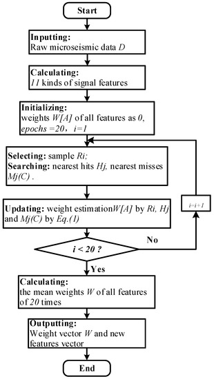
Figure 1.
Flow chart of the feature selection process based on the ReliefF algorithm.
Following the calculations for twenty epochs, the weights of the eleven preselected features were determined, as detailed in the blue histogram in Figure 2. Among those features, the weights of the maximum , range , and root mean square of the signal features were determined to be 0.58, 0.48, and 0.47, respectively, which accounted for the larger weights. At the same time, the weights of the minimum and crest factor were smaller, at 0.15 and 0.20, respectively. This indicated that the maximum , range , and root mean square had the strongest classification abilities among the eleven features selected in this study. Therefore, the first three features with the largest weights selected by the ReliefF algorithm were utilized as the signal features for the k-means clustering in order to determine the first arrival times.
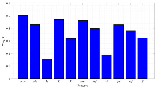
Figure 2.
Weights of the eleven features.
2.2. K-Means Clustering Method Based the Proposed First Arrival Picking
In this study, a k-means clustering method was adopted to process the selected feature vectors and to pick the first arrival times of the microseismic signals. The k-means clustering method is one of the most basic and well-studied unsupervised machine learning algorithms, which was developed by MacQueen in 1967. It is simple in operation, fast in calculation, and sizable to the amounts of datasets [34,37]. The k-means clustering method divides the entire dataset into disjointed clusters. Each data point in the dataset is partitioned to the nearest cluster based on the Euclidean distance matrix. The k-means clustering method is mainly used to distinguish the effective signals and noise from the raw microseismic data . In the current study, was set, which corresponded to the effective signals and noise. For each datum, its attribute vector represents its coordinates in n-dimension space, where the datum is regarded as a point and is the number of features.
The objects were first randomly selected as the centroids of the initial clusters. Then, during each period, after initializing the clusters, the objective functions were calculated. These are generally used to calculate the distances from the members of the cluster to each centroid on all of the clusters as the square error criterion functions. The objective function can be defined as:
where and represent the feature vectors of the datum which has features and the centroid of cluster, respectively. In addition, the Euclidean distances between each point and the initial centroid of each cluster were calculated and defined as follows:
Therefore, by setting the distance between the point and the centroid as , and then assigning each point to the closest group ( or ), the new centroid of each group could be recalculated and defined as follows:
The above-mentioned steps were iterative until the sum of the distances of the member objects to their respective centroids was the smallest over all of the clusters. In the current study, the attribute vector with 0, 1 distribution was obtained by the k-means clustering method. The length was consistent with the signals, and the separation of the signal and noise was successfully realized. Finally, the first change value was extracted as the first arrival time of the signals. The specific implementation steps are shown in the flow chart detailed in Figure 3.
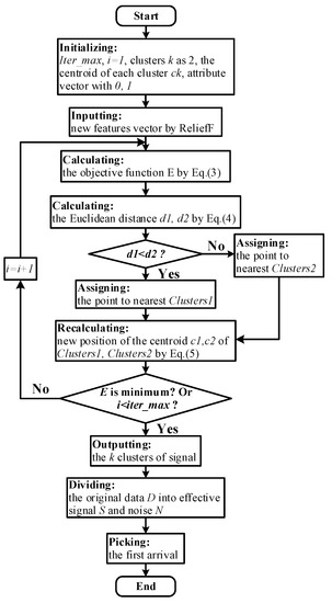
Figure 3.
Flow chart of first arrival picking based on the k-means clustering method.
3. First Arrival Picking Validations Using Synthetic Data
At the initial stage, this study validated the proposed method using a simple and straightforward signal which was one of the microseismic trace signals generated directly from the source. The simulated signal contained three pure Ricker wavelets at 100 ms, 150 ms, and 200 ms, with central frequencies of 70 Hz. The signal had 300 sampling points and the sampling rates were 1 kHz. The amplitudes for the three wavelets were 1,, and , respectively. Subsequently, Gaussian noise was added into the pure signals, and the SNR was −3 dB. Furthermore, the proposed method was utilized to determine the first arrival times of the pure signal and the noisy signal, simultaneously. In Figure 4a, the red perpendicular line represents the times picked by the k-means with ReliefF algorithm, and the picked first arrival time for the pure signal was 88 ms, which could be treated as the real first arrival time according to the results of existing studies [34,36]. Moreover, the first arrival time of the noisy signal was 89 ms, as shown in Figure 4b. The results preliminarily confirmed that the proposed method was feasible for first arrival time determination.
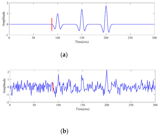
Figure 4.
First arrival picking results of the source signals: (a) pure signal of the sources; (b) noisy signal of the sources with an SNR of −3 dB.
Subsequently, a complex case was explored in order to further validate the proposed method. A two-layered velocity model was simulated, and multiple microseismic trace data were synthetized. The dimensions of the velocity model were 400 m × 600 m, and the localization of the microseismic source was (300, 450), as shown in Figure 5. The velocity of the bottom layer in the model was 3000 m/s, and that of the top layer was 2000 m/s. The blue five-pointed star in Figure 5 indicates the localization of the microseismic source, and the eight black triangles on the top layer denote the eight evenly deployed geophones with intervals of 80 m. This study utilized acoustic waves to simulate the recorded data. In this study, eight traces of cleanmicroseismic signals were obtained. In reality, recorded microseismic signals contain noise. Therefore, the synthetic clean signals were superposed with different types of noise. Finally, three more sets of microseismic signals containing noise, with the SNRs of −2, −4, and −6 dB were formed. The proposed method was then used to pick up the first arrival times for the synthetic data (clean signals and noisy signals). Following the conversation, the first arrivals picked from the clean signals were employed as the reference. Then, for comparison purposes, the classical STA/LTA method was used for all eleven manually selected attributes, as well as the k-means without feature selection. These methods were also utilized to determine the first arrival times for the above-mentioned signals. The long- and short-time windows for the STA/LTA method were 30 ms and 5 ms, respectively.
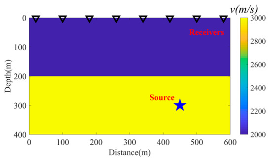
Figure 5.
Two-layered velocity model.
Figure 6 shows the first arrival picking results of the three methods under different noisy conditions. The first arrival times obtained by the proposed method are illustrated by the red perpendicular line in the figure. The black perpendicular line and cyan perpendicular line represent the times picked by the k-means without feature selection, and the classical STA/LTA method, respectively. The first arrival picking results for the clean microseismic signals are depicted in Figure 6a. As can be seen in the figure, all three methods were capable of accurately picking the first arrival times for the eight traces of clean microseismic signals. However, when compared with the results of the proposed method, the first arrival times picked using the k-means without feature selection were slightly earlier. In contrast, the times picked by the classical STA/LTA method were later than those of the proposed method.
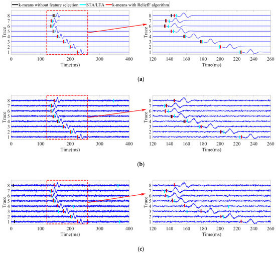
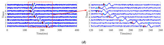
Figure 6.
First arrival picking results of the simulation signals: (a) clean signals; (b) noisy signals with an SNR of −2 dB; (c) noisy signals with an SNR of −4 dB; (d) noisy signals with an SNR of −6 dB.
The first arrival picking results for the signals with SNRs of −2, −4, and −6 dB are shown in Figure 6b–d, respectively. This study further zoomed in on the period range of 120 to 260 ms in the left sub-picture in order to achieve better viewing results. It was observed from the results that when the SNRs were low, the first arrival times received using the classical STA/LTA method displayed obviously large deviations for some traces, such as the eighth traces detailed in Figure 6b; the first, 4th, and eighth traces shown in Figure 6c; and the first, second, fourth, and sixth traces in Figure 6d. Additionally, it was found that the method’s performance continued to worsen as the SNRs decreased. The k-means without feature selection performed better than the STA/LTA method, but still underperformed when compared with the proposed method. For example, when the SNRs were −4 dB and −6 dB, the first arrival times of some of the traces were wrongly detected by the k-means without feature selection method, such as the first and eighth traces in Figure 6c and the third and fifth traces in Figure 6d. The results demonstrate that some handcrafted features were sensitive to noise and had adversely affected the accuracy of the first arrival.
By contrast, the proposed method provided the best performance for all of the SNR conditions in this study. The majority of the first arrival times obtained by the proposed method were found to be in good agreement with the real arrival times, even under the low SNR conditions. Therefore, it was indicated that by using the automatic feature selection operation (ReliefF algorithm), the features which were more robust to noise could be automatically selected in order to achieve accurate first arrival picking performances. The first arrival times picked by the three methods are shown in Table 1. In the table, the value of the “red” mark represents the mis-detected picking of first arrival times.

Table 1.
First arrival picking results of simulation signals with different SNRs.
In the current study, in order to quantitatively measure the superiority of the proposed method, the errors of the deviations between the first arrival times of the clean signals and the noisy signals were calculated. To be specific, this study used the first arrival times of the clean signals as a benchmark, and then used the first arrival times of the noisy signals as the substrate of the benchmark in order to calculate the deviations as follows:
where denotes the errors and denotes the total number of traces, respectively; and denote the first arrival time of the trace in the noisy signals and clean signals, respectively. The errors of the different methods under various noisy conditions are shown as Table 2.
Table 2.
Error of the picking results using the different methods.
It can be seen in the table that when the SNR was −2 dB, the error values of the eight trace signals picked up by the proposed method and the k-means without feature selection were less than 1 ms. In contrast, the error values of the eight trace signals picked by the classical STA/LTA method were 27.25, which was approximately 47 times that of the proposed method. It was observed that, with the increases in the SNR, the errors of first arrival times obtained using the classical STA/LTA method and k-means without feature selection had also increased. However, the error value of the proposed method was only 1.50 ms when the SNR was −6 dB.
It was apparent in this study that the classical STA/LTA method was too sensitive to noise for first arrival picking times, and it had difficulty meeting the situation requirements when the micro-seismic signals had low SNR. In addition, for the k-means without feature selection, it was observed that with all of the eleven dimensional feature vectors, the errors in the arrival times increased when the SNR decreased. This was probably due to irrelevant and redundant features adversely impacting the accuracy of the results. Moreover, the more features computed in a clustering algorithm, the lower the calculation efficiency. Therefore, when compared with the other two clustering methods, the k-means with ReliefF algorithm was more accurate, even under low SNR conditions.
4. Validations Using Real Data and Source Localization
4.1. Validations of the Real Data
In order to further prove the feasibility and accuracy of the first arrival picking of the method proposed in this study, field tests were carried out. The field tests were conducted on a concrete ground surface, as shown in Figure 7a. In the tests, four microseismic sensors were arranged on the ground in a square array, as illustrated in Figure 7b. The side length of the square array was 5 m. Then, by assuming that the coordinates of the No. 1 sensor were (5, 5), the coordinates of the No. 2 sensor were (0, 5), the coordinates of the No. 3 sensor were (5, 0), and the coordinates of the No. 4 sensor were (0, 0), which were referred to as Sensor 1, Sensor 2, Sensor 3, and Sensor 4, respectively. Microseismic sensors were used for the data acquisition in the tests. The sampling frequency range of the microseismic sensors was between 1 and 15 kHz. The microseismic sensors were coupled with the ground using Vaseline. The sampling frequency which was set by the monitoring system was 30 kHz. Three points in the sensor array were selected as the preset source positions, and were referred to as the P1 point (2, 1), P2 point (3, 4), and P3 point (2, 4), respectively. A small hammer was used to strike the ground as a source to generate microseismic signals. The field test diagram and schematic diagram are detailed in Figure 7.
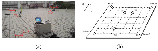
Figure 7.
Field test chart and schematic diagram: (a) field test diagram; (b) schematic diagram.
The method proposed in this study (k-means with ReliefF algorithm) was adopted for the first arrival picking of a set of data of three pre-set source locations (P1, P2, and P3). Next, the results were compared with those of the classical STA/LTA method and k-means without feature selection. The results are shown in Figure 8, Figure 9 and Figure 10, respectively. Similarly, the red perpendicular line, cyan perpendicular line, and black perpendicular line indicate the results of the three methods. It can be seen in the figures that the first arrival times of the microseismic signal data of the four channels were similar due to the close distances between the sensors. Therefore, in order to achieve better observational results, this study further enlarged part of the signal in the red dashed box of the left sub-graph, and the corresponding time length was between 3320 and 3340 ms. It can be seen that the first arrival times obtained using the classical STA/LTA method were later, while the first arrival times of the k-means without feature selection were earlier. Among the 12 traces of data received from the three preset source points, five channels of the first arrival picking results of the STA/LTA method showed obvious large deviations, such as the microseismic signals received by Sensor 1, Sensor 2, and Sensor 3 at position point P1 (2, 1), as well as the microseismic signals received by Sensor 1 and Sensor 2 at point P2 (3, 4). The performance of the k-means without feature selection was better than that of the STA/LTA method, but the first arrival picking times were still inaccurate. One trace of the first arrival picking results was visibly mis-detected, i.e., the microseismic signal received by Sensor 2 at position point P1 (2, 1). In contrast, the proposed k-means with ReliefF algorithm was able to obtain reliable arrival times for the real microseismic data, which were in good agreement with the actual arrival times, thereby confirming the method’s superior performance and feasibility.
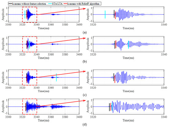
Figure 8.
Microseismic records and the picking of the first arrival times at Point (2, 1): (a) Sensor 1; (b) Sensor 2; (c) Sensor 3; (d) Sensor 4.
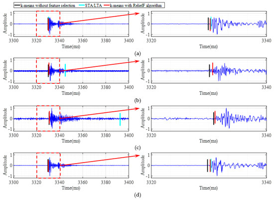
Figure 9.
Microseismic records and the picking of the first arrival times in Point (3, 4): (a) Sensor 1; (b) Sensor 2; (c) Sensor 3; (d) Sensor 4.
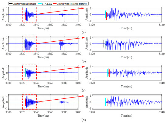
Figure 10.
Microseismic records and the picking of the first arrival times in Point (2, 4): (a) Sensor 1; (b) Sensor 2; (c) Sensor 3; (d) Sensor 4.
The statistics of the first arrival times extracted by the three methods are detailed in Table 3. The value of the “red” mark represents the mis-detected times of the first arrival. The results showed that the classical STA/LTA method had the highest error rate for the first arrival picking times of the real signals. The picking results of the k-means without feature selection were also more sensitive to noise, and the front noise was picked in error as the first arrival of signal. However, the k-means with ReliefF algorithm was able to obtain reliable arrival times using automatic feature selection.
Table 3.
First arrival picking results of real microseismic data at three points.
4.2. Microseismic Localization
In order to verify the accuracy of first arrival picking, this study directly used the first arrival signals extracted by the three methods in Section 4.1, and adopted a genetic algorithm to realize the localization of the microseismic sources. Then, according to the positioning effects, this study made an intuitive comparison in order to verify the feasibility and accuracy of the k-means with ReliefF algorithm proposed in this study. On that basis, repeated experimental tests were used to verify the stability of the proposed method.
A genetic algorithm was used to realize the localization of the microseismic sources. First of all, 50 individuals were randomly selected as the initial population, and the cumulative sum of the arrival time differences for each sensor was taken as the individual fitness function. Then, a roulette wheel selection process was performed on all of the sampling points in order to generate new individuals. At that point, a two-point crossover method was adopted in order to generate individuals, and each individual was mutated by a flipping mutation process. The probabilities of the crossovers and mutations were 0.3 and 0.01, respectively. The termination conditions were met when the fitness function was less than the given error value, or if the number of iterations was maximized. The positioning results were then output [47].
Using the method proposed in this study, the first arrival picking and localization of the microseismic sources were performed in every 20 groups of the repetitive tests for the three source points. The average value of the obtained locating positions was calculated and displayed on the plane coordinate map at the same time as the real source position. Then, the results obtained using the classical STA/LTA method and k-means without feature selection were compared with those achieved using the proposed method, as showed in Figure 11. In the figure, the blue five-pointed star represents the real source position; the red “+” symbol represents the method proposed in this study, namely a k-means with ReliefF algorithm; the bright blue “○” symbol represents the STA/LTA method; and the black “×” symbol represents the k-means without feature selection. It can be seen in the figure that the localization results of the microseismic source of the picking of the first arrival times based on the classical STA/LTA method greatly deviated from the real source position. The source positioning results from the picking of the first arrival times based on the k-means without feature selection were close to the actual source position. However, the distance between the source location of the first arrival picking time based on the proposed method and the actual source position was the smallest.
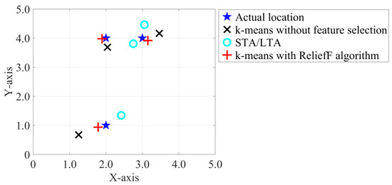
Figure 11.
The localization results of the microseismic sources.
In order to quantitatively analyse the advantages and disadvantages of the three methods, this study calculated the absolute error between the average value of the positioning results and the pre-set source position, as detailed in Table 4. The positioning errors of the classical STA/LTA method for P1 (2, 1), P2 (3, 4), and P3 (2, 4) were 1.02, 0.74, and 0.85, respectively. The positioning errors of the k-means without feature selection for the same source points were 0.67, 0.30, and 0.42, respectively. The positioning errors of the proposed method for the source points were 0.41, 0.17, and 0.22, respectively. The results showed that the proposed k-means with ReliefF algorithm has the smallest rates of error and the best effects in the source positioning results of the first arrival picking. The absolute errors between the pre-set source positions in the tests were less than 0.5 m, and the error relative to the edge length of the sensor array was less than 10%. The feasibility and accuracy of the method proposed in this study were verified in the real microseismic data. Due to the heterogeneity of the materials, the true wave velocities of the microseismic signals in all directions were not completely equal, and the source positioning error was mainly caused by the wave velocity used in the calculation process.
Table 4.
Positioning errors of the three points using the three methods.
During the process of repeated test analyses, boxplotting is an essential tool because it provides a preliminary impression of the underlying distribution shape, which directly affects the evaluations of the first arrival picking time methods [41]. In order to further analyse the stability of the proposed method, this study conducted a boxplot analysis on the positioning errors of every 20 groups of the repetitive tests for the three source points, as shown in Figure 12. More specifically, the symmetry of the error shape was represented by a boxplot at the skewness formed by the 25th percentile (lower end of the box), 50th percentile (interior) and the 75th percentile (upper end). This study used the k-means with ReliefF algorithm to determine the boxplot of the localization errors of the three source points, and compared the result with those of the classical STA/LTA method and the k-means without feature selection, as shown in Figure 12a–c, respectively. In the figure, the red, cyan, and black boxplots represent the error distribution of the locating results of the k-means with ReliefF algorithm, STA/LTA, and k-means without features selection, respectively.
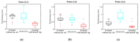
Figure 12.
Boxplot of the positioning errors after 20 repetitions using the three methods: (a) Point (2, 1); (b) Point (3, 4); (c) Point (2, 4).
The obtained statistical dataset showed that abnormal values could be observed in each positioning scheme analysed in this study, which includes the outliers in Figure 12 marked with a red “+” symbol. However, the results of the localization of the microseismic sources based on the proposed method show that the error outliers were less than 1. The dimension height between the maximum and minimum values, and the dimension height between the 25th percentile and the 75th percentile of the boxplot of the method proposed in this study were the minimum, and the 50th percentile was the lowest in the boxplot. The dimension height between the maximum and minimum values of the positioning error boxplots corresponding to the other two methods, and the dimension height between the 25th percentile and the 75th percentile, were much larger than the value of the proposed method. Therefore, the first arrival time picking based on the k-means with ReliefF algorithm for the purpose of the localization had displayed a narrow distribution range of positioning errors, stable positioning results, and small average positioning errors, thereby showing excellent positioning accuracy and stability, which further verified the advantages of the proposed method.
5. Conclusions
In the present study, the focus was placed on the problems related to the rapid and accurate first arrival picking of microseismic signals. A method was proposed which was based on combining clustering with automatic feature selection. In order to evaluate the performance of the proposed method, this study adopted the classical STA/LTA and k-means without feature selection on the same waveform as the references. The main conclusions of this study were the following:
(1) The feature selection based on the ReliefF algorithm has the ability to automatically find the optimal features according to the weight distribution of the signal features, without the need for the manual design of the features. The ReliefF algorithm was used to calculate eleven dimensional eigenvalues and dimensionless eigenvalues twenty times. Among those, the weights of the maximum , range , and root mean square of the signal features were determined to be 0.58, 0.48, and 0.47 respectively, which accounted for the large weights. This indicated that these had the strongest classification abilities among the eleven features. Then, using the three features with the largest weights as the signal features of the k-means clustering for the classification process, the signal feature redundancy was effectively reduced, which easily ensured the separation of the signals and noise.
(2) In the simulation analysis process, this study first directly used a trace of the microseismic signals generated from the source. The k-means with ReliefF algorithm was used to pick up the first arrival point of the pure signal at 88 ms, and at 89 ms for the noisy signal containing −3 dB Gaussian white noise. Those results preliminarily confirmed that the proposed method was feasible for picking the first arrival times. In addition, the proposed method was adopted to pick up the first arrival of the signals with an SNR of −2, −4, and −6 dB. The arrival errors of the eight traces of data using the method proposed in this study were found to be the smallest. For example, when the SNR was −6 dB, the arrival error was only 1.50 ms and tended to be stable with strong robustness. The proposed method was found to be visibly superior to the classical STA/LTA clustering method and the k-means without feature selection.
(3) Experiments were also conducted on real microseismic data in this study. The classical STA/LTA method was observed to have the highest first arrival picking error rate for the real microseismic data. Among the twelve traces of received data, five traces were shown to display obvious large deviations. However, the performance of the k-means without feature selection was better than that of the STA/LTA method, with one trace visibly detected in error. The k-means with ReliefF algorithm proposed in this study was able to obtain reliable arrival times which were in good agreement with the actual arrival times, thereby showing the best performance and feasibility. On that basis, a genetic algorithm was used for the localization. The k-means with ReliefF algorithm picked up the first arrival to realize the localization of the microseismic source, and had the smallest error rate and the best effects, with an absolute error within 0.5 m. In addition, the relative error with the sensor array side length was less than 10%. Furthermore, the results confirmed that the distribution size and height of the positioning error boxplot based on the k-means with ReliefF algorithm were the minimum, and that the positioning errors were small. In addition, the distribution range was narrow, and it showed excellent positioning accuracy and stability, which further verified the superiority of the proposed method.
Therefore, the method combining ReliefF and K-means clustering was used in this paper to pick up the first arrival time of microseismic signals effectively and accurately, which tended to be stable with strong robustness. The results of this study confirmed that the k-means with ReliefF algorithm will potentially be promising for future practical applications in microseismic monitoring projects.
Author Contributions
Y.L., methodology, validation, writing—original draft preparation, and visualization; Z.W., conceptualization, formal analysis, writing—review and editing, supervision, project management, and funding acquisition; J.W., supervision, project management, and funding acquisition; Q.S., supervision, and project management; S.L., conceptualization, methodology, and software; H.W., data curation and project administration; Z.C., formal analysis and investigation. All authors have read and agreed to the published version of the manuscript.
Funding
This research was supported by the National Natural Science Foundation of China (Grant No.: 41877230), Shandong Provincial Key Research and Development Program (SPKR&DP) (Grant No.: 2019GGX101027), and the National Natural Science Foundation of Shandong Province, China (Grant No.:ZR2018MEE052).
Conflicts of Interest
The authors declare no conflict of interest.
References
- Dong, L.J.; Zou, W.; Li, X.B.; Shu, W.W.; Wang, Z.W. Collaborative localization method using analytical and iterative solutions for microseismic/acoustic emission sources in the rockmass structure for underground mining. Eng. Fract. Mech. 2018, 210, 95–112. [Google Scholar] [CrossRef]
- Ge, M. Efficient mine microseismic monitoring. Int. J. Coal Geol. 2005, 64, 44–56. [Google Scholar] [CrossRef]
- Wilkins, A.H.; Strange, A.; Duan, Y.; Luo, X. Identifying microseismic events in a mining scenario using a convolutional neural network. Comput. Geosci. 2020, 137, 104418. [Google Scholar] [CrossRef]
- Feng, G.L.; Feng, X.T.; Chen, B.R.; Xiao, Y.X.; Jiang, Q.; Li, S.J. Temperal-Spatial characteristics of microseismic activity in columnar jointed basalt in tunnelling at baihetan hydropower station. China J. Rock Mech. Eng. 2015, 34, 1967–1975. (In Chinese) [Google Scholar]
- Xu, N.W.; Li, T.B.; Dai, F.; Zhang, R.; Tang, C.A.; Tang, L.X. Microseismic monitoring of strainburst activities in deep tunnels at the jinping ii hydropower station, china. Rock Mech. Rock Eng. 2016, 49, 981–1000. [Google Scholar] [CrossRef]
- Dai, F.; Li, B.; Xu, N.W.; Meng, G.T.; Wu, J.Y.; Fan, Y.L. Microseismic monitoring of the left bank slope at the baihetan hydropower station, china. Rock Mech. Rock Eng. 2017, 50, 225–232. [Google Scholar] [CrossRef]
- Xu, N.W.; Tang, C.A.; Li, L.C.; Zhou, Z.; Yang, J.Y. Microseismic monitoring and stability analysis of the left bank slope in jinping first stage hydropower station in southwestern china. Int. J. Rock Mech. Min. Sci. 2011, 48, 950–963. [Google Scholar] [CrossRef]
- Yfantis, G.; Pytharouli, S.; Lunn, R.J.; Carvajalb, H.E.M. Microseismic monitoring illuminates phases of slope failure in soft soils. Eng. Geol. 2021, 280, 105940. [Google Scholar] [CrossRef]
- Xu, N.W.; Li, T.B.; Dai, F.; Li, B.; Zhu, Y.G.; Yang, D.S. Microseismic monitoring and stability evaluation for the large scale underground caverns at the houziyan hydropower station in southwest china. Eng. Geol. 2015, 188, 48–67. [Google Scholar] [CrossRef]
- Huang, W.; Wang, R.; Li, H.; Chen, Y. Unveiling the signals from extremely noisy microseismic data for high-Resolution hydraulic fracturing monitoring. Sci. Rep. 2017, 7, 11996. [Google Scholar] [CrossRef]
- Maxwell, S.C.; Rutledge, J.; Jones, R.; Fehler, M. Petroleum reservoir characterization using downhole microseismic monitoring. Geophysics 2010, 75, A129–A175. [Google Scholar] [CrossRef]
- Wang, Y.; Shang, X.; Peng, K. Locating Mine Microseismic Events in a 3D Velocity Model through the Gaussian Beam Reverse-Time Migration Technique. Sensors 2020, 20, 2676. [Google Scholar] [CrossRef] [PubMed]
- Li, N.; Wang, E.Y.; Mao-Chen, G.E. Microseismic monitoring technique and its applications at coal mines: Present status and future prospects. J. China Coal Soc. 2017, 42, 83–96. [Google Scholar]
- Li, H.L.; Tuo, X.G.; Wang, R.L.; Courtois, J. A reliable strategy for improving automatic first arrival picking of high noise three component microseismic data. Seismol. Res. Lett. 2019, 90, 1336–1345. [Google Scholar] [CrossRef]
- Zhu, Q.J.; Jiang, F.X.; Wang, C.W.; Liu, Y.; Wang, J.Q.; Yu, Z.X. Automated microseismic event arrival picking and multichannel recognition and location. J. China Coal Soc. 2013, 38, 397–403. (In Chinese) [Google Scholar]
- Li, Y.; Ni, Z.; Tian, Y.Y. Arrival-time picking method based on approximate negentropy for microseismic data. J. Appl. Geophys. 2018, 152, 100–109. [Google Scholar] [CrossRef]
- Qu, S. Automatic microseismic-event detection via supervised machine learning. In Proceedings of the SEG International Exposition and Annual Meeting, Anaheim, CA, USA, 14–19 October 2018; pp. 2287–2291. [Google Scholar]
- Vaezi, Y.; Baan, M. Comparison of the sta/lta and power spectral density methods for microseismic event detection. Geophys. J. Int. 2015, 203, 1896–1908. [Google Scholar] [CrossRef]
- Li, X.B.; Shang, X.Y.; Morales-Esteban, A.; Wang, Z.W. Identifying p phase arrival of weak events: The akaike information criterion picking application based on the empirical mode decomposition. Comput. Geosci. 2017, 100, 57–66. [Google Scholar] [CrossRef]
- Baziw, E.; Nedilko, B.; Weir-Jones, I. Microseismic event detection kalman filter: Derivation of the noise covariance matrix and automated first break determination for accurate source location estimation. Pure Appl. Geophys. 2004, 161, 303–329. [Google Scholar] [CrossRef]
- Zheng, J.; Lu, J.R.; Jiang, T.Q.; Liang, Z. Microseismic event denoising via adaptive directional vector median filters. Acta Geophys. 2017, 65, 47–54. [Google Scholar] [CrossRef]
- Huang, W.L.; Wang, R.Q.; Zu, S.H.; Chen, Y.K. Low-frequency noise attenuation in seismic and microseismic data using mathematical morphological filtering. Geophys. J. Int. 2017, 222, 1296–1318. [Google Scholar] [CrossRef]
- Hu, R.Q.; Wang, Y.C. A first arrival detection method for low snr microseismic signal. Acta Geophys. 2018, 66, 945–957. [Google Scholar] [CrossRef]
- Iqbal, N.; Zerguine, A.; Kaka, S.L.; Al-Shuhail, A. Observation-Driven Method Based on IIR Wiener Filter for Microseismic Data Denoising. Pure. Appl. Geophys. 2018, 175, 2057–2075. [Google Scholar] [CrossRef]
- Kwietniak, A. Detection of the long period long duration (lpld) events in time- and frequency-Domain. Acta Geophys. 2015, 63, 201–213. [Google Scholar] [CrossRef][Green Version]
- Mousavi, S.M.; Langston, C.A.; Horton, S.P. Automatic microseismic denoising and onset detection using the synchrosqueezed continuous wavelet transform. Geophysics 2016, 81, V341–V355. [Google Scholar] [CrossRef]
- Wang, T.; Zhang, M.C.; Yu, Q.H.; Zhang, H.Y. Comparing the applications of EMD and EEMD on time-Frequency analysis of seismic signal. J. Appl. Geophys. 2012, 83, 29–34. [Google Scholar] [CrossRef]
- Cheng, Y.; Li, Y.; Zhang, C. First arrival time picking for microseismic data based on shearlet transform. J. Appl. Geophys. 2017, 14, 262–271. [Google Scholar] [CrossRef]
- Sabbione, J.I.; Sacchi, M.D.; Velis, D.R. Radon transform-Based microseismic event detection and signal-to-Noise ratio enhancement. J. Appl. Geophys. 2015, 113, 51–63. [Google Scholar] [CrossRef]
- Zhang, R.H.; Zhang, L.H. Method for identifying micro-Seismic p-Arrival by time-Frequency analysis using intrinsic time-Scale decomposition. Acta Geophys. 2015, 63, 468–485. [Google Scholar] [CrossRef]
- Jiang, R.C.; Dai, F.; Liu, Y.; Li, A. A novel method for automatic identification of rock fracture signals in microseismic monitoring. Measurement 2021, 175. [Google Scholar]
- Zhang, C.; Baan, M.V.D.; Chen, T. Unsupervised dictionary learning for signal-to-noise ratio enhancement of array data. Seismol. Res. Lett. 2018, 90, 573–580. [Google Scholar] [CrossRef]
- Akram, J.; Ovcharenko, O.; Peter, D. A robust neural network-based approach for microseismic event detection. In Proceedings of the SEG Technical Program Expanded Abstracts, Houston, TX, USA, 24–29 September 2017. [Google Scholar]
- Maity, D.; Salehi, I. Neuro-Evolutionary event detection technique for downhole microseismic surveys. Comput. Geosci. 2016, 86, 23–33. [Google Scholar] [CrossRef]
- Gentili, S.; Michelini, A. Automatic picking of p and s phases using a neural tree. J. Seismol. 2006, 10, 39–63. [Google Scholar] [CrossRef]
- Maity, D.; Aminzadeh, F.; Karrenbach, M. Novel hybrid artificial neural network based autopicking workflow for passive seismic data. Geophys. Prospect. 2014, 62, 834–847. [Google Scholar] [CrossRef]
- Kaur, K.; Wadhwa, M.; Park, E.K. Detection and identification of seismic P-Waves using Artificial Neural Networks. In Proceedings of the International Joint Conference on Neural Networks, IJCNN, Dallas, TX, USA, 4–9 August 2013; pp. 1–6. [Google Scholar]
- Zhang, J.L.; Sheng, G.Q. First arrival picking of microseismic signals based on nested u-net and wasserstein generative adversarial network. J. Pet. Sci. Eng. 2020, 195, 107527. [Google Scholar] [CrossRef]
- Guo, C.; Zhu, T.; Gao, Y.; Wu, S.C.; Sun, J. Aenet: Automatic picking of p-wave first arrivals using deep learning. IEEE Trans. Geosci. Remote Sens. 2020. [Google Scholar] [CrossRef]
- Chen, Y.K.; Zhang, G.Y.; Bai, M.; Zu, S.H.; Guan, Z.; Zhang, M. Automatic waveform classification and arrival picking based on convolutional neural network. Earth Spa. Sci. 2019, 6, 1244–1261. [Google Scholar] [CrossRef]
- Zhu, D.; Li, Y.; Zhang, C. Automatic time picking for microseismic data based on a fuzzy c-means clustering algorithm. IEEE Geosci. Remote Sens. Lett. 2016, 13, 1900–1904. [Google Scholar] [CrossRef]
- Chen, Y.K. Automatic microseismic event picking via unsupervised machine learning. Geophys. J. Int. 2018, 212, 88–102. [Google Scholar] [CrossRef]
- Ma, H.T.; Wang, T.; Li, Y.; Meng, Y.Q. A time picking method for microseismic data based on LLE and improved PSO clustering algorithm. IEEE Geosci. Remote Sens. Lett. 2018, 15, 1677–1681. [Google Scholar] [CrossRef]
- Cano, E.V.; Akram, J.; Peter, D.; Eisner, L. A fuzzy c-Means assisted AIC workflow for arrival picking on downhole microseismic data. In Proceedings of the SEG’s International Exposition and 89th Annual Meeting, San Antonio, TX, USA, 16 September 2019. [Google Scholar]
- Kononenko, I. Estimating attributes: Analysis and extensions of RELIEF. In Proceedings of the European Conference on Machine Learning on Machine Learning, Berlin, Germany, 6–8 April 1994; pp. 171–182. [Google Scholar]
- Reyes, O.; Morell, C.; Ventura, S. Scalable extensions of the ReliefF algorithm for weighting and selecting features on the multi-label learning context. Neurocomputing 2015, 161, 168–182. [Google Scholar] [CrossRef]
- Wu, Y.T. Source locations for microseismic inversed by genetic algorithm. In Proceedings of the Asia Petroleum and Geoscience Conference and Exhibition, APGCE 2017, Kuala Lumpur, Malaysia, 20–21 November 2017; pp. 23–27. [Google Scholar]
Publisher’s Note: MDPI stays neutral with regard to jurisdictional claims in published maps and institutional affiliations. |
© 2021 by the authors. Licensee MDPI, Basel, Switzerland. This article is an open access article distributed under the terms and conditions of the Creative Commons Attribution (CC BY) license (https://creativecommons.org/licenses/by/4.0/).