The Comparative Study for Solving Fractional-Order Fornberg–Whitham Equation via ρ-Laplace Transform

Abstract

In this article, we also introduced two well-known computational techniques for solving the time-fractional Fornberg–Whitham equations. The methods suggested are the modified form of the variational iteration and Adomian decomposition techniques by $\rho$-Laplace. Furthermore, an illustrative scheme is introduced to verify the accuracy of the available methods. The graphical representation of the exact and derived results is presented to show the suggested approaches reliability. The comparative solution analysis via graphs also represented the higher reliability and accuracy of the current techniques.

1. Introduction

With engineering and science development, non-linear evolution models have been analyzed as the problems to define physical phenomena in plasma waves, fluid mechanics, chemical physics, solid-state physics, etc. For the last few years, therefore, a lot of interest has been paid to the result (both numerical and analytical) of these significant models [1,2,3,4]. Different methods are available in the literature for the approximate and exact results of these models. In current years, fractional calculus (FC) applied in many phenomena in applied sciences, fluid mechanics, physics and other biology can be described as very effective using mathematical tools of FC. The fractional derivatives have occurred in many applied sciences equations such as reaction and diffusion processes, system identification, velocity signal analysis, relaxation of damping behaviour fabrics and creeping of polymer composites [5,6,7,8].

The investigation of non-linear wave models and their application is significant in different areas of engineering. Travelling wave notions are between the most attractive results for non-linear fractional-order partial differential equations (NLFPDEs). NLFPDEs are usually identified as mechanical processes and complex physical. Therefore, it is important to get exact results for non-linear time-fractional partial differential equations [9,10,11,12]. Overall, travelling wave results are between the exciting forms of products for NFPDEs. On the other hand, other NLFPDEs, such as the Camassa–Holm or the Kortewegde–Vries equations, have been well-known to have some moving wave solutions. These are non-linear multi-directional dispersive waves in shallow water design problems [13,14,15,16].

The FWE study is of crucial significance in different areas of mathematical physics. The FWEs [15,16] is defined as

$$\begin{array}{c}\hfill D_{\Im }^{\delta }\mu -D_{\phi \phi \Im }\mu +D_{\phi }\mu =\mu D_{\phi \phi \phi }\mu -\mu D_{\phi }\mu +3D_{\phi }\mu D_{\phi \phi }\mu .\end{array}$$

(1)

The quantities performance of wave deformation, a non-linear dispersive wave model, is shown in the investigation. The FWE is presented as a mathematical model for limiting wave heights and wave breaks, allowing peakon results as a numerical model. In 1978, Fornberg and Whitham achieved a measured outcome of the form $\mu (\phi ,\eta )=C{e}^{\left(\frac{-\phi }{2}-\frac{4\Im }{3}\right)}$, where C is constant. The investigation of FWEs has been carried out by several analytical and numerical techniques, such as Adomian decomposition transform method [17], variational iteration technique [18], Lie Symmetry [19], new iterative method [20], differential transformation method [21], homotopy analysis transformation technique [22] and homotopy-perturbation technique [23].

Recently, Abdeljawad and Fahd [24] introduced the Laplace transformation of the fractional-order Caputo derivatives. We suggested a new iterative technique with $\rho$-Laplace transformation to investigate fractional-order ordinary and partial differential equations with fractional-order Caputo derivative. We apply this novel method for solving many fractional-order differential equations such as linear and non-linear diffusion equation, fractional-order Zakharov–Kuznetsov equation and Fokker–Planck equations. We analyzed the impact of $\delta$ and $\rho$ in the process. The Variational iteration method (VIM) was first introduced by He [25,26] and was effectively implemented to the autonomous ordinary differential equation in [27], to non-linear polycrystalline solids [28], and other areas. Similarly, this technique is modified with $\rho$-Laplace transformation, so the modified method is called the $\rho$-Laplace variational iteration method. Many types of differential equations and partial differential equations have solved VITM. For example, this technique is analyzed for solving the time-fractional differential equation (FDEs) in [27]. In [28], this technique is applied to solve non-linear oscillator models. Compared to Adomian’s decomposition process, VITM solves the problem without the need to compute Adomian’s polynomials. This scheme provides a quick result to the equation, whereas the [29] mesh point techniques provide an analytical solution. This method can also be used to get a close approximation of the exact result. G. Adomian, an American mathematician, developed the Adomian decomposition technique. It focuses on finding series-like results and decomposing the non-linear operator into a sequence, with the terms presently computed using Adomian polynomials [30]. This method is modified with $\rho$-Laplace transform, so the modified approach is the $\rho$-Laplace decomposition method. This technique is used for the non-homogeneous FDEs [31,32,33,34,35,36].

This paper has implemented the $\rho$-Laplace variational iteration method and $\rho$-Laplace decomposition method to solve the time-fractional Fornberg–Whitham equations with the Caputo fractional derivative operator. The $\rho$-LDM and $\rho$-LVIM achieve the approximate results in the form of series results.

2. Basic Definitions

In this section, the fractional generalized derivative, the fractional generalized integral, the Mittag-Lefller function the $\rho$-Laplace transform have been discussed.

Definition 1.

The generalized fractional-order integral δ of a continuous function $f:[0,+\infty ]\to R$ is expressed as [24]

$$\left(I^{\delta ,\rho }f\right)\left(\zeta \right)=\frac{1}{\Gamma \left(\delta \right)}{\int }_0^{\zeta }{\left(\frac{{\zeta }^{\rho }-s^{\rho }}{\rho }\right)}^{\delta -1}\frac{f\left(s\right)ds}{s^{1-\rho }},$$

the gamma function denote by Γ, $\rho >0$, $\zeta >0$ and $0<\delta <1$.

Definition 2.

The generalized fractional-order derivative of δ of a continuous function $f:[0,+\infty ]\to R$ is given as [24].

$$\left(D^{\delta ,\rho }f\right)\left(\zeta \right)=\left(I^{1-\delta ,\rho }f\right)\left(\zeta \right)=\frac{1}{\Gamma (1-\delta )}\left(\frac{d}{d\zeta }\right){\int }_0^{\zeta }{\left(\frac{{\zeta }^{\rho }-s^{\rho }}{\rho }\right)}^{-\delta }\frac{f\left(s\right)ds}{s^{1-\rho }}.$$

where define the gamma function Γ, $\rho >0$, $\zeta >0$ and $0<\delta <1$.

Definition 3.

The Caputo fractional-order derivative δ of a continuous function $f:[0,+\infty ]\to R$ is expressed as [24]

$$\left(D^{\delta ,\rho }f\right)\left(\zeta \right)=\frac{1}{\Gamma (1-\delta )}{\int }_0^{\zeta }{\left(\frac{{\zeta }^{\rho }-s^{\rho }}{\rho }\right)}^{-\delta }{\beta }^n\frac{f\left(s\right)ds}{s^{1-\rho }}.$$

where $n=1$, $\rho >0$, $\zeta >0$, $\beta ={\zeta }^{1-\rho }\frac{d}{d\zeta }$ and $0<\delta <1$.

Definition 4.

The ρ-Laplace transformation of a continuous function $f:[0,+\infty ]\to R$ is given as [24]

$$L_{\rho }\left\{f\left(\zeta \right)\right\}={\int }_0^{\infty }{e}^{-s\frac{{\zeta }^{\rho }}{\rho }}f\left(\zeta \right)\frac{d\zeta }{{\zeta }^{1-\rho }}.$$

The Caputo generalized fractional-order ρ-Laplace transform derivative of a continuous function f is defined by [24].

$$\begin{array}{c}\hfill L_{\rho }\left\{D^{\delta ,\rho }f\left(\zeta \right)\right\}=s^{\delta }{L}_{\rho }\left\{f\left(\zeta \right)\right\}-\sum _{k=0}^{n-1}{s}^{\delta -k-1}\left(I^{\delta ,\rho }{\beta }^{n}f\right)\left(0\right)n=1.\end{array}$$

3. The General Methodology of $\mathbf{\rho }$-LDM

The $\rho$-LDM is a combination of the Laplace decomposition method and the $\rho$-Laplace transformation. In this section, we solve the $\rho$-LDM solution of fractional partial differential equation. The main steps of this method are described as follows:

$$\begin{array}{cc}\hfill & D_{\Im }^{\delta ,\rho }\omega (\phi ,\Im )+\overline{\mathcal{L}}(\phi ,\Im )+\mathcal{N}(\phi ,\Im )-\mathcal{H}(\phi ,\Im )=0,0<\delta \le 1,\hfill \end{array}$$

(2)

where $\overline{L}$ and $\mathcal{N}$ are linear and nonlinear functions, $\mathcal{H}$ is the sources function.

The initial condition is

$$\omega (\phi ,0)=f\left(\phi \right),$$

(3)

Apply $\rho$-Laplace transform to Equation (2),

$$\begin{array}{cc}\hfill L_{\rho }\left[D_{\Im }^{\delta ,\rho }\omega (\phi ,\Im )\right]+& L_{\rho }[\overline{\mathcal{L}}(\phi ,\Im )+\mathcal{N}(\phi ,\Im )-\mathcal{H}(\phi ,\Im )]=0.\hfill \end{array}$$

(4)

Applying the $\rho$-Laplace transformation differentiation property, we get

$$\begin{array}{cc}\hfill & L_{\rho }\left[\omega (\phi ,\Im )\right]=\frac{1}{s}\omega (\phi ,0)+\frac{1}{s^{\delta }}{L}_{\rho }\left[\mathcal{H}(\phi ,\Im )\right]-\frac{1}{s^{\delta }}{L}_{\rho }\{\overline{\mathcal{L}}(\phi ,\Im )+\mathcal{N}(\phi ,\Im )\}].\hfill \end{array}$$

(5)

$\rho$-LDM solution of infinite series $\omega (\phi ,\Im )$,

$$\begin{array}{cc}\hfill & \omega (\phi ,\Im )=\sum _{j=0}^{\infty }{\omega }_m(\phi ,\Im ).\hfill \end{array}$$

(6)

The $\mathcal{N}$ is the nonlinear term defined as

$$\mathcal{N}(\phi ,\Im )=\sum _{j=0}^{\infty }{\mathcal{A}}_m.$$

(7)

So the with the help of Adomian polynomial we can define the nonlinear terms

$$\begin{array}{c}\hfill {\mathcal{A}}_m=\frac{1}{j!}{\left[\frac{{\partial }^m}{\partial {\lambda }^m}\left\{\mathcal{N}\left(\sum _{k=0}^{\infty }{\lambda }^k{\omega }_k\right)\right\}\right]}_{\lambda =0}.\end{array}$$

(8)

Putting Equations (6) and (7) into (5), we get

$$\begin{array}{cc}\hfill L_{\rho }\left[\sum _{j=0}^{\infty }{\omega }_m(\phi ,\Im )\right]=& \frac{1}{s}\omega (\phi ,0)+\frac{1}{s^{\delta }}S\left\{\mathcal{H}(\phi ,\Im )\right\}-\frac{1}{s^{\delta }}{L}_{\rho }\left\{\overline{\mathcal{L}}\left(\sum _{j=0}^{\infty }{\omega }_m\right)+\sum _{j=0}^{\infty }{\mathcal{A}}_m\right\}.\hfill \end{array}$$

(9)

Using the inverse $\rho$-Laplace transform with Equation (9),

$$\begin{array}{cc}\hfill & \sum _{j=0}^{\infty }{\omega }_m(\phi ,\Im )=L_{\rho }^{-1}\left[\frac{1}{s}\omega (\phi ,0)+\frac{1}{s^{\delta }}{L}_{\rho }\left\{\mathcal{H}(\phi ,\Im )\right\}-\frac{1}{s^{\delta }}{L}_{\rho }\left\{\overline{\mathcal{L}}\left(\sum _{j=0}^{\infty }{\omega }_m\right)+\sum _{j=0}^{\infty }{\mathcal{A}}_m\right\}\right].\hfill \end{array}$$

(10)

we define the next terms,

$$\begin{array}{cc}\hfill {\omega }_0(\phi ,\Im )=& L_{\rho }^{-1}\left[\frac{1}{s}\omega (\phi ,0)+\frac{1}{s^{\delta }}{L}_{\rho }\left\{\mathcal{H}(\phi ,\Im )\right\}\right],\hfill \end{array}$$

(11)

$$\begin{array}{cc}\hfill & {\omega }_1(\phi ,\Im )=-L_{\rho }^{-1}\left[\frac{1}{s^{\delta }}{L}_{\rho }\{{\overline{\mathcal{L}}}_1\left({\omega }_0\right)+{\mathcal{A}}_0\}\right].\hfill \end{array}$$

For $m\ge 1$, is expressed as

$$\begin{array}{cc}\hfill & {\omega }_{j+1}(\phi ,\Im )=-L_{\rho }^{-1}\left[\frac{1}{s^{\delta }}{L}_{\rho }\{\overline{\mathcal{L}}\left({\omega }_m\right)+{\mathcal{A}}_m\}\right].\hfill \end{array}$$

4. Convergence Analysis

Theorem 1.

[37] (Uniqueness theorem) Equation has a unique solution whenever $0<\epsilon <1$ where $\epsilon =\frac{({\mathrm{h}}_1+{\mathrm{h}}_2+{\mathrm{h}}_3){\Im }^{\delta +1}}{(\delta -1)!}$.

Theorem 2.

[37] (Convergence Theorem) The series solution (11) and (12) of the problem (3) using $\rho$-LTADM and $\rho$-LTVIM converges if $0<\epsilon <1$.

Proof. 

Let $S_{\ell }$ be the mth partial sum, i.e., $S_{\ell }={\sum }_{j=0}^m{\omega }_{\ell }(\phi ,\Im )$. We shall prove that $S_{\ell }$ is a Cauchy sequence in Banach space E. By using a new formulation of Adomian polynomials we get [37]

$$\begin{array}{cc}\hfill & R\left(S_{\ell }\right)={\widehat{A}}_{\ell }+\sum _{j=0}^{m-1}\widehat{A_j}\hfill \\ \hfill & \aleph \left(S_{\ell }\right)=\widehat{A_{\ell }}+\sum _{n=0}^{m-1}\widehat{A_n}\hfill \end{array}$$

$$\begin{array}{cc}\hfill & \left|\right|S_{\ell }-S_{m-1}\left|\right|=\underset{\Im \in I}{max}|S_{\ell }-S_{m-1}|=\underset{\Im \in I}{max}\left|\sum _{j=n+1}^m\widehat{{\omega }_j}(\phi ,\Im )\right|,j=0,1,2\cdots \hfill \\ \hfill & \le \underset{\Im \in I}{max}\left|\begin{array}{cc}& L_{\rho }^{-1}\{\frac{1}{s^{\delta }}{L}_{\rho }\left\{\left[\sum _{j=n+1}^m\mathrm{k}\left[{\omega }_{j-1}(\phi ,\Im )\right]\right]\right\}\\ & +L_{\rho }^{-1}\{\frac{1}{s^{\delta }}{L}_{\rho }\left\{\left[\sum _{j=n+1}^{m}M\left[{\omega }_{j-1}(\phi ,\Im )\right]\right]\right\}\\ & +L_{\rho }^{-1}\{\frac{1}{s^{\delta }}{L}_{\rho }\left\{\left[\sum _{j=n+1}^m\left[A_{j-1}(\phi ,\Im )\right]\right]\right\}\end{array}\right|,\hfill \\ \hfill & \le \underset{\Im \in I}{max}\left|\begin{array}{cc}& L_{\rho }^{-1}\{\frac{1}{s^{\delta }}{L}_{\rho }\left\{\left[\sum _{j=n+1}^m\mathrm{k}\left[{\omega }_j(\phi ,\Im )\right]\right]\right\}\\ & +L_{\rho }^{-1}\{\frac{1}{s^{\delta }}{L}_{\rho }\left\{\left[\sum _{j=n+1}^{m}M\left[{\omega }_j(\phi ,\Im )\right]\right]\right\}\\ & +L_{\rho }^{-1}\{\frac{1}{s^{\delta }}{L}_{\rho }\left\{\left[\sum _{j=n+1}^m\left[A_j(\phi ,\Im )\right]\right]\right\}\end{array}\right|,\hfill \\ \hfill & \le \underset{\Im \in I}{max}\left|\begin{array}{cc}& L_{\rho }^{-1}\{\frac{1}{s^{\delta }}{L}_{\rho }\left\{\left[\sum _{j=n+1}^m\mathrm{k}[S_{m_1-1}-S_{m_2-1}]\right]\right\}\\ & +L_{\rho }^{-1}\{\frac{1}{s^{\delta }}{L}_{\rho }\left\{\left[\sum _{j=n+1}^{m}M[S_{m_1-1}-S_{m_2-1}]\right]\right\}\\ & +L_{\rho }^{-1}\{\frac{1}{s^{\delta }}{L}_{\rho }\left\{\left[\sum _{j=n+1}^m[S_{m_1-1}-S_{m_2-1}]\right]\right\}\end{array}\right|,\hfill \\ \hfill & \le \underset{\Im \in I}{max}\left|\begin{array}{cc}& L_{\rho }^{-1}\{\frac{1}{s^{\delta }}{L}_{\rho }\left\{\left[\mathrm{k}[S_{m_1-1}-S_{m_2-1}]\right]\right\}\\ & +L_{\rho }^{-1}\{\frac{1}{s^{\delta }}{L}_{\rho }\left\{\left[M[S_{m_1-1}-S_{m_2-1}]\right]\right\}\\ & +L_{\rho }^{-1}\{\frac{1}{s^{\delta }}{L}_{\rho }\left\{\left[[S_{m_1-1}-S_{m_2-1}]\right]\right\}\end{array}\right|,\hfill \\ \hfill & \le {\mathrm{k}}_1\underset{\Im \in I}{max}\left|\begin{array}{c}{L}_{\rho }^{-1}\{\frac{1}{s^{\delta }}{L}_{\rho }\left\{[S_{m_1-1}-S_{m_2-1}]\right\}\end{array}\right|,\hfill \\ \hfill & + {\mathrm{k}}_2\underset{\Im \in I}{max}\left|\begin{array}{c}{L}_{\rho }^{-1}\{\frac{1}{s^{\delta }}{L}_{\rho }\left\{[S_{m_1-1}-S_{m_2-1}]\right\}\end{array}\right|,\hfill \\ \hfill & + {\mathrm{k}}_3\underset{\Im \in I}{max}\left|\begin{array}{c}{L}_{\rho }^{-1}\frac{1}{s^{\delta }}{L}_{\rho }\left\{[S_{m_1-1}-S_{m_2-1}]\right\}\end{array}\right|,\hfill \\ \hfill & =\frac{({\mathrm{k}}_1+{\mathrm{k}}_2+{\mathrm{k}}_3){\Im }^{\delta -1}}{(\delta -1)!}\left|\begin{array}{c}\left|\begin{array}{c}{S}_{m_1-1}-S_{m_2-1}\end{array}\right|\end{array}\right|.\hfill \end{array}$$

Letting $m_1=m_2+1$, we get

$$\left|\left|S_{m_2+1}-S_{m_2}\right|\right| \le \epsilon \left|\left|S_{m_2}-S_{m_2-1}\right|\right| \le {\epsilon }^2\left|\left|S_{m_2-1}-S_{m_2-2}\right|\right| \le \cdots \le {\epsilon }^{m_2}\left|\left|S_1-S_0\right|\right|,$$

where $\epsilon =\frac{({\mathrm{k}}_1+{\mathrm{k}}_2+{\mathrm{k}}_3){\Im }^{\delta -1}}{(\delta -1)!}$ similarly, we have from the triangle inequality we get

$$\begin{array}{cc}& \left|\left|S_{m_1-1}-S_{m_2-1}\right|\right| \le \left|\left|S_{m_1+1}-S_{m_2}\right|\right| + \left|\left|S_{m_1+2}-S_{m_2+1}\right|\right| +\cdots + \left|\left|S_{m_1}-S_{m_1-1}\right|\right|,\hfill \\ & \le \left[{\epsilon }^{m_2}+{\epsilon }^{m_2+1}+\cdots +{\epsilon }^{m_1-1}\right] \le \left|\begin{array}{c}\left|\begin{array}{c}{S}_1+S_0\end{array}\right|\end{array}\right|,\hfill \\ & \le {\epsilon }^{m_2}\left(\frac{1-{\epsilon }^{m_1-m_2}}{\epsilon }\right)\left|\begin{array}{c}\left|\begin{array}{c}{\omega }_1\end{array}\right|\end{array}\right|.\hfill \end{array}$$

Since $0<\epsilon <1$ we have $1-{\epsilon }^{m_1-m_2}<1$

$$\left|\begin{array}{c}\left|\begin{array}{c}{S}_{m_1}+S_{m_2}\end{array}\right|\end{array}\right| \le \frac{{\epsilon }^{m_2}}{1-\epsilon }\le \underset{\Im \in I}{max}\left|\begin{array}{c}\left|\begin{array}{c}\omega \end{array}\right|\end{array}\right|.$$

However $\left|\omega \right|<\infty$ so, as $m_2\to \infty$ then $\left|\right|S_{m_1}-S_{m_2}\left|\right|\to 0$, hence $S_{m_1}$ is a Cauchy sequence, the series ${\sum }_{m_1=0}^{\infty }{\omega }_{m_1}$ converges and the proof is complete.  □

Theorem 3.

[37] (Error estimate) The maximum absolute error of the series solution can be given the following formula

$$\underset{\Im \in I}{max}\left|\begin{array}{c}\omega (\phi ,\Im )-\sum _{\ell =1}^{\infty }{\omega }_{\ell }(\phi ,\Im )\end{array}\right|\le \frac{{\epsilon }^{m_2}}{1-\epsilon }\underset{\Im \in I}{max}\left|\begin{array}{c}\left|\begin{array}{c}{\omega }_1\end{array}\right|\end{array}\right|.$$

5. The General Methodology of $\mathbf{\rho }$-Laplace Variational Iteration Method

In this section we show the general methodology of the $\rho$-Laplace variational iteration method solution for fractional partial differential equations.

$$\begin{array}{cc}\hfill & D_{\Im }^{\delta ,\rho }\omega (\phi ,\Im )+\overline{\mathcal{L}}(\phi ,\Im )+\mathcal{N}(\phi ,\Im )-\mathcal{H}(\phi ,\Im )=0,0<\delta \le 1,\hfill \end{array}$$

(12)

with the initial condition

$$\omega (\phi ,0)=f\left(\phi \right),$$

(13)

The using $\rho$-Laplace transformation to Equation (12),

$$\begin{array}{cc}\hfill L_{\rho }\left[D_{\Im }^{\delta ,\rho }\omega (\phi ,\Im )\right]+& L_{\rho }[\overline{\mathcal{L}}(\phi ,\Im )+\mathcal{N}(\phi ,\Im )-\mathcal{H}(\phi ,\Im )]=0.\hfill \end{array}$$

(14)

Applying the differentiation property of $\rho$-Laplace transform, we get

$$\begin{array}{c}\hfill s^{\delta }{L}_{\rho }\left[\omega (\phi ,\Im )\right]-s^{\delta -1}\omega (\phi ,0)=-L_{\rho }\left[\overline{\mathcal{L}}(\phi ,\Im )+\mathcal{N}(\phi ,\Im )-\mathcal{H}(\phi ,\Im )\right].\end{array}$$

(15)

The Lagrange multiplier is used in the iterative method

$$\begin{array}{cc}\hfill L_{\rho }\left[{\omega }_{j+1}(\phi ,\Im )\right]=& L_{\rho }\left[{\omega }_j(\phi ,\Im )\right]+\lambda \left(s\right)\left[s^{\delta }{L}_{\rho }\left[{\omega }_j(\phi ,\Im )\right]-s^{\delta -1}{\omega }_j(\phi ,0)\right.\hfill \\ \hfill & \left.-L_{\rho }\{\overline{\mathcal{L}}(\phi ,\Im )+\mathcal{N}(\phi ,\Im )\}-L_{\rho }\left[\mathcal{H}(\phi ,\Im )\right]\right].\hfill \end{array}$$

(16)

The Lagrange multiplier is

$$\lambda \left(s\right)=-\frac{1}{s^{\delta }},$$

(17)

using inverse $\rho$-Laplace transform $L^{-1}$, Equation (16), we get

$$\begin{array}{c}\hfill {\omega }_{j+1}(\phi ,\Im )={\omega }_j(\phi ,\Im )-L_{\rho }^{-1}\left[\frac{1}{s^{\delta }}\left[-L_{\rho }\{\overline{\mathcal{L}}(\phi ,\Im )+\mathcal{N}(\phi ,\Im )\}\right]-L_{\rho }\left[\mathcal{H}(\phi ,\Im )\right]\right],\end{array}$$

(18)

the initial value can be defined as

$$\begin{array}{cc}\hfill & {\omega }_0(\phi ,\Im )=L_{\rho }^{-1}\left[\frac{1}{s^{\delta }}\left\{s^{\delta -1}\omega (\phi ,0)\right\}\right].\hfill \end{array}$$

(19)

6. Implementation of Techniques

We now proceed to derive an approximate solution to the time-fractional nonlinear FW equations using suggested techniques with generalized Caputo fractional derivative.

6.1. Problem

Consider the time-fractional nonlinear FWE is given as

$$\begin{array}{cc}\hfill D_{\Im }^{\delta ,\rho }\omega -D_{\phi \phi \Im }\omega +D_{\phi }\omega =& \omega D_{\phi \phi \phi }\omega -\omega D_{\phi }\omega +3D_{\phi }\omega D_{\phi \phi }\omega ,0<\delta \le 1,\hfill \end{array}$$

(20)

the initial condition is

$$\omega (\phi ,0)=e^{\left(\frac{\phi }{2}\right)}.$$

(21)

Taking $\rho$-Laplace transform of (20),

$$\begin{array}{cc}\hfill s^{\delta }{L}_{\rho }\left[\omega (\phi ,\Im )\right]-& s^{\delta -1}\omega (\phi ,0)=L_{\rho }\left[D_{\phi \phi \Im }\omega -D_{\phi }\omega +\omega D_{\phi \phi \phi }\omega -\omega D_{\phi }\omega +3D_{\phi }\omega D_{\phi \phi }\omega \right].\hfill \end{array}$$

Applying inverse $\rho$-Laplace transform

$$\begin{array}{cc}\hfill \omega (\phi ,\Im )=& L_{\rho }^{-1}\left[\frac{\omega (\phi ,0)}{s}-\frac{1}{s^{\delta }}{L}_{\rho }\left[D_{\phi \phi \Im }\omega -D_{\phi }\omega +\omega D_{\phi \phi \phi }\omega -\omega D_{\phi }\omega +3D_{\phi }\omega D_{\phi \phi }\omega \right]\right].\hfill \end{array}$$

Using ADM procedure, we get

$${\omega }_0(\phi ,\Im )=L_{\rho }^{-1}\left[\frac{\omega (\phi ,0)}{s}\right]=L_{\rho }^{-1}\left[\frac{e^{\left(\frac{\phi }{2}\right)}}{s}\right],$$

$${\omega }_0(\phi ,t)=e^{\left(\frac{\phi }{2}\right)},$$

(22)

$$\begin{array}{cc}& \sum _{\ell =0}^{\infty }{\omega }_{\ell +1}(\phi ,\Im )=L_{\rho }^{-1}\left[\frac{1}{s^{\delta }}{L}_{\rho }\left[\sum _{\ell =0}^{\infty }{\left(D_{\phi \phi \Im }\omega \right)}_{\ell }-\sum _{\ell =0}^{\infty }{\left(D_{\phi }\omega \right)}_{\ell }+\sum _{\ell =0}^{\infty }{A}_{\ell }-\sum _{\ell =0}^{\infty }{B}_{\ell }+3\sum _{\ell =0}^{\infty }{C}_{\ell }\right]\right],\ell =0,1,2,\cdots \hfill \end{array}$$

$$\begin{array}{cc}\hfill A_0\left(\omega D_{\phi \phi \phi }\omega \right)& ={\omega }_0{D}_{\phi \phi \phi }{\omega }_0,\hfill \\ \hfill A_1\left(\omega D_{\phi \phi \phi }\omega \right)& ={\omega }_0{D}_{\phi \phi \phi }{\omega }_1+{\omega }_1{D}_{\phi \phi \phi }{\omega }_0,\hfill \\ \hfill A_2\left(\omega D_{\phi \phi \phi }\omega \right)& ={\omega }_1{D}_{\phi \phi \phi }{\omega }_2+{\omega }_1{D}_{\phi \phi \phi }{\omega }_1+{\omega }_2{D}_{\phi \phi \phi }{\omega }_0,\hfill \end{array}$$

$$\begin{array}{cc}& B_0\left(\omega D_{\phi }\omega \right)={\omega }_0{D}_{\phi }{\omega }_0,\hfill \\ & B_1\left(\omega D_{\phi }\omega \right)={\omega }_0{D}_{\phi }{\omega }_1+{\omega }_1{D}_{\phi }{\omega }_0,\hfill \\ & B_2\left(\omega D_{\phi }\omega \right)={\omega }_1{D}_{\phi }{\omega }_2+{\omega }_1{D}_{\phi }{\omega }_1+{\omega }_2{D}_{\phi }{\omega }_0,\hfill \end{array}$$

$$\begin{array}{cc}\hfill C_0\left(D_{\phi }\omega D_{\phi \phi }\omega \right)& =D_{\phi }{\omega }_0{D}_{\phi \phi }{\omega }_0,\hfill \\ \hfill C_1\left(D_{\phi }\omega D_{\phi \phi }\omega \right)& =D_{\phi }{\omega }_0{D}_{\phi \phi }{\omega }_1+D_{\phi }{\omega }_1{D}_{\phi \phi }{\omega }_0,\hfill \\ \hfill C_2\left(D_{\phi }\omega D_{\phi \phi }\omega \right)& =D_{\phi }{\omega }_1{D}_{\phi \phi }{\omega }_2+D_{\phi }{\omega }_1{D}_{\phi \phi }{\omega }_1+D_{\phi }{\omega }_2{D}_{\phi \phi }{\omega }_0,\hfill \end{array}$$

for $\ell =1$

$$\begin{array}{cc}\hfill & {\omega }_1(\phi ,\Im )=L_{\rho }^{-1}\left[\frac{1}{s^{\delta }}{L}_{\rho }\left[D_{\phi \phi \Im }{\omega }_0-D_{\phi }{\omega }_0+A_0-B_0+3C_0\right]\right],\hfill \\ & {\omega }_1(\phi ,t)=-\frac{1}{2}{L}_{\rho }^{-1}\left[\frac{e^{\left(\frac{\phi }{2}\right)}}{s^{\delta +1}}\right]=-\frac{1}{2}{e}^{\left(\frac{\phi }{2}\right)}\frac{{\left(\frac{{\Im }^{\rho }}{\rho }\right)}^{\delta }}{\Gamma (\delta +1)}.\hfill \end{array}$$

(23)

for $\ell =2$

$$\begin{array}{cc}\hfill & {\omega }_2(\phi ,\Im )=L_{\rho }^{-1}\left[\frac{1}{s^{\delta }}{L}_{\rho }\left[D_{\phi \phi \Im }{\omega }_1-D_{\phi }{\omega }_1+A_1-B_1+3C_1\right]\right],\hfill \\ & {\omega }_2(\phi ,\Im )=-\frac{1}{8}{e}^{\left(\frac{\phi }{2}\right)}\frac{{\left(\frac{{\Im }^{\rho }}{\rho }\right)}^{2\delta -1}}{\Gamma \left(2\delta \right)}+\frac{1}{4}{e}^{\left(\frac{\phi }{2}\right)}\frac{{\left(\frac{{\Im }^{\rho }}{\rho }\right)}^{2\delta }}{\Gamma (2\delta +1)},\hfill \end{array}$$

(24)

for $\ell =3$

$$\begin{array}{cc}\hfill {\omega }_3(\phi ,\Im )=& L_{\rho }^{-1}\left[\frac{1}{s^{\delta }}{L}_{\rho }\left[D_{\phi \phi \Im }{\omega }_2-D_{\phi }{\omega }_2+A_2-B_2+3C_2\right]\right],\hfill \\ \hfill {\omega }_3(\phi ,\Im )=& -\frac{1}{32}{e}^{\left(\frac{\phi }{2}\right)}\frac{{\left(\frac{{\Im }^{\rho }}{\rho }\right)}^{3\delta -2}}{\Gamma (3\delta -1)}+\frac{1}{8}{e}^{\left(\frac{\phi }{2}\right)}\frac{{\Im }^{3\delta -1}}{\Gamma \left(3\delta \right)}-\frac{1}{8}{e}^{\left(\frac{\phi }{2}\right)}\frac{{\left(\frac{{\Im }^{\rho }}{\rho }\right)}^{3\delta }}{\Gamma (3\delta +1)},\hfill \end{array}$$

(25)

The $\rho$-LDM result of Example 1 is

$$\omega (\phi ,\Im )={\omega }_0(\phi ,\Im )+{\omega }_1(\phi ,\Im )+{\omega }_2(\phi ,\Im )+{\omega }_3(\phi ,\Im )+{\omega }_4(\phi ,\Im )+\cdots ,$$

$$\begin{array}{cc}\hfill \omega (\phi ,\Im )& =e^{\left(\frac{\phi }{2}\right)}-\frac{1}{2}{e}^{\left(\frac{\phi }{2}\right)}\frac{{\left(\frac{{\Im }^{\rho }}{\rho }\right)}^{\delta }}{\Gamma (\delta +1)}-\frac{1}{8}{e}^{\left(\frac{\phi }{2}\right)}\frac{{\left(\frac{{\Im }^{\rho }}{\rho }\right)}^{2\delta -1}}{\Gamma \left(2\delta \right)}+\frac{1}{4}{e}^{\left(\frac{\phi }{2}\right)}\frac{{\left(\frac{{\Im }^{\rho }}{\rho }\right)}^{2\delta }}{\Gamma (2\delta +1)}-\frac{1}{32}{e}^{\left(\frac{\phi }{2}\right)}\frac{{\left(\frac{{\Im }^{\rho }}{\rho }\right)}^{3\delta -2}}{\Gamma (3\delta -1)}\hfill \\ \hfill & +\frac{1}{8}{e}^{\left(\frac{\phi }{2}\right)}\frac{{\Im }^{3\delta -1}}{\Gamma \left(3\delta \right)}-\frac{1}{8}{e}^{\left(\frac{\phi }{2}\right)}\frac{{\left(\frac{{\Im }^{\rho }}{\rho }\right)}^{3\delta }}{\Gamma (3\delta +1)}-\cdots .\hfill \end{array}$$

(26)

The simplify we can write Equation (26), we get

$$\begin{array}{cc}\hfill \omega (\phi ,\Im )=& e^{\left(\frac{\phi }{2}\right)}\left[1-\frac{{\left(\frac{{\Im }^{\rho }}{\rho }\right)}^{\delta }}{2\Gamma (\delta +1)}-\frac{1}{8}\frac{{\left(\frac{{\Im }^{\rho }}{\rho }\right)}^{2\delta -1}}{\Gamma \left(2\delta \right)}+\frac{1}{4}\frac{{\left(\frac{{\Im }^{\rho }}{\rho }\right)}^{2\delta }}{\Gamma (2\delta +1)}-\frac{1}{32}\frac{{\left(\frac{{\Im }^{\rho }}{\rho }\right)}^{3\delta -2}}{\Gamma (3\delta -1)}+\frac{1}{8}\frac{{\left(\frac{{\Im }^{\rho }}{\rho }\right)}^{3\delta -1}}{\Gamma \left(3\delta \right)}-\frac{1}{8}\frac{{\left(\frac{{\Im }^{\rho }}{\rho }\right)}^{3\delta }}{\Gamma (3\delta +1)}+\cdots \right].\hfill \end{array}$$

(27)

The analytical result by $\rho$-LVIM.

The iteration method apply for Equation (20), we get

$$\begin{array}{cc}\hfill {\omega }_{\ell +1}(\phi ,\Im )={\omega }_{\ell }(\phi ,\Im )-& L_{\rho }^{-1}\left[\frac{1}{s^{\delta }}{L}_{\rho }\left\{s^{\delta }{D}_{\Im }{\omega }_{\ell }-D_{\phi \phi \Im }{\omega }_{\ell }+D_{\phi }{\omega }_{\ell }-{\omega }_{\ell }{D}_{\phi \phi \phi }{\omega }_{\ell }+{\omega }_{\ell }{D}_{\phi }{\omega }_{\ell }\right.\right.\left.\left.-3D_{\phi }{\omega }_{\ell }{D}_{\phi \phi }{\omega }_{\ell }\right\}\right],\hfill \end{array}$$

(28)

where

$$\begin{array}{c}\hfill {\omega }_0(\phi ,\Im )=e^{\left(\frac{\phi }{2}\right)}.\end{array}$$

(29)

For $\ell =0,1,2,\cdots$

$$\begin{array}{cc}\hfill {\omega }_1(\phi ,\Im )& ={\omega }_0(\phi ,\Im )-L_{\rho }^{-1}\left[\frac{1}{s^{\delta }}{L}_{\rho }\left\{s^{\delta }{D}_{\Im }{\omega }_0-D_{\phi \phi \Im }{\omega }_0+D_{\phi }{\omega }_0-{\omega }_0{D}_{\phi \phi \phi }{\omega }_0\right.\right.\hfill \\ \hfill & \left.\left.+{\omega }_0{D}_{\phi }{\omega }_0-3D_{\phi }{\omega }_0{D}_{\phi \phi }{\omega }_0\right\}\right],\hfill \\ \hfill {\omega }_1(\phi ,\Im )& =-\frac{1}{2}{e}^{\left(\frac{\phi }{2}\right)}\frac{{\left(\frac{{\Im }^{\rho }}{\rho }\right)}^{\delta }}{\Gamma (\delta +1)},\hfill \end{array}$$

(30)

$$\begin{array}{cc}\hfill {\omega }_2(\phi ,\Im )& ={\omega }_1(\phi ,\Im )-L_{\rho }^{-1}\left[\frac{1}{s^{\delta }}{L}_{\rho }\left\{s^{\delta }{D}_{\Im }{\omega }_1-D_{\phi \phi \Im }{\omega }_1+D_{\phi }{\omega }_1-{\omega }_1{D}_{\phi \phi \phi }{\omega }_1\right.\right.\hfill \\ \hfill & \left.\left.+{\omega }_1{D}_{\phi }{\omega }_1-3D_{\phi }{\omega }_1{D}_{\phi \phi }{\omega }_1\right\}\right],\hfill \\ \hfill {\omega }_2(\phi ,\Im )& =-\frac{1}{8}{e}^{\left(\frac{\phi }{2}\right)}\frac{{\left(\frac{{\Im }^{\rho }}{\rho }\right)}^{2\delta -1}}{\Gamma \left(2\delta \right)}+\frac{1}{4}{e}^{\left(\frac{\phi }{2}\right)}\frac{{\left(\frac{{\Im }^{\rho }}{\rho }\right)}^{2\delta }}{\Gamma (2\delta +1)},\hfill \end{array}$$

(31)

$$\begin{array}{cc}\hfill {\omega }_3(\phi ,\Im )& ={\omega }_2(\phi ,\Im )-L_{\rho }^{-1}\left[\frac{1}{s^{\delta }}{L}_{\rho }\left\{s^{\delta }{D}_{\Im }{\omega }_2-D_{\phi \phi \Im }{\omega }_2+D_{\phi }{\omega }_2-{\omega }_2{D}_{\phi \phi \phi }{\omega }_2\right.\right.\hfill \\ \hfill & \left.\left.+{\omega }_2{D}_{\phi }{\omega }_2-3D_{\phi }{\omega }_2{D}_{\phi \phi }{\omega }_2\right\}\right],\hfill \\ \hfill {\omega }_3(\phi ,\Im )& =-\frac{1}{32}{e}^{\left(\frac{\phi }{2}\right)}\frac{{\left(\frac{{\Im }^{\rho }}{\rho }\right)}^{3\delta -2}}{\Gamma (3\delta -1)}+\frac{1}{8}{e}^{\left(\frac{\phi }{2}\right)}\frac{{\left(\frac{{\Im }^{\rho }}{\rho }\right)}^{3\delta -1}}{\Gamma \left(3\delta \right)}-\frac{1}{8}{e}^{\left(\frac{\phi }{2}\right)}\frac{{\left(\frac{{\Im }^{\rho }}{\rho }\right)}^{3\delta }}{\Gamma (3\delta +1)},\hfill \end{array}$$

(32)

$$\begin{array}{cc}\hfill \omega (\phi ,\Im )=\sum _{m=0}^{\infty }{\omega }_m\left(\phi \right)& =e^{\left(\frac{\phi }{2}\right)}-\frac{1}{2}{e}^{\left(\frac{\phi }{2}\right)}\frac{{\left(\frac{{\Im }^{\rho }}{\rho }\right)}^{\delta }}{\Gamma (\delta +1)}-\frac{1}{8}{e}^{\left(\frac{\phi }{2}\right)}\frac{{\left(\frac{{\Im }^{\rho }}{\rho }\right)}^{2\delta -1}}{\Gamma \left(2\delta \right)}+\frac{1}{4}{e}^{\left(\frac{\phi }{2}\right)}\frac{{\left(\frac{{\Im }^{\rho }}{\rho }\right)}^{2\delta }}{\Gamma (2\delta +1)}\hfill \\ \hfill & -\frac{1}{32}{e}^{\left(\frac{\phi }{2}\right)}\frac{{\left(\frac{{\Im }^{\rho }}{\rho }\right)}^{3\delta -2}}{\Gamma (3\delta -1)}+\frac{1}{8}{e}^{\left(\frac{\phi }{2}\right)}\frac{{\Im }^{3\delta -1}}{\Gamma \left(3\delta \right)}-\frac{1}{8}{e}^{\left(\frac{\phi }{2}\right)}\frac{{\left(\frac{{\Im }^{\rho }}{\rho }\right)}^{3\delta }}{\Gamma (3\delta +1)}-\cdots .\hfill \end{array}$$

(33)

The exact result of Equation (20) at $\delta =1$,

$$\begin{array}{c}\hfill \omega (\phi ,\Im )=e^{\left(\frac{\phi }{2}-\frac{2\Im }{3}\right)}.\end{array}$$

(34)

Figure 1 shows the $\rho$-LDM and $\rho$-LVIM solution of the fractional Fornberg–Whitham defined by generalized fractional-order Caputo derivative in the space coordinate and time $0<\Im \le 0.5$, $\rho =1$ and $\delta =1$. Figure 2, the 3D graph shows approximate and exact solutions graph at $\delta =1$ and $\rho =0.9$; the figure shows that different fractional-order at $\delta$. Similarly, in Figure 3, the 2D graph of exact and approximate solutions plot at $\delta =1$ and $\rho =0.9$ the figure shows that different fractional-order at $\delta$.

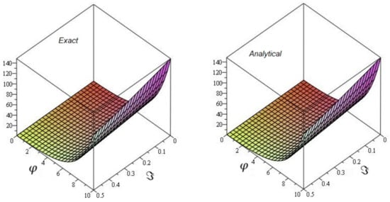
Figure 1. The graph of Exact and analytical solutions of $\delta =1$ and $\rho =1$ of problem 1.

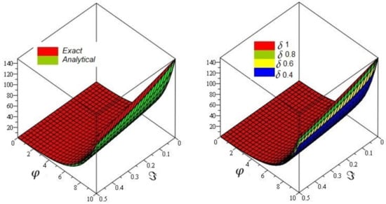
Figure 2. The first 3D graph of Exact and analytical solutions graph at $\delta =1$ and $\rho =0.9$ and second plot of the approximate different fractional-order of $\delta =1$ of problem 1.

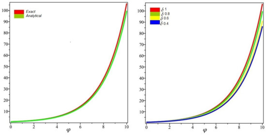
Figure 3. The first 2D graph of Exact and analytical solutions graph at $\delta =1$ and $\rho =0.9$ and second plot of the approximate different fractional-order of $\delta =1$ of problem 1.

6.2. Problem

Consider the time-fractional non-linear FWE given as

$$\begin{array}{cc}\hfill D_{\Im }^{\delta ,\rho }\omega -D_{\phi \phi \Im }\omega +D_{\phi }\omega =& \omega D_{\phi \phi \phi }\omega -\omega D_{\phi }\omega +3D_{\phi }\omega D_{\phi \phi }\omega ,\Im >0,0<\delta \le 1,\hfill \end{array}$$

(35)

with the initial condition

$$\omega (\phi ,0)={cosh}^2\left(\frac{\phi }{4}\right).$$

(36)

Taking $\rho$-Laplace transform of (35),

$$\begin{array}{cc}\hfill s^{\delta }{L}_{\rho }\left[\omega (\phi ,\Im )\right]-& s^{\delta -1}\omega (\phi ,0)=L_{\rho }\left[D_{\phi \phi \Im }\omega -D_{\phi }\omega +\omega D_{\phi \phi \phi }\omega -\omega D_{\phi }\omega +3D_{\phi }\omega D_{\phi \phi }\omega \right].\hfill \end{array}$$

Applying inverse $\rho$-Laplace transform

$$\begin{array}{cc}\hfill \omega (\phi ,\Im )=& L_{\rho }^{-1}\left[\frac{\omega (\phi ,0)}{s}-\frac{1}{s^{\delta }}{L}_{\rho }\left\{D_{\phi \phi \Im }\omega -D_{\phi }\omega +\omega D_{\phi \phi \phi }\omega -\omega D_{\phi }\omega +3D_{\phi }\omega D_{\phi \phi }\omega \right\}\right].\hfill \end{array}$$

Using ADM procedure, we get

$${\omega }_0(\phi ,\Im )=L_{\rho }^{-1}\left[\frac{\omega (\phi ,0)}{s}\right]=L_{\rho }^{-1}\left[\frac{{cosh}^2\left(\frac{\phi }{4}\right)}{s}\right],$$

$${\omega }_0(\phi ,\Im )={cosh}^2\left(\frac{\phi }{4}\right),$$

(37)

$$\begin{array}{cc}& \sum _{\ell =0}^{\infty }{\omega }_{\ell +1}(\phi ,\Im )=L_{\rho }^{-1}\left[\frac{1}{s^{\delta }}{L}_{\rho }\left[\sum _{\ell =0}^{\infty }{\left(D_{\phi \phi \Im }\omega \right)}_{\ell }-\sum _{\ell =0}^{\infty }{\left(D_{\phi }\omega \right)}_{\ell }+\sum _{\ell =0}^{\infty }{A}_{\ell }-\sum _{\ell =0}^{\infty }{B}_{\ell }+3\sum _{\ell =0}^{\infty }{C}_{\ell }\right]\right],\ell =0,1,2,\cdots \hfill \end{array}$$

for $\ell =0$

$$\begin{array}{cc}\hfill {\omega }_1(\phi ,\Im )& =L_{\rho }^{-1}\left[\frac{1}{s^{\delta }}{L}_{\rho }\left[D_{\phi \phi \Im }{\omega }_0-D_{\phi }{\omega }_0+A_0-B_0+3C_0\right]\right],\hfill \\ \hfill {\omega }_1(\phi ,\Im )& =-\frac{11}{32}{L}_{\rho }^{-1}\left[\frac{sinh\left(\frac{x}{2}\right)}{s^{\delta +1}}\right]=-\frac{11}{32}sinh\left(\frac{\phi }{4}\right)\frac{{\left(\frac{{\Im }^{\rho }}{\rho }\right)}^{\delta }}{\Gamma (\delta +1)}.\hfill \end{array}$$

(38)

for $\ell =1$

$$\begin{array}{cc}\hfill {\omega }_2(\phi ,\Im )=& L_{\rho }^{-1}\left[\frac{1}{s^{\delta }}{L}_{\rho }\left[D_{\phi \phi \Im }{\omega }_1-D_{\phi }{\omega }_1+A_1-B_1+3C_1\right]\right],\hfill \\ \hfill {\omega }_2(\phi ,\Im )=& -\frac{11}{28}sinh\left(\frac{\phi }{4}\right)\frac{{\left(\frac{{\Im }^{\rho }}{\rho }\right)}^{\delta }}{\Gamma (\delta +1)}+\frac{121}{1024}cosh\left(\frac{\phi }{4}\right)\frac{{\left(\frac{{\Im }^{\rho }}{\rho }\right)}^{2\delta }}{\Gamma (2\delta +1)},\hfill \end{array}$$

(39)

for $\ell =2$

$$\begin{array}{cc}\hfill {\omega }_3(\phi ,\Im )=& L_{\rho }^{-1}\left[\frac{1}{s^{\delta }}{L}_{\rho }\left[D_{\phi \phi \Im }{\omega }_2-D_{\phi }{\omega }_2+A_2-B_2+3C_2\right]\right],\hfill \\ \hfill {\omega }_3(\phi ,\Im )=& -\frac{11}{512}sinh\left(\frac{\phi }{4}\right)\frac{{\left(\frac{{\Im }^{\rho }}{\rho }\right)}^{\delta }}{\Gamma (\delta +1)}+\frac{121}{2048}cosh\left(\frac{\phi }{4}\right)\frac{{\left(\frac{{\Im }^{\rho }}{\rho }\right)}^{2\delta }}{\Gamma (2\delta +1)}-\frac{1331}{49152}sinh\left(\frac{\phi }{4}\right)\frac{{\left(\frac{{\Im }^{\rho }}{\rho }\right)}^{3\delta }}{\Gamma (3\delta +1)},\hfill \end{array}$$

(40)

The $\rho$-LDM result for problem 2 is

$$\omega (\phi ,\Im )={\omega }_0(\phi ,\Im )+{\omega }_1(\phi ,\Im )+{\omega }_2(\phi ,\Im )+{\omega }_3(\phi ,\Im )+{\omega }_4(\phi ,\Im )+\cdots ,$$

$$\begin{array}{cc}\hfill \omega (\phi ,\Im )& ={cosh}^2\left(\frac{\phi }{4}\right)-\frac{11}{32}sinh\left(\frac{\phi }{4}\right)\frac{{\left(\frac{{\Im }^{\rho }}{\rho }\right)}^{\delta }}{\Gamma (\delta +1)}-\frac{11}{28}sinh\left(\frac{\phi }{4}\right)\frac{{\left(\frac{{\Im }^{\rho }}{\rho }\right)}^{\delta }}{\Gamma (\delta +1)}+\frac{121}{1024}cosh\left(\frac{\phi }{4}\right)\frac{{\left(\frac{{\Im }^{\rho }}{\rho }\right)}^{2\delta }}{\Gamma (2\delta +1)}\hfill \\ \hfill & -\frac{11}{512}sinh\left(\frac{\phi }{4}\right)\frac{{\left(\frac{{\Im }^{\rho }}{\rho }\right)}^{\delta }}{\Gamma (\delta +1)}+\frac{121}{2048}cosh\left(\frac{\phi }{4}\right)\frac{{\left(\frac{{\Im }^{\rho }}{\rho }\right)}^{2\delta }}{\Gamma (2\delta +1)}-\frac{1331}{49152}sinh\left(\frac{\phi }{4}\right)\frac{{\left(\frac{{\Im }^{\rho }}{\rho }\right)}^{3\delta }}{\Gamma (3\delta +1)}\cdots .\hfill \end{array}$$

(41)

The analytical solution by $\rho$-LVIM.

The iteration method is apply by Equation (35), we get

$$\begin{array}{cc}\hfill & {\omega }_{\ell +1}(\phi ,\Im )={\omega }_{\ell }(\phi ,\Im )-L_{\rho }^{-1}\left[\frac{1}{s^{\delta }}{L}_{\rho }\left\{s^{\delta }{D}_{\Im }{\omega }_{\ell }-D_{\phi \phi \Im }{\omega }_{\ell }+D_{\phi }{\omega }_{\ell }-{\omega }_{\ell }{D}_{\phi \phi \phi }{\omega }_{\ell }+{\omega }_{\ell }{D}_{\phi }{\omega }_{\ell }-3D_{\phi }{\omega }_{\ell }{D}_{\phi \phi }{\omega }_{\ell }\right\}\right],\hfill \end{array}$$

(42)

where

$$\begin{array}{c}\hfill {\omega }_0(\phi ,t)={cosh}^2\left(\frac{\phi }{4}\right).\end{array}$$

(43)

For $\ell =0,1,2,\cdots$

$$\begin{array}{cc}\hfill {\omega }_1(\phi ,\Im )& ={\omega }_0(\phi ,\Im )-L_{\rho }^{-1}\left[\frac{1}{s^{\delta }}{L}_{\rho }\left\{s^{\delta }{D}_{\Im }{\omega }_0-D_{\phi \phi \Im }{\omega }_0+D_{\phi }{\omega }_0-{\omega }_0{D}_{\phi \phi \phi }{\omega }_0+{\omega }_0{D}_{\phi }{\omega }_0-3D_{\phi }{\omega }_0{D}_{\phi \phi }{\omega }_0\right\}\right],\hfill \\ \hfill {\omega }_1(\phi ,\Im )& ={cosh}^2\left(\frac{\phi }{4}\right)-\frac{11}{32}sinh\left(\frac{\phi }{4}\right)\frac{{\left(\frac{{\Im }^{\rho }}{\rho }\right)}^{\delta }}{\Gamma (\delta +1)},\hfill \end{array}$$

(44)

$$\begin{array}{cc}\hfill {\omega }_2(\phi ,\Im )& ={\omega }_1(\phi ,\Im )-L_{\rho }^{-1}\left[\frac{1}{s^{\delta }}{L}_{\rho }\left\{s^{\delta }{D}_{\Im }{\omega }_1-D_{\phi \phi \Im }{\omega }_1+D_{\phi }{\omega }_1-{\omega }_1{D}_{\phi \phi \phi }{\omega }_1+{\omega }_1{D}_{\phi }{\omega }_1-3D_{\phi }{\omega }_1{D}_{\phi \phi }{\omega }_1\right\}\right],\hfill \\ \hfill {\omega }_2(\phi ,\Im )& ={cosh}^2\left(\frac{\phi }{4}\right)-\frac{11}{32}sinh\left(\frac{\phi }{4}\right)\frac{{\left(\frac{{\Im }^{\rho }}{\rho }\right)}^{\delta }}{\Gamma (\delta +1)}-\frac{11}{28}sinh\left(\frac{\phi }{4}\right)\frac{{\left(\frac{{\Im }^{\rho }}{\rho }\right)}^{\delta }}{\Gamma (\delta +1)}+\frac{121}{1024}cosh\left(\frac{\phi }{4}\right)\frac{{\left(\frac{{\Im }^{\rho }}{\rho }\right)}^{2\delta }}{\Gamma (2\delta +1)},\hfill \end{array}$$

(45)

$$\begin{array}{cc}\hfill {\omega }_3(\phi ,\Im )={\omega }_2(\phi ,\Im )-& L_{\rho }^{-1}\left[\frac{1}{s^{\delta }}{L}_{\rho }\left\{s^{\delta }{D}_{\Im }{\omega }_2-D_{\phi \phi \Im }{\omega }_2+D_{\phi }{\omega }_2-{\omega }_2{D}_{\phi \phi \phi }{\omega }_2+{\omega }_2{D}_{\phi }{\omega }_2-3D_{\phi }{\omega }_2{D}_{\phi \phi }{\omega }_2\right\}\right],\hfill \\ \hfill {\omega }_3(\phi ,\Im )=& {cosh}^2\left(\frac{\phi }{4}\right)-\frac{11}{32}sinh\left(\frac{\phi }{4}\right)\frac{{\left(\frac{{\Im }^{\rho }}{\rho }\right)}^{\delta }}{\Gamma (\delta +1)}-\frac{11}{28}sinh\left(\frac{\phi }{4}\right)\frac{{\left(\frac{{\Im }^{\rho }}{\rho }\right)}^{\delta }}{\Gamma (\delta +1)}+\frac{121}{1024}cosh\left(\frac{\phi }{4}\right)\frac{{\left(\frac{{\Im }^{\rho }}{\rho }\right)}^{2\delta }}{\Gamma (2\delta +1)},\hfill \\ \hfill & -\frac{11}{512}sinh\left(\frac{\phi }{4}\right)\frac{{\left(\frac{{\Im }^{\rho }}{\rho }\right)}^{\delta }}{\Gamma (\delta +1)}+\frac{121}{2048}cosh\left(\frac{\phi }{4}\right)\frac{{\left(\frac{{\Im }^{\rho }}{\rho }\right)}^{2\delta }}{\Gamma (2\delta +1)}-\frac{1331}{49152}sinh\left(\frac{\phi }{4}\right)\frac{{\left(\frac{{\Im }^{\rho }}{\rho }\right)}^{3\delta }}{\Gamma (3\delta +1)},\hfill \end{array}$$

(46)

$$\begin{array}{cc}\hfill \omega (\phi ,\Im )=& \sum _{m=0}^{\infty }{\omega }_m\left(\phi \right)={cosh}^2\left(\frac{\phi }{4}\right)-\frac{11}{32}sinh\left(\frac{\phi }{4}\right)\frac{{\left(\frac{{\Im }^{\rho }}{\rho }\right)}^{\delta }}{\Gamma (\delta +1)}-\frac{11}{28}sinh\left(\frac{\phi }{4}\right)\frac{{\left(\frac{{\Im }^{\rho }}{\rho }\right)}^{\delta }}{\Gamma (\delta +1)}+\frac{121}{1024}cosh\left(\frac{\phi }{4}\right)\frac{{\left(\frac{{\Im }^{\rho }}{\rho }\right)}^{2\delta }}{\Gamma (2\delta +1)},\hfill \\ \hfill & -\frac{11}{512}sinh\left(\frac{\phi }{4}\right)\frac{{\left(\frac{{\Im }^{\rho }}{\rho }\right)}^{\delta }}{\Gamma (\delta +1)}+\frac{121}{2048}cosh\left(\frac{\phi }{4}\right)\frac{{\left(\frac{{\Im }^{\rho }}{\rho }\right)}^{2\delta }}{\Gamma (2\delta +1)}-\frac{1331}{49152}sinh\left(\frac{\phi }{4}\right)\frac{{\left(\frac{{\Im }^{\rho }}{\rho }\right)}^{3\delta }}{\Gamma (3\delta +1)}-\cdots .\hfill \end{array}$$

(47)

The exact result of Equation (35) at $\delta =1$,

$$\begin{array}{c}\hfill \omega (\phi ,\Im )={cosh}^2\left(\frac{\phi }{4}-\frac{11\Im }{24}\right).\end{array}$$

(48)

Figure 4 shows the $\rho$-LDM and $\rho$-LVIM solution of the fractional Fornberg–Whitham defined by generalized Caputo fractional-order derivative in the space coordinate and time $0<\Im \le 0.5$, $\rho =1$ and $\delta =1$. Figure 5, the 3D graph shows exact and approximate solutions plot at $\delta =1$ and $\rho =0.9$; the figure shows that different fractional-order at $\delta$. Similarly, in Figure 6, the 2D graph of exact and approximate solutions plot at $\delta =1$ and $\rho =0.9$ the figure shows that different fractional-order at $\delta$.

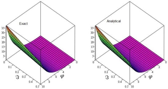
Figure 4. The graph of Exact and approximate solutions of $\delta =1$ and $\rho =1$ of Example 2.

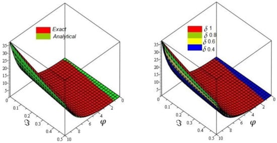
Figure 5. The first 3D graph of Exact and approximate solutions plot at $\delta =1$ and $\rho =0.9$ and second plot of the approximate different fractional-order of $\delta =1$ of Example 2.

Figure 6. The first 2D graph of Exact and approximate solutions plot at $\delta =1$ and $\rho =0.9$ and second plot of the approximate different fractional-order of $\delta =1$ of Example 2.

7. Conclusions

In this article, different semi-analytical techniques are implemented to solve time-fractional Fornberg–Whitham equation. The approximate solution of the equations is evaluated to confirm the validity and reliability of the proposed methods. Graphs of the solutions are plotted to display the closed relation between the obtained and exact results. In addition, the suggested techniques provide easily computable components for the series-form tests. It is investigated that the results achieved in the series form have a higher convergence rate towards the exact results. The proposed methods have a small number of calculations to achieve the approximate solution. In conclusion, it is found that the proposed technique is a sophisticated method for solving other NLFPDEs. In the future, the analytical result of non-linear fractional-order boundary values problems achieved using this technique is in the form of uniform convergence series.

References

- Qureshi, S.; Yusuf, A.; Shaikh, A.A.; Inc, M.; Baleanu, D. Fractional modeling of blood ethanol concentration system with real data application. Chaos Interdiscip. J. Nonlinear Sci. 2019, 29, 013143. [Google Scholar] [CrossRef]
- Yusuf, A.; Qureshi, S.; Inc, M.; Aliyu, A.I.; Baleanu, D.; Shaikh, A.A. Two-strain epidemic model involving fractional derivative with Mittag-Leffler kernel. Chaos Interdiscip. J. Nonlinear Sci. 2018, 28, 123121. [Google Scholar] [CrossRef] [PubMed]
- Kilic, B.; Inc, M. The first integral method for the time fractional Kaup-Boussinesq system with time dependent coefficient. Appl. Math. Comput. 2015, 254, 70–74. [Google Scholar] [CrossRef]
- Inc, M.; Akgul, A.; Kilicman, A. Numerical solutions of the second-order one-dimensional telegraph equation based on reproducing kernel Hilbert space method. Abstr. Appl. Anal. 2013, 2013, 768963. [Google Scholar] [CrossRef]
- Hilfer, R. Applications of Fractional Calculus in Physics; World Scientific: Singapore, 2000; Volume 35, pp. 87–130. [Google Scholar]
- Cesarano, C.; Pierpaolo, N.; Paolo, E.R. Pseudo-Lucas Functions of Fractional Degree and Applications. Axioms 2021, 10, 51. [Google Scholar] [CrossRef]
- Sabatier, J.A.T.M.J.; Agrawal, O.P.; Machado, J.T. Advances in Fractional Calculus; Springer: Dordrecht, The Netherlands, 2007; Volume 4. [Google Scholar]
- Al-luhaibi, M.S. An analytical treatment to fractional Fornberg-Whitham equation. Math. Sci. 2017, 11, 1–6. [Google Scholar] [CrossRef]
- Agarwal, P.; Ahs, S.; Akbare, M.; Nawaz, R.; Cesarano, C. A Reliable Algorithm for solution of Higher Dimensional Nonlinear (1+1) and (2+1) Dimensional Volterra-Fredholm Integral Equations. Dolomites Res. Notes Approx. 2021, 14, 18–25. [Google Scholar]
- Zakarya, M.; Altanji, M.; AlNemer, G.; Abd El-Hamid, H.A.; Cesarano, C.; Rezk, H.M. Fractional Reverse Coposn’s Inequalities via Conformable Calculus on Time Scales. Symmetry 2021, 13, 542. [Google Scholar] [CrossRef]
- Ahmad, I.; Ahmad, H.; Thounthong, P.; Chu, Y.-M.; Cesarano, C. Solution of Multi-Term Time-Fractional PDE Models Arising in Mathematical Biology and Physics by Local Meshless Method. Symmetry 2020, 12, 1195. [Google Scholar] [CrossRef]
- Bazighifan, O.; Cesarano, C. A Philos-type oscillation criteria for fourth-order neutral differential equations. Symmetry 2020, 12, 379. [Google Scholar] [CrossRef]
- Camacho, J.C.; Rosa, M.; Garias, M.L.; Bruzon, M.S. Classical symmetries, travelling wave solutions and conservation laws of a generalized Fornberg-Whitham equation. J. Comput. Appl. Math. 2017, 318, 149–155. [Google Scholar] [CrossRef]
- Bruzon, M.S.; Marquez, A.P.; Garrido, T.M.; Recio, E.; de la Rosa, R. Conservation laws for a generalized seventh order KdV equation. J. Comput. Appl. Math. 2019, 354, 682–688. [Google Scholar] [CrossRef]
- Whitham, G.B. Variational methods and applications to water waves. Proc. R. Soc. Lond. Ser. A Math. Phys. Sci. 1967, 299, 6–25. [Google Scholar]
- Fornberg, B.; Whitham, G.B. A numerical and theoretical study of certain nonlinear wave phenomena. Philos. Trans. R. Soc. Lond. Ser. A Math. Phys. Sci. 1978, 289, 373–404. [Google Scholar]
- Kumar, D.; Singh, J.; Baleanu, D. A new analysis of the Fornberg-Whitham equation pertaining to a fractional derivative with Mittag-Leffler-type kernel. Eur. Phys. J. Plus 2018, 133, 1–10. [Google Scholar] [CrossRef]
- Lu, J. An analytical approach to the Fornberg-Whitham type equations by using the variational iteration method. Comput. Math. Appl. 2011, 61, 2010–2013. [Google Scholar] [CrossRef][Green Version]
- Hashemi, M.S.; Haji-Badali, A.; Vafadar, P. Group invariant solutions and conservation laws of the Fornberg-Whitham equation. Z. Naturforschung A 2014, 69, 489–496. [Google Scholar] [CrossRef]
- Ramadan, M.A.; Al-luhaibi, M.S. New iterative method for solving the fornberg-whitham equation and comparison with homotopy perturbation transform method. J. Adv. Math. Comput. Sci. 2014, 4, 1213–1227. [Google Scholar] [CrossRef]
- Merdan, M.; Gokdogan, A.; Yildirim, A.; Mohyud-Din, S.T. Numerical simulation of fractional Fornberg-Whitham equation by differential transformation method. Abstr. Appl. Anal. 2012, 2012, 965367. [Google Scholar] [CrossRef]
- Wang, K.; Liu, S. Application of new iterative transform method and modified fractional homotopy analysis transform method for fractional Fornberg-Whitham equation. J. Nonlinear Sci. Appl. 2016, 9, 2419–2433. [Google Scholar] [CrossRef]
- Abidi, F.; Omrani, K. Numerical solutions for the nonlinear Fornberg-Whitham equation by He’s methods. Int. J. Mod. Phys. B 2011, 25, 4721–4732. [Google Scholar] [CrossRef]
- Jarad, F.; Abdeljawad, T. A modifi ed Laplace transform for certain generalized fractional operators. Results Nonlinear Anal. 2018, 1, 88–98. [Google Scholar]
- He, J.H. Approximate solution of nonlinear differential equations with convolution product nonlinearities. Comput. Methods Appl. Mech. Eng. 1998, 167, 69–73. [Google Scholar] [CrossRef]
- He, J.H. Variational iteration method for autonomous ordinary differential systems. Appl. Math. Comput. 2000, 114, 115–123. [Google Scholar] [CrossRef]
- Wu, G.C.; Baleanu, D. Variational iteration method for fractional calculus-a universal approach by Laplace transform. Adv. Differ. Equ. 2013, 2013, 18. [Google Scholar] [CrossRef]
- Anjum, N.; He, J.H. Laplace transform: Making the variational iteration method easier. Appl. Math. Lett. 2019, 92, 134–138. [Google Scholar] [CrossRef]
- Dehghan, M. Finite difference procedures for solving a problem arising in modeling and design of certain optoelectronic devices. Math. Comput. Simul. 2006, 71, 16–30. [Google Scholar] [CrossRef]
- Adomian, G. Solving Frontier Problems of Physics: The Decomposition Method; Kluwer Academic Publishers: Boston, MA, USA, 1994. [Google Scholar]
- Khalouta, A.; Kadem, A. A New Method to Solve Fractional Differential Equations: Inverse Fractional Laplace Transform Method. Appl. Appl. Math. 2019, 14, 926–941. [Google Scholar]
- Bokhari, A.; Baleanu, D.; Belgacem, R. Application of Laplace transform to Atangana-Baleanu derivatives. J. Math. Comput. Sci. 2019, 20, 101–107. [Google Scholar] [CrossRef]
- Belgacem, R.; Baleanu, D.; Bokhari, A. Laplace Transform and Applications to Caputo-Fractional Differential Equations. Int. J. Anal. Appl. 2019, 17, 917–927. [Google Scholar]
- Machado, J.; Baleanu, D.; Chen, W.; Sabatier, J. New trends in fractional dynamics. J. Vib. Control 2014, 20, 963. [Google Scholar] [CrossRef]
- Baleanu, D.; Guvenc, Z.; Machado, J. New Trends in Nanotechnology and Fractional Calculus Applications; Springer: Dordrecht, The Netherlands, 2010. [Google Scholar]
- Maitama, S.; Zhao, W. New integral transform: Laplace transform a generalization of Sumudu and Laplace transform for solving differential equations. arXiv 2019, arXiv:1904.11370. [Google Scholar]
- El-Kalla, I.L. Convergence of the Adomian method applied to a class of nonlinear integral equations. Appl. Math. Lett. 2008, 21, 372–376. [Google Scholar] [CrossRef]
Publisher’s Note: MDPI stays neutral with regard to jurisdictional claims in published maps and institutional affiliations. |
© 2021 by the authors. Licensee MDPI, Basel, Switzerland. This article is an open access article distributed under the terms and conditions of the Creative Commons Attribution (CC BY) license (https://creativecommons.org/licenses/by/4.0/).