Article

New Method for Generating New Families of Distributions

by
Lamya A. Baharith
1,* and
Wedad H. Aljuhani
1,2
1
Department of Statistics, Faculty of Science, King Abdulaziz University, Jeddah 21589, Saudi Arabia
2
Department of Statistics, Faculty of Science, University of Tabuk, Tabuk 71491, Saudi Arabia
*
Author to whom correspondence should be addressed.
Symmetry 2021, 13(4), 726; https://doi.org/10.3390/sym13040726
Submission received: 6 March 2021 / Revised: 6 April 2021 / Accepted: 17 April 2021 / Published: 20 April 2021
(This article belongs to the Special Issue Recent Advances in Number Theory and Their Applications)

Abstract

:
This article presents a new method for generating distributions. This method combines two techniques—the transformed—transformer and alpha power transformation approaches—allowing for tremendous flexibility in the resulting distributions. The new approach is applied to introduce the alpha power Weibull—exponential distribution. The density of this distribution can take asymmetric and near-symmetric shapes. Various asymmetric shapes, such as decreasing, increasing, L-shaped, near-symmetrical, and right-skewed shapes, are observed for the related failure rate function, making it more tractable for many modeling applications. Some significant mathematical features of the suggested distribution are determined. Estimates of the unknown parameters of the proposed distribution are obtained using the maximum likelihood method. Furthermore, some numerical studies were carried out, in order to evaluate the estimation performance. Three practical datasets are considered to analyze the usefulness and flexibility of the introduced distribution. The proposed alpha power Weibull–exponential distribution can outperform other well-known distributions, showing its great adaptability in the context of real data analysis.

1. Introduction

Several statistical distributions have been extensively applied to describe and predict existing phenomena in several disciplines, such as economics, engineering, finance, insurance, demography, biology, and environmental and medical sciences. However, in many of these areas, the data usually demonstrate complicated behavior and varied shapes, associated with various degrees of skewness and kurtosis. Thus, many of the existing standard distributions have some limitations when fitting these data, such that applying these classical distributions may not provide an acceptable fit. Therefore, many researchers have attempted to extend these existing classical distributions, in order to obtain greater flexibility in modeling data from different fields of study. Some examples of these modified distributions in the literature include the exponentiated Weibull distribution [1], the exponentiated exponential [2], and the exponentiated Gumbel distribution [3], which are modifications of the well-known Weibull, exponential, and Gumbel distributions, respectively. Extensions of the existing standard models are usually obtained by developing techniques to generate new families of distributions; that is, new generators for families of distributions are defined, in order to improve the goodness-of-fit of the distributions.
Various methods for generating new families of distributions have been studied recently. These include the beta-generating (beta-G) family [4], as well as the Kumaraswamy-generating (Kw-G) family [5]. The beta-G and Kw-G families were developed using distributions defined on the support [0, 1] as generators. The auhtors of [6] developed a general method, called the transformed–transformer (TX) family of distributions, which enable the use of any continuous distribution as the generator. This family can be described as follows:
If r(t) and R(t) are the probability density function (PDF) and cumulative distribution function (CDF) of a random variable (RV) T, respectively, where T [ a , b ] for a < b , then the CDF and PDF of the TX family are expressed, respectively, as
F ( x ) = a W ( G ( x ) ) r ( t ) d t ,
f ( x ) = d d x W ( G ( x ) ) ) r W ( G ( x ) ) ,
where W(G(x)) is a function of the CDF G(x) of any RV X that meets the conditions described in [6].
Many new distributions have been defined and studied on the basis of the TX technique, using different forms of W(G(x)). For example, the study in [7] used W ( G ( x ) ) = log [ G ( x ) / ( 1 G ( x ) ) ] to introduce the Gumbel–Weibull distribution, the study in [8] used W ( G ( x ) ) = log ( 1 G α ( x ) ) to introduce the exponentiated Weibull–exponential distribution, and the studies in [9,10] used W ( G ( x ) ) = log [ 1 G ( x ) ] to introduce the Weibull–Pareto and gamma–normal distributions, respectively.
A new innovative technique, named alpha power transformation (APT), has recently been developed [11]. The APT can be considered a useful method to incorporate skewness into any distribution. The CDF and PDF of an APT family can be expressed as
F A P T ( x ) = α F ( x ) 1 α 1 if   α > 0 ,   α 1 F ( x ) if   α = 1 ,
f A P T ( x ) = log α α 1 f ( x ) α F ( x ) if   α > 0 ,   α 1 f ( x ) if   α = 1 ,
where F ( x ) and f ( x ) represent the CDF and PDF of any continuous distribution, respectively.
Various studies have used this technique to introduce new distributions. These include the studies of [11], where the APT method was applied to the exponential distribution, [12], who presented the APT–Weibull distribution, [13] introduced the APT–Pareto distribution, [14] proposed the APT–inverse Lindley distribution, [15], introduced the APT–log logistic distribution, and [16] have recently proposed the alpha power exponentiated Weibull–exponential distribution.
In this paper, we combine the TX family and APT techniques by replacing F ( x ) in (3) by (1) and f ( x ) in (4) by (2) to generate new families of distributions. This newly established approach can add great flexibility, in terms of fitting real-life applications.
If we choose W ( G ( x ) ) = log [ 1 G ( x ) ] in (1), then (according to (2)) the PDF for the TX family is written as
f ( x ) = g ( x ) 1 g ( x ) r log ( 1 ( G ( x ) .
If an RV T follows the Weibull distribution, with a and γ as the shape and scale parameters, respectively, then r ( t ) = a γ t γ a 1 e t γ a , t 0 . From (5), the PDF of the Weibull–G family can be obtained as
f W G ( x ) = a γ g ( x ) 1 G ( x ) log 1 G ( x ) γ a 1 e x p log 1 G ( x ) γ a ,
with corresponding CDF
F W G ( x ) = 1 e x p log 1 G ( x ) γ a .
The Weibull–exponential distribution (WED) was derived as a member of the Weibull–G family [9], where G is an exponential RV with density function g ( x ) = λ e λ x , x 0 , λ > 0 . Therefore, the PDF and CDF of the WED may be presented as
f W E ( x ) = a λ γ λ x γ a 1 e x p λ x γ a ,
F W E ( x ) = 1 e x p λ x γ a .
This paper introduces a new distribution, named the alpha power Weibull–exponential distribution (APWED), based on a novel technique for generating new distributions with more flexibility in modeling real data in a variety of fields. The approach is based on a combination of the T–X and APT approaches.
The rest of this article is arranged as follows: In Section 2, the APWED is introduced, along with some special cases of the APWED. Section 3 discusses some fundamental properties of APWED. In Section 4, we derive the maximum likelihood estimates (MLEs) of APWED parameters. In Section 5, we carry out a simulation study. In Section 6, the APWED is applied to three real applications, in order to analyze its usefulness. Finally, we report our conclusions in Section 7.

2. The Alpha Power Weibull—Exponential Distribution

The CDF of an RV X that has a four-parameter APWED can be described as follows
F ( x ) = α 1 e x p λ x γ a 1 α 1 if   α > 0 ,   α 1 1 e x p λ x γ a if   α = 1 ,
where α , λ , γ , a > 0 and x 0 .
The corresponding PDF is given as
f ( x ) = log α α 1 a λ γ λ x γ a 1 e x p λ x γ a α 1 e x p λ x γ a if   α > 0 ,   α 1 a λ γ λ x γ a 1 e x p λ x γ a if   α = 1 .
The survival function, S ( x ) , of the APWED can be obtained as
S ( x ) = α α 1 1 α e x p λ x γ a if   α > 0 ,   α 1 e x p λ x γ a if   α = 1 .
The hazard rate function, h ( x ) , of the APWED is expressed as
h ( x ) = a λ γ λ x γ a 1 e x p ( λ x γ ) a α e x p [ ( λ x γ ) a ] 1 α e x p ( λ x γ ) a l o g α if   α > 0 ,   α 1 a λ γ λ x γ a 1 if   α = 1 .

2.1. Special Cases of the APWED

  • The APWED reduces to the WED at α = 1 .
  • The APWED reduces to the Weibull distribution at α = λ = 1 .
  • The APWED reduces to the exponential distribution when α = γ = a = 1 .
Figure 1 and Figure 2 illustrate the various shapes of the PDF and h ( x ) of the APWED for some particular parameters.
Figure 1 shows that the density of the APWED can take a number of forms, including symmetric, near symmetric, inverted J-shaped, right-skewed, and left-skewed shapes. Furthermore, Figure 2 shows that the hazard rate of the APWED features a wide variety of asymmetrical shapes. These results can be viewed as clear measures of the high degree of versatility of the APWED.

2.2. Expansion for the PDF

A simple expansion for the APWED PDF in (11) is provided, using the series representation, as follows
α z = q = 0 ( 1 ) q ( log α ) q q ! z q .
Therefore, expanding α e x p λ x γ a in (11) using (14), we have
f ( x ) = α log α α 1 a λ γ λ x γ a 1 e x p λ x γ a q = 0 ( 1 ) q ( log α ) q q ! e x p λ x γ a q .
After some algebraic simplification, the PDF of APWED becomes
f ( x ) = α α 1 a λ γ λ x γ a 1 q = 0 ( 1 ) q ( log α ) q + 1 q ! e x p ( q + 1 ) λ x γ a .

3. Properties of the APWED

Some fundamental statistical properties of the APWED are presented in this section, as follows

3.1. Quantile Function

The pth quantile function ( 0 < p < 1 ) of the APWED can be obtained as
x p = γ λ log 1 log p α 1 + 1 log α 1 a .
As a result, when setting p = 0.5 , the median of the APWED can be obtained as
x 0.50 = γ λ log 1 log 0.50 α 1 + 1 log α 1 a .
For details, see [17].

3.2. Moments

If X A P W E D ( α , λ , γ , a ) , then the rth moment of X can be obtained as
μ r = E x r = 0 x r f ( x ) d x = α α 1 a λ γ λ γ a 1 q = 0 ( 1 ) q ( log α ) q + 1 q ! 0 x r + a 1 e x p ( q + 1 ) λ x γ a d x .
Substituting y = ( q + 1 ) λ x γ a , the rth moment of the APWED can be expressed as
μ r = E x r = α α 1 q = 0 1 q log α q + 1 q ! γ λ r 1 q + 1 r a + 1 Γ r a + 1 .
Therefore, the mean of the APWED is easily expressed as
μ = E x = α α 1 q = 0 1 q log α q + 1 q ! γ λ 1 q + 1 1 a + 1 Γ 1 a + 1 .
Additionally, from (18) and (19), the variance for the APWED can be given by
σ 2 = E ( x 2 ) μ 2 = α α 1 q = 0 1 q log α q + 1 q ! γ λ 2 1 q + 1 2 a + 1 Γ 2 a + 1 μ 2 .

3.3. Moment Generating and Characteristic Functions

The moment generating function (MGF) of APWED is easily expressed as
M x ( t ) = α α 1 q = 0 r = 0 ( 1 ) q ( log α ) q + 1 q ! t r r ! γ λ r 1 q + 1 r a + 1 Γ r a + 1 .
Similarly, the characteristic function of APWED is as follows
ϕ x t = α α 1 q = 0 r = 0 ( 1 ) q ( log α ) q + 1 q ! ( i t ) r r ! γ λ r 1 q + 1 r a + 1 Γ r a + 1 .

3.4. Mean Residual Life and Mean Waiting Time

If X has the S ( x ) in (12), then the mean residual life function of the APWED (say, μ ( t ) ) is obtained by
μ ( t ) = 1 S ( t ) E ( t ) 0 t x f ( x ) d x .
If we let I = 0 t x f ( x ) d x , from (15), we then have
I = α α 1 q = 0 ( 1 ) q ( log α ) q + 1 q ! γ λ 1 q + 1 1 a + 1 γ ( q + 1 ) λ t γ a , 1 a + 1 ,
where γ a , b = 0 a x b 1 e x d x is the lower incomplete gamma function. Thus, by substituting (12), (19), and (23) into Equation (22), μ ( t ) can be derived as
μ ( t ) = 1 1 α e x p [ λ t γ a ] ( q = 0 ( 1 ) q ( log α ) q + 1 q ! γ λ 1 q + 1 1 a + 1 [ Γ 1 a + 1 t γ ( q + 1 ) λ t γ a , 1 a + 1 ] ) t .
If X has the CDF in (10), then its mean waiting time, ( μ ¯ ( t ) ) , can be obtained as follows
μ ¯ ( t ) = t 1 F ( t ) 0 t x f ( x ) d x ,
where I is given by (23). Thus, by substituting (10) and (23) into Equation (25), μ ¯ ( t ) can be derived as follows
μ ¯ ( t ) = t α q = 0 ( 1 ) q ( log α ) q + 1 q ! γ λ 1 q + 1 1 a + 1 γ ( q + 1 ) λ t γ a , 1 a + 1 α 1 e x p λ t γ a 1 .

3.5. Rényi and Shannon Entropies

The measure of uncertainty of an RV X having the PDF in (11) is determined by its entropy. The Rényi entropy, ( R E X ( v ) ) , is defined as follows
R E X ( v ) = 1 1 v log 0 f ( x ) v d x ; v > 0 , v 1 .
The Rényi entropy, R E X ( v ) , of APWED is, therefore, given by
R E x ( v ) = v 1 v log α log α α 1 log a λ γ t + 1 1 v log q = 0 ( 1 ) q q ! ( log α ) q ( v ) q ( v + q ) v ( v 1 ) a Γ v ( v 1 ) a ..
Furthermore, the Shannon entropy, ( S E X ) , of X is obtained as follows
S E X = E log f ( x ) = 0 log ( f ( x ) ) f ( x ) d x .
Therefore, S E X can be derived, after solving the integral, as
S E X = log α 1 α log α γ a λ + α α 1 q = 0 ( 1 ) q ( log α ) q + 1 q ! a 1 a ( q + 1 ) k + log ( q + 1 ) + 1 q + 1 2 + ( log α ) q + 2 ,
where k is the Euler constant.
Table 1 presents the mean, variance, skewness, and Kurtosis of APWED for various values of α , λ , γ , and a. For fixed λ , γ , and a, the values of the mean and the variance of APWED increase with the increase in α . However, as the value of α increases, the skewness and Kurtosis values decrease. Furthermore, at fixed α and γ , the mean, variance, skewness, and Kurtosis decrease with increasing λ and a.

3.6. Order Statistics

Suppose X 1 , X 2 , ..... , X n are the observed values of a sample from the APWED and X i : n denotes the ith order statistic. The density of the order statistic, X i : n , is defined in [18] as
f i : n ( x ) = n ! ( i 1 ) ! ( n i ) ! f ( x ) F ( x ) i 1 1 F ( x ) n i .
By substituting Equations (10) and (11) into (29), we have
f i : n ( x ) = α n i ( 1 ) i 1 B ( i , n i + 1 ) ( α 1 ) n 1 f ( x ) 1 α 1 e x p λ x γ a i 1 t 1 α e x p λ x γ a n i ,
where B ( a , b ) refers to the beta function. Applying the binomial series expansion, given as
( x d ) n = y = 0 n ( 1 ) y n y x n y d y ,
then f i : n ( x ) can be expressed as
f i : n ( x ) = a log α B ( i , n i + 1 ) ( α 1 ) n λ γ a y = 0 i 1 l = 0 n i i 1 y n i l ( 1 ) i + y + l 1 α ( n + y i + 1 ) ( x ) a 1 e x p λ x γ a α ( y + l + 1 ) e x p λ x γ a .

4. Maximum Likelihood Estimates

If x 1 , x 2 , x 3 , .... , x n is a random sample of size n from the APWED, then the log-likelihood () for the vector of parameters θ = ( α , λ , γ , a ) can be written as
α , λ , γ , a ; x = n log log α α 1 + n log α a λ γ + ( a 1 ) i = 1 n log λ x i γ i = 1 n λ x i γ a log α i = 1 n e λ x i γ a .
Therefore, the MLEs can be computed by differentiating (33) with respect to each parameter and solving the system of non-linear equations, as given in Appendix A, either numerically or by directly maximizing (33) using optimization techniques in any statistical program (i.e., R).

5. Simulation Study

Some simulations are detailed in this section, in order to evaluate the performance of the MLEs of the APWED parameters. The simulation was performed as follows
  • Different sample sizes (30, 50, 100, 150, 200, and 500) were drawn from the APWED under 1000 replicates;
  • Two different sets of parameters values were assigned
    Set 1 ( α = 3 , λ = 0.1 , γ = 5 , a = 9 ) and
    Set 2 ( α = 0.5 , λ = 2 , γ = 1.5 , a = 0.3 ) .
  • For each sample size, the average estimates of the parameters and mean square error (MSE) were calculated using the “optim” function in R.
The simulation results are shown in Table 2. The MSE decreased as n increased and the MLEs of the parameters approached the true parameters.

6. Applications

The APWED was applied to three sets of real data, and its fit was compared with those of some other well-known distributions.

6.1. Survival Time Data

The first dataset included the survival times of 55 patients with Head and Neck Cancer from [19], presented as
6.54, 10.42, 14.48, 16.10, 22.70, 3441.55, 4245.28 49.40 53.62, 63, 64, 83, 84, 91, 108, 112, 129, 133, 133, 139, 140, 140, 146, 149, 154, 157, 160, 160, 165, 146, 149, 154, 157, 160, 160, 165, 173, 176, 218, 225, 241, 248, 273, 277, 297, 405, 417, 420, 440, 523, 583, 594, 1101, 1146, 1417.

6.2. Failure Time Data

The second dataset was obtained from [20]. This data represented 84 failure times of aircraft windshields, described as
0.04, 1.87, 2.39, 3.44, 0.30, 1.88, 2.48, 3.47, 0.31, 1.81, 2.61, 3.48, 0.56, 1.91, 2.63, 3.58, 0.94, 1.91, 2.63, 3.51, 1.07, 1.91, 2.65, 3.61, 1.12, 1.98, 2.66, 3.78, 1.25, 2.01, 2.69, 3.92, 1.28, 2.038, 2.82,3, 4.04, 1.28, 2.09, 2.89, 4.12, 1.30, 2.09, 2.90, 4.17, 1.43, 2.01, 2.93, 4.24, 1.48, 2.14, 2.96, 4.26, 1.51, 2.15, 2.96, 4.28, 1.51, 2.19, 3.00, 4.31, 1.57, 2.19, 3.10, 4.38, 1.62, 2.22, 3.11, 4.45, 1.62, 2.22, 3.12, 4.49, 1.65, 2.23, 3.17, 4.57, 1.65, 2.30, 3.34, 4.60, 1.76, 2.32, 3.38, 4.66.

6.3. Strength Data

The third dataset was comprised of 63 values of the strengths of 1.5 cm glass fibers, obtained from the “UK National Physical Laboratory” and used in the work [21]. These values included
0.55, 0.74, 0.77, 0.81, 0.84, 1.24, 0.93, 1.04, 1.11, 1.13, 1.30, 1.25, 1.27, 1.28, 1.29, 1.48, 1.36, 1.39, 1.42, 1.48, 1.51, 1.49, 1.49, 1.50, 1.50, 1.55, 1.52, 1.53, 1.54, 1.55, 1.61, 1.58, 1.59, 1.60, 1.61, 1.63, 1.61, 1.61, 1.62, 1.62, 1.67, 1.64, 1.66, 1.66, 1.66, 1.70, 1.68, 1.68, 1.69, 1.70, 1.78, 1.73, 1.76, 1.76, 1.77, 1.89, 1.81, 1.82, 1.84, 1.84, 2.00, 2.01, 2.24.
A comparison was made between the APWED and six other competing distributions with the following density functions:
  • Kumaraswamy–Weibull (Ku–W) by [22]
    f ( x ) K u W = α β c γ x γ c 1 e x γ c 1 e x β c α 1 1 1 e x β c α β 1 ,
    where x , α , β , c , γ > 0 .
  • Exponentiated truncated inverse Weibull–inverse Weibull (ETIWIW) by [23]
    f ( x ) E T I W I W = a b θ μ θ x θ 1 e μ x θ 1 e μ x θ b 1 e 1 1 e μ x θ b t 1 e 1 1 e μ x θ b a 1 ,
    where x , a , b , θ , μ > 0 .
  • Alpha power inverse Weibull (APIW) distribution by [24].
    f A P I W ( x ) = log α α 1 λ β x ( β + 1 ) e λ x β α e λ x β if   α > 0 ,   α 1 λ β x ( β + 1 ) e λ x β if   α = 1 ,
    where x , λ , β > 0 .
  • Alpha power exponential (APE) distribution by [11].
    f A P E ( x ) = log α α 1 λ e λ x α ( 1 e λ x ) if   α > 0 ,   α 1 λ e λ x if   α = 1 ,
    where x , λ > 0 .
  • Weibull–Lomax (WL) distribution by [9].
    f W L ( x ) = a γ α β 1 + ( x β ) ( α + 1 ) 1 + ( x β ) α log 1 + ( x β ) α γ a 1 t e x p log 1 + ( x β ) α γ a ,
    where x , γ , a , α , β > 0 .
  • Exponential (E) distribution.
    f ( x ) E = λ e λ x , x 0 , λ > 0 .
For each dataset, the MLEs of the parameters, along with the standard errors (SEs) for the APWED and other competing distributions, are reported in Table 3, Table 4 and Table 5.
To examine the validity of the proposed model, in comparison with the other models, we considered the following goodness-of-fit (GOF) criteria: The negative θ ^ , Akaike’s information Criterion (AIC), the Corrected Akaike Information Criterion (CAIC), the Hannan–Quinn Information Criterion (HQIC), Anderson–Darling (A), Cramer–von Mises (W), and Kolmogorov–Smirnov (K–S) statistics. The lower these values, the better the fit. Table 6, Table 7 and Table 8 present a comparison between the performance of the APWED and the other distributions for the three real data sets described above.
Table 6, Table 7 and Table 8 showed that the APWED have the lowest θ ^ , AIC, CAIC, HQIC, K-S, W, and A scores, indicating its superiority in fitting the three real data sets, as compared to the other distributions.
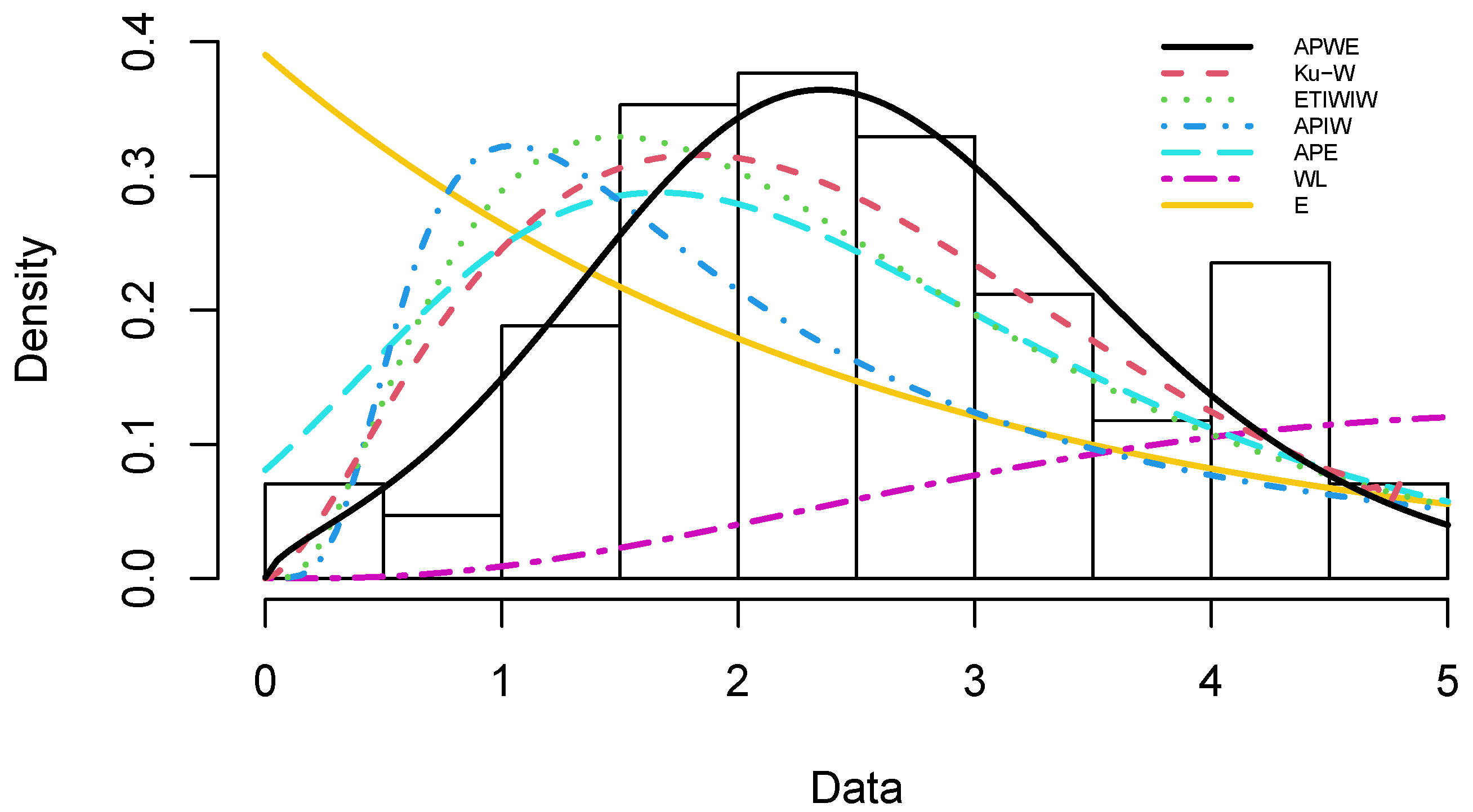
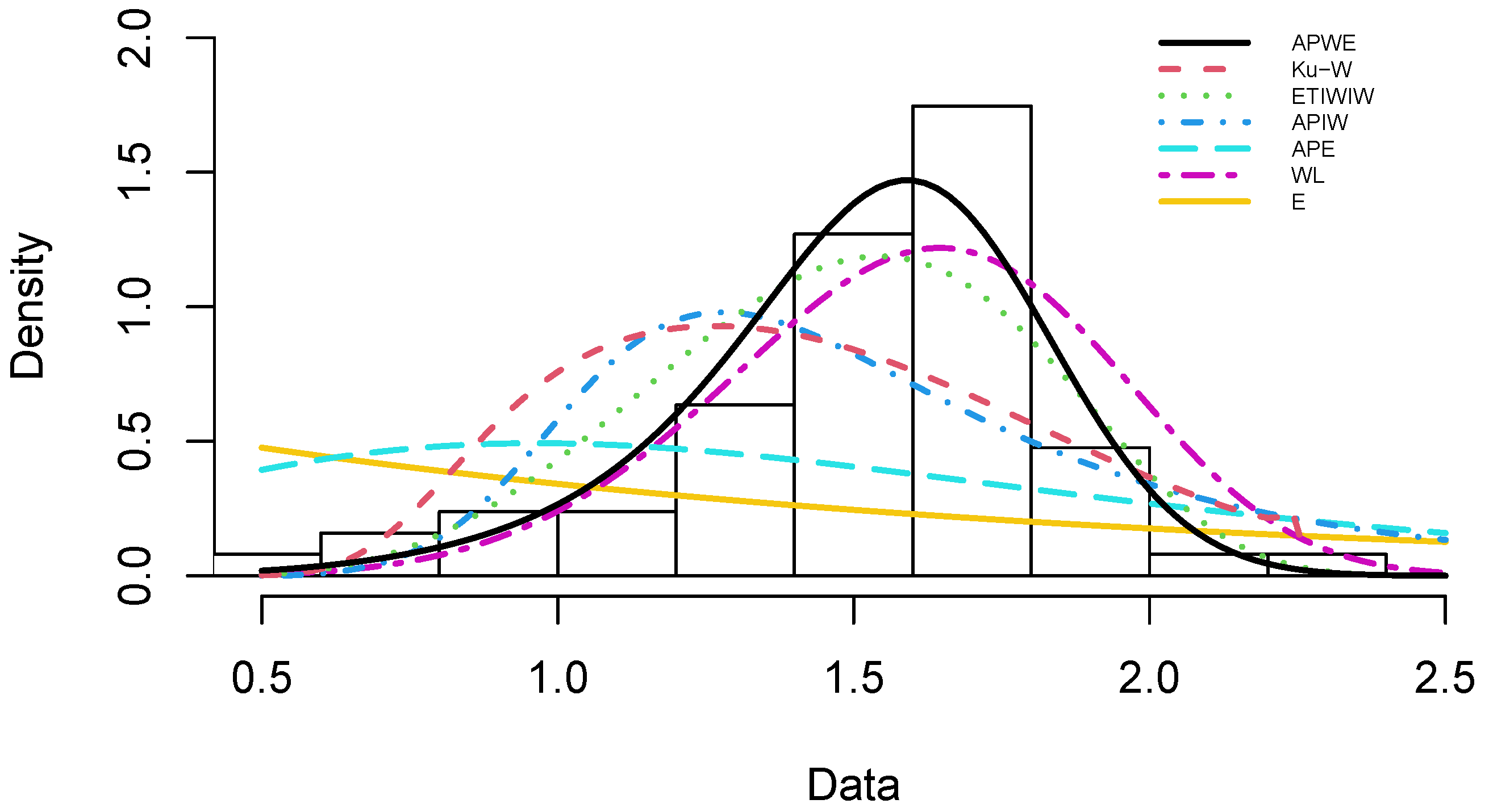
Figure 3, Figure 4 and Figure 5 display the observed density (histogram) for the three real datasets with the estimated PDF of the APWED, along with those of the competing distributions. These figures show that a closer fit to the observed density was provided by the APWED for all datasets.

7. Conclusions

In this article, we introduced a novel approach for generating distributions that provide great flexibility for modeling real data in a variety of fields. The method combines two well-known techniques: T–X and APT. The new distribution, APWED, is introduced as an application of this approach. The density and hazard rate functions of the proposed distribution have appealing shapes for implementing various data behaviors. For example, the APWED can be used to analyze both symmetrical and asymmetrical data shapes. Different fundamental statistical properties of the APWE were provided, such as the moments, quantile, median, mean residual life, order statistics, and entropy. MLEs were obtained for the unknown parameters of the APWED, and the conducted simulation studies showed the consistency and efficacy of the estimators. The application of the new distribution was also demonstrated by fitting three real datasets. The APWED generally provided the best fit, compared to the results of well-known competitive models. Thus, APWED is a promising distribution, which can be used to fit a variety of real-world data.

Author Contributions

Under the idea and supervision of the corresponding author L.A.B., W.H.A. carried out the numerical calculations and a first draft. L.A.B. polished the writing. All authors have read and agreed to the published version of the manuscript.

Funding

This research received no external funding.

Institutional Review Board Statement

Not applicable.

Informed Consent Statement

Not applicable.

Data Availability Statement

Not applicable.

Conflicts of Interest

The authors declare no conflict of interest.

Appendix A. The Partial Derivatives of (33), with Respect to Each Parameter

α = n α + n ( α 1 α log α ) α ( α 1 ) log α 1 α i = 1 n e λ x i γ a ,
λ = n a λ a γ i = 1 n x i λ x i γ a 1 1 log α e λ x i γ a ,
γ = n a γ + a γ i = 1 n λ x i γ a 1 log α e λ x i γ a ,
a = n a + i = 1 n log λ x i γ 1 λ x i γ a + log α λ x i γ a e λ x i γ a .

References

  1. Mudholkar, G.S.; Srivastava, D.K. Exponentiated Weibull family for analyzing bathtub failure-rate data. IEEE Trans. Reliab. 1993, 42, 299–302. [Google Scholar] [CrossRef]
  2. Gupta, R.D.; Kundu, D. Exponentiated exponential family: An alternative to gamma and Weibull distributions. Biom. J. J. Math. Methods Biosci. 2001, 43, 117–130. [Google Scholar] [CrossRef]
  3. Nadarajah, S.; Kotz, S. The exponentiated type distributions. Acta Appl. Math. 2006, 92, 97–111. [Google Scholar] [CrossRef]
  4. Eugene, N.; Lee, C.; Famoye, F. Beta-normal distribution and its applications. Commun. Stat. Theory Methods 2002, 31, 497–512. [Google Scholar] [CrossRef]
  5. Jones, M. Kumaraswamy’s distribution: A beta-type distribution with some tractability advantages. Stat. Methodol. 2009, 6, 70–81. [Google Scholar] [CrossRef]
  6. Alzaatreh, A.; Lee, C.; Famoye, F. A new method for generating families of continuous distributions. Metron 2013, 71, 63–79. [Google Scholar] [CrossRef] [Green Version]
  7. Al-Aqtash, R.; Lee, C.; Famoye, F. Gumbel-Weibull distribution: Properties and applications. J. Mod. Appl. Stat. Methods 2014, 13, 11. [Google Scholar] [CrossRef]
  8. Alzaghal, A.; Famoye, F.; Lee, C. Exponentiated TX family of distributions with some applications. Int. J. Stat. Probab. 2013, 2, 31. [Google Scholar] [CrossRef] [Green Version]
  9. Alzaatreh, A.; Famoye, F.; Lee, C. Weibull-Pareto distribution and its applications. Commun. Stat. Theory Methods 2013, 47, 1673–1691. [Google Scholar] [CrossRef]
  10. Alzaatreh, A.; Famoye, F.; Lee, C. The gamma-normal distribution: Properties and applications. Comput. Stat. Data Anal. 2014, 69, 67–80. [Google Scholar] [CrossRef]
  11. Mahdavi, A.; Kundu, D. A new method for generating distributions with an application to exponential distribution. Commun. Stat. Theory Methods 2017, 46, 6543–6557. [Google Scholar] [CrossRef]
  12. Nassar, M.; Alzaatreh, A.; Mead, M.; Abo-Kasem, O. Alpha power Weibull distribution: Properties and applications. Commun. Stat. Theory Methods 2017, 46, 10236–10252. [Google Scholar] [CrossRef]
  13. Ihtisham, S.; Khalil, A.; Manzoor, S.; Khan, S.A.; Ali, A. Alpha-Power Pareto distribution: Its properties and applications. PLoS ONE 2019, 14, e0218027. [Google Scholar] [CrossRef]
  14. Dey, S.; Nassar, M.; Kumar, D. Alpha power transformed inverse Lindley distribution: A distribution with an upside-down bathtub-shaped hazard function. J. Comput. Appl. Math. 2019, 348, 130–145. [Google Scholar] [CrossRef]
  15. Aldahlan, M.A. Alpha Power Transformed Log-Logistic Distribution with Application to Breaking Stress Data. Adv. Math. Phys. 2020, 2020, 2193787. [Google Scholar] [CrossRef]
  16. Klakattawi, H.S.; Aljuhani, W.H. A New Technique for Generating Distributions Based on a Combination of Two Techniques: Alpha Power Transformation and Exponentiated TX Distributions Family. Symmetry 2021, 13, 412. [Google Scholar] [CrossRef]
  17. Johnson, N.L.; Kotz, S.; Balakrishnan, N. Continuous Univariate Distributions, Volume 2; Wiley: New York, NY, USA, 1995; p. 75. [Google Scholar]
  18. David, H.A.; Nagaraja, H.N. Order statistics. Encyclopedia of Statistical Sciences; John Wiley & Sons: Hoboken, NJ, USA, 2004. [Google Scholar]
  19. Efron, B. Logistic regression, survival analysis, and the Kaplan-Meier curve. J. Am. Stat. Assoc. 1988, 83, 414–425. [Google Scholar] [CrossRef]
  20. Tahir, M.H.; Cordeiro, G.M.; Mansoor, M.; Zubair, M. The Weibull-Lomax distribution: Properties and applications. Hacet. J. Math. Stat. 2015, 44, 461–480. [Google Scholar] [CrossRef]
  21. Smith, R.L.; Naylor, J. A comparison of maximum likelihood and Bayesian estimators for the three-parameter Weibull distribution. J. R. Stat. Soc. Ser. C 1987, 36, 358–369. [Google Scholar] [CrossRef]
  22. Cordeiro, G.M.; Ortega, E.M.; Nadarajah, S. The Kumaraswamy Weibull distribution with application to failure data. J. Frankl. Inst. 2010, 347, 1399–1429. [Google Scholar] [CrossRef]
  23. Almarashi, A.M.; Elgarhy, M.; Jamal, F.; Chesneau, C. The exponentiated truncated inverse Weibull-generated family of distributions with applications. Symmetry 2020, 12, 650. [Google Scholar] [CrossRef] [Green Version]
  24. Basheer, A.M. Alpha power inverse Weibull distribution with reliability application. J. Taibah Univ. Sci. 2019, 13, 423–432. [Google Scholar] [CrossRef] [Green Version]
Figure 1. Plots of the APWED PDF, for some certain values.
Symmetry 13 00726 g001
Figure 2. Plots of the APWED hazard function, for some certain values.
Symmetry 13 00726 g002
Figure 3. Fitted distributions for survival time data.
Symmetry 13 00726 g003
Figure 4. Fitted distributions for failure time data.
Symmetry 13 00726 g004
Figure 5. Fitted distributions for strength data.
Symmetry 13 00726 g005
Table 1. The mean, variance, skewness, and kurtosis of the APWED for certain selected values of the parameters.
α λ γ aMeanVarianceSkewnessKurtosis
0.50.5213.337813.17985.39357.3632
121.59620.79011.89852.1830
230.82980.10181.41051.5306
350.58470.01991.16021.2061
5.560.32460.00441.11481.1478
0.90.5213.895315.57664.62106.1819
121.74520.84971.78662.0266
230.88330.10501.36721.4716
350.60790.01971.14571.1867
5.560.33540.00431.10491.1346
1.50.5214.413617.58374.07885.3732
121.87830.88581.69521.9026
230.93030.10571.32911.4210
350.62810.01921.13221.1689
5.560.34480.00421.09541.1222
20.5214.715018.64603.81924.9917
121.95340.89901.64731.8387
230.95660.10521.30821.3938
350.63920.01881.12441.1588
5.560.34990.00401.08991.1150
2.50.5214.951619.42533.63794.7276
122.01140.90571.61211.7923
230.97670.10451.29251.3734
350.64770.01841.11841.1511
5.560.35380.00391.08561.1095
60.5215.884322.02413.06903.9099
122.23160.90401.49211.6361
231.05190.09851.23671.3019
350.67900.01651.09621.1227
5.560.36830.00351.06961.0890
Table 2. Simulation Study results for the APWED.
Set 1Set 2
Sample SizePar.MLEMSEMLEMSE
30 α 2.94222.12010.38064.1005
λ 0.07550.00104.990123.3080
γ 3.78712.49812.795111.2943
a9.53001.90360.30530.0034
50 α 2.93731.54021.29253.5021
λ 0.07710.00104.424417.3286
γ 3.87012.42632.61418.2774
a9.42251.17670.29890.0021
100 α 2.99610.85050.40010.0795
λ 0.10360.00043.939512.6731
γ 5.18920.95042.40145.3823
a9.09460.48440.29430.0014
150 α 3.00510.70860.39600.0687
λ 0.10450.00043.69209.2768
γ 5.23150.88412.37095.0723
a9.09830.37910.29430.0011
200 α 2.98660.59530.41380.0609
λ 0.10370.00033.49568.3503
γ 5.18820.77472.36424.2086
a9.07700.29350.29550.0009
500 α 2.98960.33200.45470.0524
λ 0.10180.00022.94874.2672
γ 5.09230.43102.10322.4497
a9.03340.13930.29690.0005
Table 3. MLEs (SEs in parentheses) for survival time data.
DistributionEstimated Parameters
APWED0.00970.00212.22581.0213
( α ^ , λ ^ , γ ^ , a ^ )(0.0134)(0.0002)(0.7427)(0.0976)
Ku-W0.97830.08480.39940.5239
( α ^ , β ^ , c ^ , γ ^ )(0.4010)(0.0119)(0.0019)(0.0109)
ETIWIW28.07650.06123.50710.1089
( a ^ , b ^ , θ ^ , μ ^ ) (7.3394)(0.0025)(0.0033)(0.0033)
APIW27.111719.16870.8835-
( α ^ , λ ^ , β ^ ) (20.9187)(6.9268)(0.0772)
APE0.27560.0023--
( α ^ , λ ^ )(0.2311)(0.0004)
WL5.12005.43030.76553.0234
( γ ^ , a ^ , α ^ , β ^ )(6.5560)(0.5031)(0.8938)(0.5809)
E0.0027---
( λ ^ ) (0.0003)
Table 4. MLEs (SEs in parentheses) for failure time data.
DistributionEstimated Parameters
APWED25.66852.68514.97131.5886
( α ^ , λ ^ , γ ^ , a ^ )(40.1965)(199.6717)(369.7458)(0.3246)
Ku-W1.36490.08121.90110.7197
( α ^ , β ^ , c ^ , γ ^ )(0.0095)(0.0089)(0.0040)(0.0045)
ETIWIW2.32493.54890.43905.7867
( a ^ , b ^ , θ ^ , μ ^ ) (0.8317)(0.9676)(0.0619)(2.7310)
APIW3.91520.19481.2339-
( α ^ , λ ^ , β ^ ) (1.2192)(0.0235)(0.0695)
APE34.14280.7591--
( α ^ , λ ^ )(13.3994)(0.0592)
WL9.81704.53205.65551.7000
( γ ^ , a ^ , α ^ , β ^ )(10.0656)(0.3975)(4.8035)(0.0898)
E0.3902---
( λ ^ )(0.0423)
Table 5. MLEs (SEs in parentheses) for strength data.
DistributionEstimated Parameters
APWED10.849410.403914.98544.4840
( α ^ , λ ^ , γ ^ , a ^ )(12.8014)(1625.4758)(2341.4107)(0.7681)
Ku-W8.34400.09232.82880.6285
( α ^ , β ^ , c ^ , γ ^ )(0.6533)(0.0117)(0.0024)(0.0024)
ETIWIW1.076823.96790.97915.8196
( a ^ , b ^ , θ ^ , μ ^ ) (0.4988)(18.3488)(0.2967)(3.0173)
APIW193.06040.63653.8769-
( α ^ , λ ^ , β ^ ) (267.2453)(0.1822)(0.3096)
APE33.04831.2993--
( α ^ , λ ^ )(11.9269)(0.1080)
WL2.75398.71082.80701.0327
( γ ^ , a ^ , α ^ , β ^ )(1.7144)(0.8782)(1.0768)(0.0211)
E0.6636---
( λ ^ )(0.0836)
Table 6. GOF criteria for survival time data.
DistributionAICCAICHQICK-SWA θ ^
APWED751.5332752.3332754.63820.15960.34681.8001371.7666
Ku-W795.5555796.3555798.66050.31650.38081.9230393.7778
ETIWIW753.0122753.8122756.11720.19400.35071.9772372.5061
APIW752.8410753.3116755.16980.19270.49752.5184373.4205
APE757.1062757.3369758.65870.17300.39042.1997376.5531
WL752.0366752.8366755.14160.16200.37661.8987372.0183
E764.0156764.0911764.79190.27630.96384.5921381.0078
Table 7. GOF criteria for failure time data.
DistributionAICCAICHQICK-SWA θ ^
APWED267.4350267.9350271.36500.06520.04780.4565129.7175
Ku-W278.3159278.8159282.24590.12880.09870.9209135.158
ETIWIW303.1870303.6870307.11700.16260.58333.4447147.5935
APIW354.8962355.1925357.84370.26191.26827.6828174.4481
APE281.9912282.1375283.95620.16030.60243.4923138.9956
WL285.1424285.6424289.07240.09160.14921.2825138.5712
E331.9754332.0236332.95790.30322.360711.81164.9877
Table 8. GOF criteria for strength data.
DistributionAICCAICHQICK-SWA θ ^
APWE34.948335.637938.31990.12250.13140.855413.4741
Ku-W66.102666.792269.47420.28450.69433.761329.0513
ETIWIW42.853443.543146.22510.19200.39091.987817.4267
APIW81.772482.179184.30110.21630.86794.989437.8862
APE124.7411124.9411126.42690.33882.469212.37960.3706
WL40.532141.221743.90370.17280.28591.565416.2660
E179.6606179.7262180.50350.41803.861818.42488.8303
Publisher’s Note: MDPI stays neutral with regard to jurisdictional claims in published maps and institutional affiliations.