Abstract
The modulation instability of surface capillary-gravity water waves is analysed in a shear flow model with a tangential discontinuity of velocity. It is assumed that air blows along the surface of the water with a uniform profile in the vertical direction. Such a model, despite its simplicity, plays an important role in hydrodynamics as the reference model for investigating basic physical phenomena of wave–current interactions and acquiring insights into a series of complex phenomena. In certain cases where the wavelength of interfacial perturbations is much bigger than the width of the shear flow profile, the model with the tangential discontinuity in the velocity is adequate for describing physical phenomena at least within limited spatial and temporal frameworks. A detailed analysis of the air-flow conditions under which modulation instability sets in is presented. It is also shown that the interfacial waves are subject to dissipative or radiative instability when negative-energy waves appear at the interface.
1. Introduction
A shear flow with the tangential discontinuity of velocity plays an important role in hydrodynamics, despite the real wind profiles usually being nonuniform; they are often approximated by the logarithmic dependence of wind velocity with height. Nevertheless, a wind flow with the uniform profile plays an important role as it serves as the reference model in the study of the physical phenomena of wave–current interaction and for gaining insights into these complex areas (see [1]). This model is attractive because of its simplicity and richness of the effects. In particular, it can provide simple explanations of the concepts of negative energy waves (NEWs) [2,3], wave-induced currents [2,4], over reflection phenomenon [2,5,6], etc. Furthermore, in the cases where the wavelength of the interfacial perturbations is much greater than the width of the shear flow profile, this model can describe physical phenomena adequately, at least within the limited spatial and temporal frameworks.
As is well-known [7], Kelvin and Helmholtz attempted to explain wave generation by wind with the uniform profile in the inviscid fluids (both in the air and water). However, it was discovered that waves are observed to be generated at wind speed far below the predicted Kelvin–Helmholtz (KH) threshold speed ∼6.7 m/s. In the considered model, the existence of NEWs was missing which do not manifest themselves if dissipation mechanisms are ignored. This concept of NEWs was initiated in hydrodynamics after the pioneering paper by Brooke Benjamin in the early 1960s [8]. However, this concept is not widely understood up to now. As was demonstrated in [2], the existence of NEWs leads to the possibility of shear flow instability for a smaller current speed. In particular, in the K-H model, the potentially unstable (growing with time) NEWs exist as the wind speed exceeds 0.23 m/s. The interplay of the air and water viscosity leads to the threshold speed of wind wave generation up to approximately m/s which agrees rather well with the observations.
The shear-flow model with the tangential discontinuity of velocity has been studied in detail in the linear approximation (see [2]); but to the best of our knowledge, the modulation instability of weakly nonlinear wave trains has not been studied yet. It is of interest to determine the conditions which lead to the modulation instability because generation of quasi-stationary nonlinear wave trains-envelope solitons are expected under such conditions. An ensemble of envelope solitons with random parameters can play an important role in the development of strong wave turbulence at least for moderate wind intensity [9].
The main aim of this paper is to fill up the gap in the study of modulation instability at the air-water interface and to present a detailed analysis of the conditions leading to the modulation instability within the framework of a simplified reference model. Following [10,11], we neglect the viscosity of both air and water to separate the modulation instability per se. The developed approach is suitable, in particular, to superfluids having no viscosity at all.
2. Formulation of the Problem
We consider a shear flow that consists of an upper layer fluid flowing with a uniform velocity over a lower layer fluid of higher density as shown schematically in Figure 1. We assume that both of the layers are of infinite extents in the two-dimensional Cartesian coordinate system. The classical examples are air-flow over a free surface of the water or a motion of one layer of a fluid relative to another layer of a different density. In the present study, the effect of surface tension is taken into consideration at the interface between the fluid layers by assuming that the two fluids are immiscible, and the fluids of both layers are perfect. We choose coordinate axes as shown in Figure 1, with the x-axis being directed along the horizontal direction and the z-axis being directed vertically upward, so that the acceleration due to gravity is directed downward, with the line being along the mean interface.
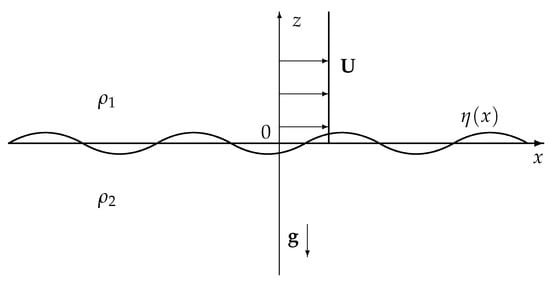
Figure 1.
Sketch of fluid flow in two layers of infinitely deep fluids with an immovable lower layer and tangential discontinuity of velocity in upper layers.
Let be the density of the upper layer fluid, be the density of the lower layer fluid, U be the fluid speed of the upper layer (wind speed), and T be the surface tension at the interface of the two-layers.
The assumption of perfect fluids allows us to introduce hydrodynamic potentials for the perturbed velocities in each layer as , for , where subscript 1 corresponds to the upper layer fluid and the subscript 2 corresponds to the lower layer fluid. The condition of fluid incompressibility yields the Laplace equation for the potential flow in each layer, which is given by the equation:
We assume that there are no wave perturbations far from the interface in the vertical direction as :
The kinematic boundary conditions at the interface are given by the set of equations
where is the perturbation of the interface.
The dynamic boundary condition at the interface yields:
In the linear approximation of wave perturbations of infinitesimal amplitudes, we can seek a solution for the perturbation at the interface in the form:
where stands for the complex-conjugate, and A is a constant.
The perturbations of the velocity potentials in the upper and lower layers, which satisfy the Laplace equations and kinematic boundary conditions as in Equations (4) and (5) in the linear approximation, are given by:
and
The boundary conditions of vanishing perturbations at are taken into account in this approximation. Substituting these solutions into the dynamic boundary condition (6), we obtain the dispersion relation:
Solving the dispersion relation (10) with respect to , we obtain the dependences of the wave frequency on the wavenumber k in the explicit form (as in [2]):
where is the density ratio.
Graphical representations of the dispersion relations for three typical velocities are shown in Figure 2. For the sake of convenience, we assume that wavenumber k is positive and that the frequency is of either sign. However, from the physical point of view, the wave frequency is a positive quantity, whereas the wavenumber k is of either sign being in the interval .
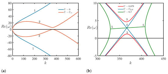
Figure 2.
(Color online.) (a) Dispersion relations for water waves in the cases when U = 0 (line 1) and U = Uc1 = 6.676 m/s (line 2); (b) magnified fragments of the dispersion relations in the vicinity of the critical point at different velocities: U = 6.679 m/s (line 3), U = UKH = 6.68 m/s (line 4), and U = 6.7 m/s (line 5). The figures are plotted for a = 0.0012 and T = 0.073 N/m.
Equation (11) describes the two branches of the dispersion relation that are symmetric with respect to the k-axis for . These branches correspond to capillary-gravity waves travelling in opposite directions with phase speed (Figure 2a).
For , the dispersion curves become non-symmetric because of the wave drift caused by the flow. When U increases and becomes bigger than some critical value , the lower branch of the dispersion curve in Figure 2b changes sign and becomes positive for where
Here, the negative sign pertains to and the positive sign to . The portion of the dispersion curve in Figure 2 where the frequency changes sign corresponds to NEWs [2]. The dispersion curves shown in Figure 2 are presented in Figure 3 for with . In this representation, the wave energy becomes negative when the wave frequency becomes formally negative. However, the waves with ‘negative energy’ are actually captured by a fluid flow and propagate co-current as shown in Figure 3.
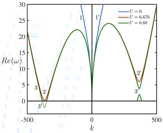
Figure 3.
(Color online.) Dispersion curves of the KH model. Lines 1 and 1 pertain to the case when ; lines 2 and 2 to ; and lines 3 and 3 to . The dashed portion of line 3 corresponds to NEWs, and its counterpart with is shown by the solid line in the right half-plane for .
When U increases further, the two branches of the dispersion curve continue to converge, and eventually reconnect (lines 4 in Figure 2b) when , where , for an air-water interface with , . The KH instability arises when U becomes greater than , and the instability occurs in the interval , where
Such re-connection is typical for the interaction of waves of opposite energy signs [2,3]. Thus, the appearance of the KH instability can be attributed to an interaction of waves of opposite energy signs. The NEWs on the lower branch of the dispersion curve transfer their energy to the positive-energy waves, on the upper branch of the dispersion curve. As a result, the amplitudes of both waves grow with time.
When U is in the interval, , then there is no KH instability; however, there are non-growing but potentially unstable NEWs. Negative energy waves existing in the interval can grow if the associated wave energy is depleted, i.e., if there is a mechanism that draws their energy. It can be easily shown from the expressions for and that these velocities are very close to each other when a is small. This is the case of the air-water interface with . If , which is typical for internal layers in the ocean or atmosphere, then which was initially noted by Benjamin [8]. There are potentially different mechanisms which can cause NEWs to grow. In particular, viscous dissipation in an immovable lower fluid layer leads to the growth of NEWs [12]. This is analogous to dissipative instability in plasma physics [13].
For NEWs to be amplified, the viscosity must lead to ‘positive losses’. For example, NEWs in the model under consideration will be damped if the moving upper layer is viscous rather than the fixed lower layer. However, positive-energy waves can grow on the upper branch of the dispersion curve, since the viscosity of the moving upper layer leads to ‘negative damping’.
Indeed, in passing over to the reference system in which the upper layer is at rest and the lower layer is moving with a uniform speed U, the energy of the growing mode and, simultaneously, the dissipation change their signs [2]. In such a reference system, NEWs exist in the upper branch of the dispersion curve and can grow under the influence of positive dissipation. The shear flow instability associated with this mode does not vary with the reference system. The dispersion relation in the reference frame in which the upper layer is at rest and the lower layer moves with the speed U in the opposite direction can be obtained easily from the dispersion relation (10) by the formal replacement . In this case, NEWs arise when the velocity of the lower layer , where
It may be noted that the difference between the critical velocities and is small if (as in the case of internal waves on the ocean pycnocline), but it is rather significant for (as in the case of air-water interface in which m/s). In general, NEWs can exist on both the branches of the dispersion curves for waves that are slowed down relative to the flow which means their phase velocities being less than the velocities of the corresponding fluid layers.
The dispersion dependence (Equation (11)) can be considered in the ‘mean-mass’ reference frame which is moving with the velocity . In this frame, the lighter fluid in the upper layer moves in the positive direction with velocity the , whilst the heavier fluid in the lower layer moves in the opposite direction with the velocity . In this case, the two branches of the dispersion curves are symmetric relative to the k-axis due to the Doppler frequency shift (Figure 4). It can be noted that there are no NEWs in this reference frame and the dispersion curves do not change their signs.
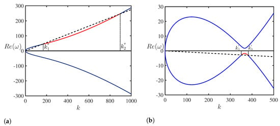
Figure 4.
(Color online.) Dispersion curves for waves at the air–water interface in the ‘mean-mass reference frame’ with (a) U = 0.275 m/s and (b) U = 6.679 m/s. The portions of the dispersion curves corresponding to the retarded waves that can be a subject of instability and are highlighted in red.
For sufficiently large values of U, there are portions on the dispersion curves that correspond to the ‘retarded waves’. The phase speed of these waves is less than the current speed of the corresponding layer. For , the retarded waves appear on the dispersion curve below the dashed straight line (Figure 4). Waves with the wavenumbers in the range , where
have phase speeds in the “mean-mass” reference frame.
With further increase of the current speed, the retarded waves appear for on the lower branch of the dispersion curve; they are shown in Figure 4b above the straight line in a very narrow wavenumber range with being given in Equation (12). It is difficult to demonstrate both the dashed straight lines having different slopes and the portions of dispersion curves corresponding to the retarded waves in the figure as the parameter a is considered to be very small for the air-water interface. For this reason, they are shown in separate frames in Figure 4 with different horizontal and vertical scales.
The estimates for the air-water interface demonstrate that m/s, whereas m/s which is equal to the minimal phase speed of surface waves on quiescent water. For , the air viscosity provides ‘negative dissipation’, which may give rise to the dissipative instability of surface waves [2,3,13]. However, the dissipation in water continues to be positive up to the velocity . Thus, the dissipation in water increases the threshold velocity of the wind and, consequently, delays the onset of instability of wind waves [7].
Furthermore, with the increase in the wind velocity, the effective dissipation in the lower layer fluid changes its sign for and then for with the dispersion branches reconnect, and the KH instability arises (see lines 3, 4 and 5 in Figure 2b). In real conditions, wind wave instability sets in much earlier than the classical KH theory predicts [7], for m/s.
From the aforementioned discussion, it reveals that, for , the heavier lower layer fluid ‘carries’ those surface waves of which the dispersion properties (for ) are perturbed slightly due to the presence of the lighter fluid in the upper layer. Simultaneously, the dissipation in the air which moves faster than certain waves at the interface, leads to instability of surface waves, i.e., to the appearance of wind waves on quiescent water.
3. Modulation Instability of Capillary-Gravity Waves on the Tangential Discontinuity of Wind Speed
3.1. Problem Formulation
In this section, we consider a small perturbation of the air–water interface in the form represented by Equation (7) with the assumption that A is a slowly varying function of x and t. We will seek solutions for the velocity potentials in the same form as in Equations (8) and (9) but with the functions depending nonlinearly on the perturbation of the interface . Using the governing hydrodynamic equations and the boundary conditions at the interface and at , we obtain:
Here, is a small parameter, is the amplitude of the “zero harmonic” (the mean flow generated by the fundamental harmonic in the upper layer), is the amplitude of the second harmonic, is the amplitude of the third harmonic. If we assume that the nonlinearity is weak, so that , then we obtain that basic contribution to the potential function comes from the first term proportional to .
Here, is the amplitude of the “zero harmonic” (the mean flow generated by the fundamental harmonic in the lower layer), is the amplitude of the second harmonic, is the amplitude of the third harmonic. Assuming again that the nonlinearity is weak, we obtain that basic contribution to the potential function comes from the first term proportional to . Therefore, finally, we obtain that the set of Equations (16) and (17) reduces to:
up to the terms of the order of inclusive.
Substituting the solutions for and from Equations (18) and (19) into the dynamic boundary condition (6) and neglecting terms beyond the cubic term, we obtain the following nonlinear equation:
where
In the absence of a flow, with , these expressions reduce to those derived in [14]. The nonlinear terms on the right-hand side of Equation (20) provide both the second harmonic and mean flow generations by a quasi-sinusoidal primary-harmonic wave mode. In the linear approximation, neglecting the terms on the right-hand side of Equation (20), we obtain the dispersion relation (10).
3.2. Derivation of Nonlinear Schrödinger Equation for Interfacial Waves
To derive the nonlinear Schrödinger (NLS) equation, we use the method of multiple scales by introducing the ‘fast’ and ‘slow’ variables:
where represent fast variables, and are slow ones. Thus, the differential operators can be expressed as the derivative expansions:
where and and k are related by the dispersion relation (11). Bearing in mind these series, we can present the linear part of Equation (20) through the operator
which can be expanded in powers of about the point :
so that, in the linear approximation, we have
Next, we present the perturbation expansion of the interface in the form of the series:
Substituting the expressions of Equations (29) and (30) in Equation (20) and equating the terms of equal powers of , we obtain the linear and the successive nonlinear partial differential equations of various orders:
In the lowest-order approximation, we consider a solution for the quasi-monochromatic perturbation with a slowly varying amplitude in the form (cf. Equation (7)):
Similarly, form for is obtained as:
which includes secular terms, corresponding to the factor . To eliminate such terms, we apply the solvability condition:
Now, using the definition of the group velocity in the form:
we can rewrite the solvability condition as:
Thus, with the help of the solvability condition, a uniformly valid expression for is obtained:
Next, using the expression in Equation (21) for , we derive the expression of for both upper and lower branches of the dispersion relation:
In the next approximation of the parameter in Equation (31), the solvability condition for gives:
The solvability condition in Equation (35) yields
which results in the elimination of the terms containing in Equation (38). Setting and , Equation (38) reduces to:
where and Putting a new variable , Equation (40) is rewritten as:
In the next section, we will discuss in detail separately the lower and upper branches of the dispersion relation and derive expressions for the dispersion and nonlinear coefficients P and Q which in turn will determine the condition of modulation instability.
4. Analysis of Modulation Instability at the Air-Water Interface
4.1. NLS Equation and Modulation Instability on the Lower Branch of the Dispersion Relation
Substituting for the wave frequency with the negative sign as per Equation (11), the dispersion coefficient in Equation (40) is obtained in the form:
Proceeding in the similar manner and using the expression for G in Equation (37), the nonlinear coefficient Q in Equation (40) is obtained as:
In particular, for , the well-known coefficients of the NLS equation for surface gravity waves in deep water are obtained [15,16,17]:
More complicated expressions follow from Equations (42) and (43) in the case of capillary-gravity waves (with ) in deep water [10,11,18] for and .
In Figure 5 and Figure 6, the graphs of and are plotted for the lower branch of the dispersion relation for , m/s, and m/s.
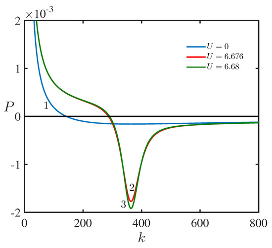
Figure 5.
(Color online.) The dispersion coefficient in the NLS equation as a function of the wavenumber k of the lower branch of the dispersion relation for three different values of the speed of the upper layer fluid with (line 1), m/s (line 2), and m/s (line 3).
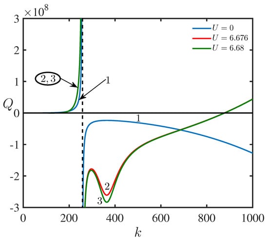
Figure 6.
(Color online.) The nonlinear coefficient in the NLS equation as a function of the wavenumber k for the lower branch of the dispersion relation for three different values of the speed of the upper layer fluid with (line 1), m/s (line 2), and m/s (line 3). Lines 2 and 3 are practically indistinguishable on the left of the dashed vertical line.
As follows from the Lighthill criterion [19,20], a uniform wave train is unstable with respect to self-modulation when the function is positive.
Figure 7 shows zones of modulation stability (S) and instability () in the plane. When , we obtain the well-known diagram of modulation instability of surface waves in deep water [10,11,18]. There is a dramatic change in the stability diagram when U exceeds the critical value m/s.
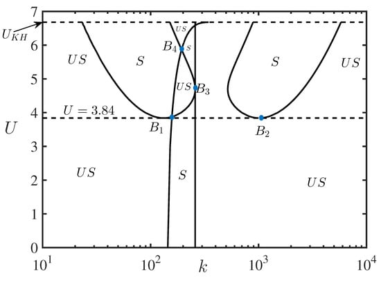
Figure 7.
Zones of modulation stability (S) and instability () in the plane. The dashed line on the top represents the critical velocity m/s when the KH instability arises. The bifurcation points in the diagram are denoted by and for m/s, and two other bifurcation points and are shown for higher values of U.
The maximum of the growth rate of modulation instability occurs when the wavenumber of modulation , where is the amplitude of a sinusoidal wave in the NLS equation as in Equation (41) [21]. The maximal value of the growth rate is . This expression can be further optimized with respect to the carrier wavenumber k for the given value of U. Thus, a maximal possible growth rate of modulation instability for the given amplitude of the carrier wave was obtained.
When the modulation instability occurs, one can expect a spontaneous generation of envelope solitary waves (solitons), breathers, freak waves and other interesting phenomena related to their interactions [17,18,22]. In the case of modulational stability, dark solitons can be formed against a background of quasi-sinusoidal waves [18].
4.2. NLS Equation and Modulation Instability on the Upper Branch of the Dispersion Relation
The similar analysis can be conducted for waves on the upper branch of the dispersion relation in Equation (11) with the upper sign being chosen positive in front of the square root. Thus, the dispersive and nonlinear coefficients of the NLS equation in this case are obtained as:
Figure 8 and Figure 9 demonstrate the the dispersive and nonlinear coefficients P and Q of the NLS equation for the upper branch of the dispersion relation in Equation (11).
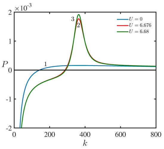
Figure 8.
(Color online.) The dispersion coefficient in the NLS equation as a function of the wavenumber k for the upper branch of the dispersion relation for three different values of the speed of upper layer fluid with (line 1), m/s (line 2), and m/s (line 3).
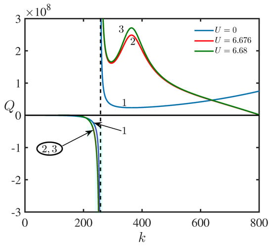
Figure 9.
(Color online.) The nonlinear coefficient in the NLS equation as a function of the wavenumber k for the upper branch of the dispersion relation at three different values of the speed of upper layer fluid, (line 1), m/s (line 2), and m/s (line 3). Lines 2 and 3 are practically indistinguishable on the left of the dashed vertical line.
Next, to demonstrate the occurrence of modulation instability, we define function and show in Figure 10 the zones in the plane where is positive i.e., the zone in which modulation instability occurs.
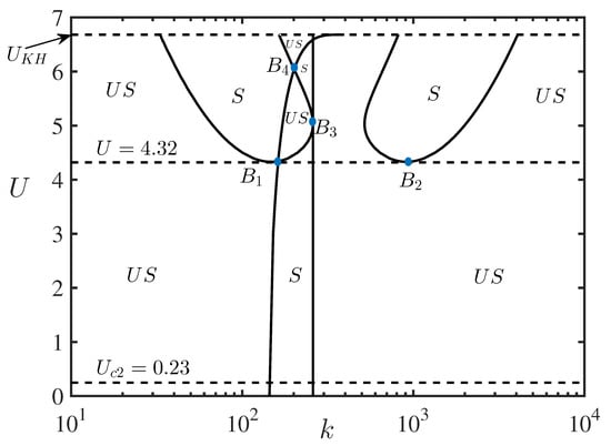
Figure 10.
Zones of modulation stability (S) and instability () in the plane. The dashed line on the top represents the critical velocity m/s when the KH instability arises. The threshold value of m/s, at which NEWs arise, is shown by the lower dashed line. The bifurcation points for m/s are marked by , in the diagram. Two other bifurcation points, and , are shown for the greater values of U.
A comparison of Figure 10 with Figure 7 reveals that a number of stability and instability zones appear when the shear flow exceeds the critical speeds m/s and m/s for the lower and upper branches of the dispersion dependencies, respectively. Interestingly, the stability zones near the edge of the capillary-gravity transition are modified. It becomes the zone of instability, whereas a rather wide stability zone arises in the lower (gravity) range of wavenumbers when U exceeds the corresponding critical values. Moreover, a fairly wide stability zone appears in this case in the capillary range of wavenumbers. To avoid complications in Figure 7 and Figure 10, one can visualize the situation with the transition from instability to stability and again to instability, and so forth by assuming a horizontal cut across these figures at, for example, m/s.
5. Conclusions
In this work, we have studied the modulation stability/instability of surface waves within the simplified model of air-water interface assuming that the air moves relative to water with a uniform velocity profile that does not depend on the height. This is a canonical model of the flow with the tangential velocity discontinuity and such an assumption is widely used in fluid mechanics, physical oceanography, geophysical fluid dynamics, and plasma physics as the model develops insights into the complicated range of phenomena associated with the wave-current interaction. To our best knowledge, the modulation instability of waves within this model has never been attempted in the literature. In this context, the present work has filled the gap in the existing publications and demonstrated the criteria for the occurrence of modulation instability. The diagrams of modulation stability and instability are exhibited graphically for two different branches of the dispersion relation. Known results in the limiting cases of pure gravity waves or capillary-gravity waves without a flow are reproduced from the present model in agreement with the early publications [10,11,18].
The present model has not taken into consideration the influence of viscosity and the dissipative instability of NEWs caused by the air viscosity, as well as wave dissipation in the water. Any dissipative mechanisms have been ignored deliberately to separate the modulation instability per se. From this perspective, we plan to consider viscous and nonlinear effects in the slightly super-critical case when the wind speed is higher than the threshold value for the generation of NEWs. As a result, the narrow-band weakly nonlinear wave trains in the form of the envelope solitons can be generated and grow in time until saturation caused by higher-order nonlinearity and dissipation. The dynamics of ensembles of such solitons and their interaction is a matter of a great interest in different branches of physical sciences associated with the fluid motion in stratified layers. We plan to study the development of dissipative instability and generation of envelop solitons in a separate paper. Similar processes have been studied within the NLS equation with sources and dissipation [2] and with the forcing term [23].
We believe that this model provides, first of all, insights into the modulation instability of waves in shear flows and predicts the existence of multiple zones of stability and instability depending on the intensity of the flow. Apparently, these zones or, at least, some of them still exist within more realistic models with smooth shear flow profiles. The model considered here predicts the ranges of parameters where the modulation instability in the shear flows with smooth profiles can be found. This work provokes further numerical and experimental study to validate the results obtained and observe the generation of envelope solitons in the predicted zones of modulation instability.
Author Contributions
Conceptualization, Y.S.; methodology, T.S.; validation, S.B. and Y.S.; formal analysis, S.B., Y.S. and T.S.; investigation, S.B., Y.S. and T.S.; resources, T.S.; writing–original draft preparation, S.B. and Y.S.; writing–review and editing, T.S. and Y.S.; visualization, T.S.; supervision, T.S. and Y.S.; project administration, T.S. All authors have read and agreed to the published version of the manuscript.
Funding
The authors acknowledge the partial support received from the Ministry of Human Resource and Development, Government of India through Apex Committee of SPARC vide Grant No. SPARC/2018-2019/P751/SL. S.B. acknowledges the financial support received from the Council of Scientific and Industrial Research, New Delhi, India through the senior research fellowship vide file no: 09/081(1345)/2019-EMR-1. Y.S. acknowledges the funding of this study provided by the State task program in the sphere of scientific activity of the Ministry of Science and Higher Education of the Russian Federation (Grant No. FSWE-2020-0007) and the grant of President of the Russian Federation for the state support of Leading Scientific Schools of the Russian Federation (Grant No. NSH-2485.2020.5).
Data Availability Statement
The data are available upon request.
Conflicts of Interest
The authors declare that there is no conflict of interest between them and with any other third parties.
References
- Landau, L.D.; Lifshits, E.M. Fluid Mechanics; Butterworth-Heinemann: Burlington, MA, USA, 1987. [Google Scholar]
- Fabrikant, A.L.; Stepanyants, Y.A. Propagation of Waves in Shear Flows; World Scientific Publishing Company: Singapore, 1998. [Google Scholar]
- Ostrovski, L.A.; Rybak, S.A.; Tsimring, L.S. Negative energy waves in hydrodynamics. Sov. Phys. Uspekhi 1986, 29, 1040. [Google Scholar] [CrossRef]
- Ezersky, A.B.; Ostrovsky, L.A.; Stepanyants, Y.A. Wave-induced flows and their contribution to the energy of wave motions in a fluid. Izv. Acad. Sci. USSR Atmos. Ocean. Phys. 1981, 17, 890–895. [Google Scholar]
- Miles, J.W. On the reflection of sound at an interface of relative motion. J. Acoust. Soc. Am. 1957, 29, 226–228. [Google Scholar] [CrossRef]
- Ribner, H.S. Reflection, transmission and amplification of sound by a moving medium. J. Acoust. Soc. Am. 1957, 29, 435–441. [Google Scholar] [CrossRef]
- Jeffreys, H. On the formation of water waves by wind. Proc. R. Soc. Lond. Ser. A 1925, 107, 189–206. [Google Scholar]
- Benjamin, T.B. The threefold classification of unstable disturbances in flexible surfaces bounding inviscid flows. J. Fluid Mech. 1963, 16, 436–450. [Google Scholar] [CrossRef]
- Gelash, A.; Agafontsev, D.; Zakharov, V.; El, G.; Randoux, S.; Suret, P. Bound state soliton gas dynamics underlying the noise-induced modulational instability. Phys. Rev. Lett. 2019, 123, 890–895. [Google Scholar] [CrossRef] [PubMed]
- Ablowitz, M.J.; Segur, H. On the evolution of packets of water waves. J. Fluid Mech. 1979, 92, 691–715. [Google Scholar] [CrossRef]
- Djordjevic, V.D.; Redekopp, L.G. On two-dimensional packets of capillary–gravity waves. J. Fluid Mech. 1977, 79, 703–714. [Google Scholar] [CrossRef]
- Cairns, R.A. The role of negative energy waves in some instabilities of parallel flows. J. Fluid Mech. 1979, 92, 1–14. [Google Scholar] [CrossRef]
- Nezlin, M.V. Negative-energy waves and the anomalous Doppler effect. Sov. Phys. Uspekhi 1976, 19, 946. [Google Scholar] [CrossRef]
- Abourabia, A.M.; Mahmoud, M.A.; Khedr, G.M. Solutions of nonlinear Schrödinger equation for interfacial waves propagating between two ideal fluids. Can. J. Phys. 2009, 87, 675–684. [Google Scholar] [CrossRef]
- Peregrine, D.H. Water waves, nonlinear Schrödinger equations and their solutions. Anziam J. 1983, 25, 16–43. [Google Scholar] [CrossRef]
- Stiassnie, M. Note on the modified nonlinear Schrödinger equation for deep water waves. Wave Motion 1984, 6, 431–433. [Google Scholar] [CrossRef]
- Yuen, H.C.; Lake, B.M. Nonlinear dynamics of deep-water gravity waves. In Advances in Applied Mechanics; Elsevier: Amsterdam, The Netherlands, 1982; Volume 22, pp. 67–229. [Google Scholar]
- Ablowitz, M.J.; Segur, H. Solitons and the Inverse Scattering Transform; SIAM: Philadelphia, PA, USA, 1981. [Google Scholar]
- Lighthill, M.J. Contributions to the theory of waves in nonlinear dispersive systems. IMA J. Appl. Math. 1965, 1, 269–306. [Google Scholar] [CrossRef]
- Lighthill, M.J. Waves in Fluids; Cambridge University Press: Cambridge, UK, 1978. [Google Scholar]
- Ostrovsky, L.A.; Potapov, A.I. Modulated Waves: Theory and Applications; The Johns Hopkins University Press: London, UK, 1999. [Google Scholar]
- Kharif, C.; Pelinovsky, E.; Slunyaev, A. Rogue Waves in the Ocean; Springer: Berlin/Heidelberg, Germany, 2009. [Google Scholar]
- Slunyaev, A.; Sergeeva, A.; Pelinovsky, E. Wave amplification in the framework of forced nonlinear Schrödinger equation: The rogue wave context. Phys. D 2015, 303, 18–27. [Google Scholar] [CrossRef]


Publisher’s Note: MDPI stays neutral with regard to jurisdictional claims in published maps and institutional affiliations. |
© 2021 by the authors. Licensee MDPI, Basel, Switzerland. This article is an open access article distributed under the terms and conditions of the Creative Commons Attribution (CC BY) license (https://creativecommons.org/licenses/by/4.0/).