Abstract
In relativistic celestial mechanics, post-Newtonian (PN) Lagrangian and PN Hamiltonian formulations are not equivalent to the same PN order as our previous work in PRD (2015). Usually, an approximate Lagrangian is used to discuss the difference between a PN Hamiltonian and a PN Lagrangian. In this paper, we investigate the dynamics of compact binary systems for Hamiltonians and Lagrangians, including Newtonian, post-Newtonian (1PN and 2PN), and spin–orbit coupling and spin–spin coupling parts. Additionally, coherent equations of motion for 2PN Lagrangian are adopted here to make the comparison with Hamiltonian approaches and approximate Lagrangian approaches at the same condition and same PN order. The completely opposite nature of the dynamics shows that using an approximate PN Lagrangian is not convincing. Hence, using the coherent PN Lagrangian is necessary for obtaining an exact result in the research of dynamics of compact binary at certain PN order. Meanwhile, numerical investigations from the spinning compact binaries show that the 2PN term plays an important role in causing chaos in the PN Hamiltonian system.
1. Introduction
The first detection of gravitational waves by LIGO and Virgo confirmed Einstein’s (1915s) theory of general relativity [1,2,3,4,5]. As one of the most important predictions of general relativity, the confirmation of observations for the gravitational wave has opened a new window for studying the universe. Relativistic binary systems are some of the candidates in giving birth to gravitational waves. The post-Newtonian approximation is a better theory for calculating and analyzing gravitational waves to better combine the observed data of gravitational waves. Post-Newtonian theory is undoubtedly a powerful tool in the arsenal of general relativity, and it can make reliable predictions for gravitational experiments. It is surely suitable for describing compact binary systems. In a weak field, the post-Newtonian approximation is a theory for physical systems in which motions are slower than the speed of light c. This can characterize the system as the expansion by a small parameter [6,7,8]. High-precision theoretical templates of gravitational waveforms can be provided by the high post-Newtonian (PN) order. For example, a 4PN one with spin and non-spin evolution was given by a two-body problem [9,10,11,12,13,14].
However, chaos is the hindrance in matching gravitational waveforms [15,16,17,18,19,20]. The initial conditions of the system have a sensitive effect on the emergence of chaos. The maximum Lyapunov exponent is an important tool for distinguishing chaos. It can determine the decay scale of gravitational waves in the near orbit, and this part of the gravitational wave cannot be found by filtering matching [21]. To further investigate the effect of chaos on gravitational waves, the gravitational wave generated by spinning particles rotating around the Kerr black hole was investigated as a classic example. The energy spectrum of gravitational waves showed the obvious difference, and the spectrum of spinning particles is more complicated than that of spinless particles [22]. The chaos of the compact binary system was investigated by Levi and Schnittman [23,24]. Meanwhile, several efforts have been made to overcome this difficulty by our group. Three manifold correction methods were used to preserve all integrals of motion on spinning compact binary, and the second-order implicit midpoint symplectic algorithm was applied to explore the chaos of relativistic spinning compact binary system [25,26]. A study was conducted on the dynamics of two spinning compact binary systems under the PN Lagrangian—one contained the 2PN part and 1.5PN spin–orbit coupling part, and another the 2.5PN spin–orbit part and 2.5PN spin–spin coupling term. They found that the 2.5PN term enhanced the chaos of the system [27]. The role of the spin term in the integrability and dynamics of the 3PN order spinning compact binary of the Hamiltonian system was investigated by Mei et al. [28]. We have studied the effect of spin–spin couplings on the chaos of the double black hole system when that is of the 2PN order [29]. Using the fast Lyapunov exponent, we investigated the dynamics of a compact binary with the considerable mass of one body spinning in the Lagrangian case numerically; it was found that both the PN conservative Lagrangian formula and the PN conservative Hamiltonian formula cannot be chaotic in the Arnowitt–Deser–Misner (ADM)/harmonic coordinates [30].
The Hamiltonian and Lagrangian have a pivotal role in describing the dynamics of physical systems, especially for complex nonlinear cases. In recent years, there has been quite a lot of research in this area. For the nonlinear high-dimensional filtering and non-smooth final value problems, the stochastic Hamiltonian was fully investigated in the latest research [31,32,33,34,35,36,37]. In the recent treatment of variational problems, it has been found that the second-order Lagrangian can act in a well-constrained way. Simultaneously, they can well describe the properties of physical systems in post-Newtonian theory [38,39,40,41].
For the Lagrangian formulation, a compact binary system was investigated which contained two spinning black holes. Moreover, the harmonic-gauge and fractal methods have been used to show the effects on chaotic behavior [23]. Schnittman et al. disagreed with this opinion because of the non-existent positive Lyapunov exponents [42]. However, positive Lyapunov exponents were found in [43,44]; this is a debate, which highlights the Lyapunov exponents resulting in two different claims on the chaotic behavior of comparable mass spinning binaries. As mentioned in [45], this debate was solved because two different approaches to calculating Lyapunov exponents were used in the above papers. Another debate was focused on the dependence of chaos on a certain parameter or initial condition [46,47]. Subsequently, our team explored this debate and found that the two expressions seem to be contradictory on the surface, but they are both correct [48], because the dynamic behavior of a physical system is often determined by a combination of conditions and parameters.
For the PN Hamiltonian formulation, another PN approximation arises: whether it is equivalent to the Lagrangian form with the same order in the depiction of chaotic behavior. That is the third debate, which highlights the existence or absence of chaos in a PN conservative system of two black holes with one body spinning. The harmonic coordinate 2PN Lagrangian approaches with a single spinning body can present chaos in [42,46], whereas the Arnowitt–Deser–Misner (ADM) 2PN Hamiltonian two-black hole was integrable and non-chaotic [42,49]. Immediately thereafter, two different teams explored the equivalence of these two expressions at the 3PN level [50,51,52]. Levin has previously explained the two different statements for the PN approximation and found that these two formulations are not exactly equivalent, but they are approximately related [11].
We revisited the aforementioned topic in previous work. Usually, under the same coordinate gauge, there are differences between the post-Newtonian Hamiltonian and Lagrangian forms of the same order, as we investigated in previous work. For the nPN term, this difference is caused by the truncation of higher-order terms (including the n+1PN term). That means for the PN Lagrangian formulation, where harmonic coordinates are used, the approximation is mainly caused by the substitution of the lower-order acceleration terms for higher-order ones; however, this is not the case in the treatment of the PN Hamiltonian system. In a weak gravitational field, this will not bring a qualitative difference to the physical system. However, this will directly bring essential changes of integrability or non-integrability to the system when there is a strong gravitational field. We have chosen compact binary systems of comparable mass with arbitrary spins in strong gravitational fields. We found that for the 2PN Arnowitt–Deser–Misner Lagrangian formula, the higher-order Hamiltonian form equivalent to it includes many spin–spin couplings, leading to no fifth integral in the ten-dimensional phase space, so it behaves as always integrable. Nevertheless, as there are five constants of motion in the ten-dimensional phase space, the Arnowitt–Deser–Misner Hamiltonian of 2PN is integral and non-chaotic [50]. Theoretically, a lower-order PN Lagrangian formulation from the Euler–Lagrange equation to infinite order is always equivalent to an infinite order PN Hamiltonian. This was discussed in [53] via a special 1PN Lagrangian form, which is about the relativistic restricted three-body problem. For certain initial conditions of compact binary systems with comparable mass, the conservative PN Hamiltonian and Lagrangian forms are both dynamically chaotic [54].
The authors of [55] found that the orbit–spin coupling can make the chaos enhanced without the 1PN and 2PN orbit terms. Later, Huang et al. [56] investigated the 2PN ADM Lagrangian chaotic dynamics of two spinning black holes and made a comparison between the Lagrangian and related Hamiltonian dynamics, in which approximate PN Lagrangian equations of motion were used. Then, we investigated the PN Hamiltonian dynamics of spinning compact binaries, which contained the 1PN, 2PN, and 3PN order spin–orbit couplings. Remarkably, they are all linear functions of spins and momenta due to the absence of the 1PN term. In the transition from Hamilton to the same PN order Lagrangian, there are several additional terms (3PN, 4PN, 5PN, 6PN, and 7PN spin–spin coupling terms) in the Lagrange besides the corresponding original terms [57]. For testing theories that describe a compact binary system whose composition at least includes one compact object, the precession of the pericentre becomes crucial, especially the second order. Recently, a contribution on potentially detectable effects, for instance, the periastron precession at 2PN, was given by Lorenzo Iorio [58,59].
Equations of motion for PN Lagrangian can be derived in two ways. One is an approximate method; another is a coherent method. For the approximate method, it can obtain the total acceleration from the Euler–Lagrangian equation via a truncated term of higher-order acceleration term. In this sense, they are the approximate equations of motion for the PN Lagrangian system. Additionally, the constants of motion are approximately conserved in these equations. For the coherent method, the Euler–Lagrangian equation can also give the consistent equation of motion for a Lagrangian generally. However, these equations are differential equations of generalized momentum, and they are not truncated. In this process, velocity is not used as an integral variable. In order to obtain the algebraic equation of generalized momentum, an iterative method is needed. This is another approach—the coherent 1PN Lagrangian equations of motion, which were put forward by our team [60]. It also remains at the same PN level as the Lagrangian. This kind of equation of motion exactly conserves the constants of motion in the PN Lagrangian formulation, which is the same as the Hamilton equation in the PN Hamilton formulation. In this way, the PN Lagrangian equations of motion are coherent. Then, the dynamics of the 1PN Lagrangian of spinning compact binaries were investigated when quadrupole–monopole interaction contributions were added [61].
In this work, we consider the ADM PN Lagrangian and PN Hamiltonian dynamics of spinning compact binaries of 2PN order. A comparison among the 2PN Lagrangian, the related 2PN Hamiltonian, and the coherent 2PN Lagrangian dynamics will be made, and how the 2PN terms exert an influence on chaos in the PN Hamiltonian and the PN Lagrangian under the coherent equations of motion will be discussed. The paper has been organized as follows. The 2PN Lagrangian formulation and 2PN Hamiltonian formulation are discussed in Section 2. The numerical comparison among the 2PN Lagrangian, the 2PN Hamiltonian, and coherent 2PN Lagrangian dynamics is presented in Section 3, and we focus on the order or chaos of the systems in the same condition and same PN order. The concluding remarks are given in the last section.
2. PN Lagrangian Formulation and PN Hamiltonian Formulation
2.1. PN Lagrangian Formulation
Here, we consider a compact binary system which have masses and of a Lagrangian formulation, including the Newtonian, first and second-order post-Newtonian, and spin–orbit and spin–spin parts. We let ; the system has a total mass ; the reduced mass is ; is the mass ratio; is the mass parameter. We also adopt geometrized unit ; the relative position of body 1 to body 2 is represented as vector . Here, with a radius of is a unit radial vector, and the momenta of body 1 relative to the center is . The two spin vectors are (); their unit vectors and magnitudes are and (). The system can be expressed as the dimensionless conservative 1PN Lagrangian as follows:
where
The second part on the 1PN contribution [55] is given by
When the binaries in Equation (1) are spinning with 1.5PN spin–orbit coupling and 2 PN spin–spin coupling,
where , .
2.1.1. Approximate Equations of Motion for the PN Lagrangian
In a PN Lagrangian , the generalized momentum and Euler–Lagrange equation are expressed as
We derive the 2PN relative acceleration as follows:
where
2.1.2. Coherent Equations of Motion for the PN Lagrangian
As mentioned [60], coherent equations of motion for PN Lagrangian were given by an iterative method. According to the relation of an algebraic equation for the generalized momenta, we take
In addition, is usually satisfied with
We rewrite coherent generalized momentum differential equation at 2PN as
Then, we derive the velocity in the expression of Equation (15).
They conserve the energy integral and the total angular momentum vector as
2.2. PN Hamiltonian Formulation
A 2PN spinning compact binary system of the Hamiltonian formulation is considered; the same condition as the PN Lagrangian is also used here in the ADM coordinates; then we have the following Hamiltonian:
where
The Hamiltonian is the result of [54].
When the two bodies spin, two types of spin contributions are written as
Their expressions are detailed by [62] as follows:
where , .
The second-order PN term is given in [54] as
In this sense, the obtained Hamiltonian becomes
The Lagrangian and Hamiltonian approaches are typically nonequivalent in the same PN order, and therefore, we should focus on the differences between the two cases of and under the coherent equations of motion in dynamics. These issues will be further discussed in detail in the numerical simulations.
3. Numerical Comparisons
We chose the initial conditions as , , . Then, we calculate Equations (9) and (16) or Equation (8) numerically use the eighth and ninth-order Runge–Kutta–Fehlberg integration algorithm RKF8(9). From Figure 1, we find that precision of energy error is achieved of in the coherent equations when we calculate , whereas it is 0.1 in the approximate equations. This scenario means that the coherent equations are really better than the approximate ones used in a physical system. Meanwhile, in the order of magnitude, the coherent equations are many times more accurate than the approximate equations. From Figure 2, we obtain the relations of the errors of the orbital angular momentum, and a very similar result is given as for the energy errors. From the results above, apart from the energy errors, the errors of the orbital angular momentum all present a stark contrast in terms of computational accuracy. From this point forward, to obtain more accurate descriptions, the coherent equations of motion will be a better choice in the application to physical systems. The chaotic dynamics of compact binary systems have since been investigated. As chaos is an attribute of the physical system itself, using an inadequate calculation method will likely lead to the insufficient performance of the system’s properties, especially for highly nonlinear systems, such as compact binary systems, which are extremely sensitive to initial values. Most prominently, the coherent equations of motion can not only achieve high levels of computational accuracy, but also play a useful role in energy conservation.
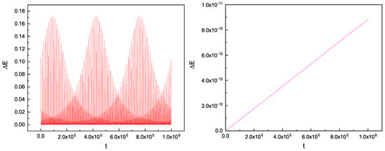
Figure 1.
The post-Newtonian (PN) Lagrangian formulation of nonspinning compact binaries: the left shows the energy errors in the approximate equations of motion, and the right shows in the coherent ones.
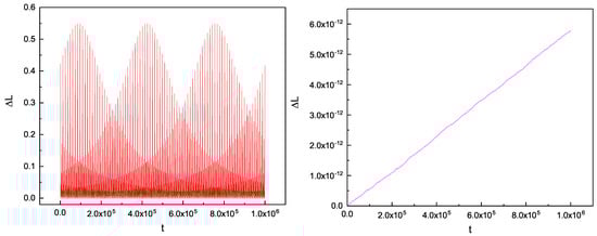
Figure 2.
The PN Lagrangian formulation of nonspinning compact binaries: the left shows the errors of the angular momentum with in the approximate equations of motion, and the right shows in the coherent ones.
Then, we take the mass ratio , dynamical parameters , and initial unit spin vectors.
We investigate dynamical differences among some Lagrangian and Hamiltonian formulations by using several indicators to find chaos.
3.1. Chaos Indicators
A power spectral analysis method can give the distribution of frequencies to a certain time series. It can distinguish between chaotic and ordered orbits preliminarily, based on continuous or discrete spectra. The corresponding orbits will be orderly if the power spectrum is expressed as a discrete spectrum; on the contrary, the corresponding orbit will be chaotic, if the power spectrum is manifested as a continuous spectrum. Here, we use the two subscripts “ex” and “ap” with L to describe the cases in which the form of equations of motion are used; the former is for the coherent, while the latter is the approximate ones.
What shown in Figure 3 corresponding to two sets: (a), (b), and (c) are power spectrums without 2PN term; (d), (e), and (f) are power spectrums added to the 2PN section. In detail, (a) is the case of a Hamiltonian in the first order of a post-Newtonian, (b) and (c) are the same order Lagrangian case, the former corresponds to the approximate method, and the latter is obtained by the coherent equation of motion; similarly, (d) is the power spectrum in the Hamiltonian case when 2PN term is added, (e) and (f) are the same order under the Lagrangian formula; the former uses approximate method, and the latter uses the coherent method. It can be seen from Figure 3 that both (a) and (f) are shown as discrete spectra, so they all indicate that the corresponding orbits are ordered; on the contrary, (b), (c), (d), and (e) all characterize the continuous spectrum; this indicates that their orbits are chaotic. This tell us that the PN Hamiltonian of the 1PN order would manifest regularity in dynamics. Additionally, the 1PN Lagrangians are chaotic with not only the approximate equations of motion but also the coherent ones. The dynamics of PN Hamiltonian and Lagrangian are different in 1PN, but there is an identical dynamical characteristic in the approximate and coherent PN Lagrangian. When we consider an order of 2PN, they are all chaotic in PN Hamiltonian and approximate PN Lagrangian equations. However, the system has a completely different performance when using coherent equations of motion in the PN Hamiltonian. This strongly suggests that using approximate methods to discuss the dynamics of systems is problematic. In addition, when there is a change from 1PN to 2PN for a spinning compact binary system, the PN Hamiltonian becomes chaotic in order, but conversely, the PN Lagrangians all use coherent equations. It has been sufficiently proven that the same orders of PN Lagrangian and Hamiltonian approaches ( and ; and ) have different dynamics. It should be noted that the power spectral approach is unambiguous in distinguishing between complex periodic orbits, quasi-periodic orbits, and weakly chaotic orbits. Therefore, more reliable qualitative methods are necessarily used.
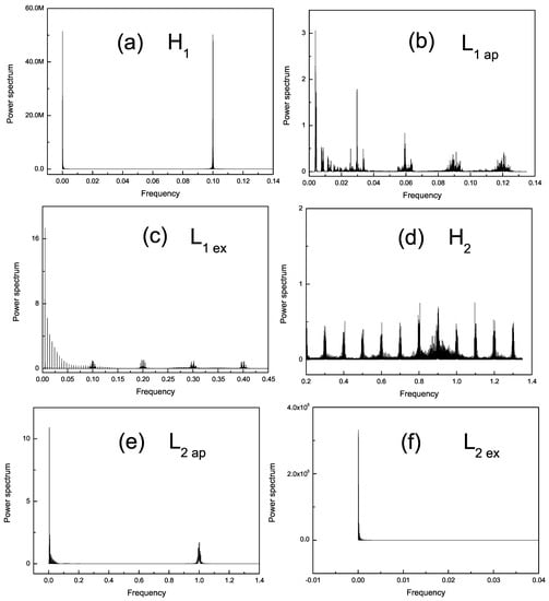
Figure 3.
Power spectra of the PN Hamiltonian formulation and the PN Lagrangian formulation of first and second order. (a) The power spectrum of the 1PN Hamiltonian; (b,c) power spectra under a 1PN Lagrangian; the former uses an approximate method and the latter uses a coherent method; (d) the power spectrum of a 2PN Hamiltonian; (e,f) power spectra under a 2PN Lagrangian; the former uses an approximate method and the latter uses a coherent method.
The Lyapunov exponent is used to measure the average separation rate of two neighboring orbits in the phase space to aid in the quantitative analysis of the strength of chaos. Here, the two-particle method [63], a fitting method, is used in calculating the Lyapunov exponent. The Lyapunov exponent can be defined as
where and are separations between two neighboring orbits at times 0 and t. According to reference [63], for a bounded orbit, it indicates that orbit is chaotic if its Lyapunov exponent is positive; conversely, the orbit is ordered when its Lyapunov exponent tends to zero. We obtain the Lyapunov exponent for the system with and without 2PN in Figure 4, respectively. Additionally, (a) is the case when the 2PN part is not included; (b) is the Lyapunov exponent when the 2PN term is added. From Figure 4a, we find that the Lyapunov exponent in the Lagrangian case with the coherent method is positive at 1PN, which indicates that its corresponding orbit is chaotic, meaning that the dynamics of the system, in this case, exhibit chaotic behavior. However, neither the Hamiltonian case of the same order nor the Lagrangian with the approximation method has a positive Lyapunov exponent and both exhibit convergence to zero. This means that their dynamics are all regular. In Figure 4b, the 2PN term is under consideration. We noticed that the Lyapunov exponent under the Hamiltonian is positive at this time, which corresponds to its chaotic orbits and dynamical behavior. For Lagrangians of the same order, they have Lyapunov exponents that tend to zero regardless of whether the approximation or coherence methods are used, which means that their orbits are ordered. Each case is calculated with time of . In Figure 4a, the system of the PN Hamiltonian formulation corresponds to a regular orbit, and it will tend to be zero with a long integration time. At 1PN, the PN Hamiltonian and coherent Lagrangian have a different dynamical characteristic for a long calculating time; when 2PN is concluded, they are also different dynamically. This indicates that the PN Hamiltonian and Lagrangian are non-equivalent in the same PN order. Note that considerable differences exist in the description of dynamics for PN Hamiltonians and Lagrangians in the same order. Theoretically, the Lyapunov exponents are the limit value, and numerical calculations take a long time to integrate. A more precise tool can be used to better determine the dynamics of physical systems and give an accuracy description for their properties.
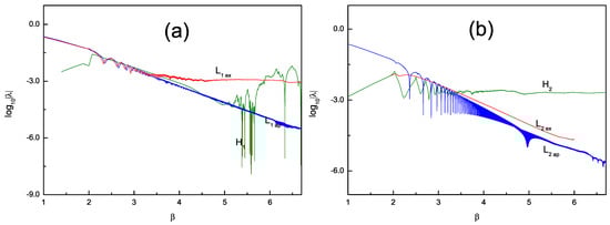
Figure 4.
The Lyapunov exponent of each case. (a) is a comparison among the 1PN Hamiltonian, the 1PN Lagrangian under the approximate method, and the 1PN Lagrangian under the coherent method (, , and ); (b) is a comparison among the 2PN Hamiltonian, the 2PN Lagrangian under the approximate method, and 2PN Lagrangian under the coherent method (, , and ).
A fast Lyapunov indicator (FLI) is a quicker method for finding chaos than the method of Lyapunov exponents. This indicator, which was originally considered to measure the expansion rate of a tangential vector [64], does not need any renormalization, but its modified version can deal with the use of the two-particle method [65]. The FLI is described as
The dynamics of a system can be distinguished as ordered or chaotic for an algebraically or exponentially increase from FLI [65]. That is, the dynamical behavior corresponding to the system is chaotic if the obtained fast Lyapunov indicator grows exponentially with time; conversely, if the fast Lyapunov indicator of the system exhibits an algebraic growth with time, then its dynamical behavior will be ordered. In Figure 5, (a) is the fast Lyapunov indicator obtained when 2PN is not considered, corresponding to the Hamiltonian of 1PN and the Lagrangian of the same order, where the Lagrangian is used in the approximation method and the coherence method, respectively. Similarly, we get (b); the difference is that the 2PN term is included at this point. Note that all the previous cases correspond to fixed mass ratios of compact binary systems. Then, we obtained the fast Lyapunov indicator for the 2PN case after changing the mass ratio for the Hamiltonian and the Lagrangian using the approximation method and the coherence method as in (c). Here, each FLI is obtained after . From Figure 5a, we can see that increases exponentially with , whereas and increase algebraically with time . The FLI of 1PN formulation claims that is chaotic, whereas the and are regular. This is consistent with the results in the Lyapunov exponents above. From Figure 5b, it is clear that corresponds to chaotic orbits, whereas and correspond to regular orbits. Obviously, the dynamical behaviors of the PN Hamiltonian formulation become chaotic more easily when the contribution of the 2PN term is included because the contribution of the 2PN term to the system is mainly in the acceleration part of the system. Moreover, there is another case of FLI for the 2PN Hamiltonian formulation and the 2PN Lagrangian formulation. There is also the evidence that the PN Hamiltonian and coherent PN Lagrangian have different dynamic behaviors, as is shown in Figure 5c for a mass ratio of 1.0. Figure 5b,c indicates that and are always opposite in their dynamics, providing evidence of the non-equivalence between the PN Hamiltonian and the PN Lagrangian formulations. This once again shows the necessity of using the coherent equations of motion to analyze the chaotic behavior of compact binary systems. It should be noted that, unlike in general relativity, we use coordinate distances and time to calculate and FLI in each case. Even so, the dynamical characteristics should correspond to the coordinate distance and time. Given the negligibility of distance and invariant distance herein, the ratio of proper time to coordinate time is not only finite but also positive [66,67].
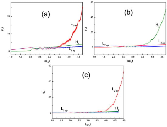
Figure 5.
The fast Lyapunov indicator (FLI) of each case. (a) is a comparison among the 1PN Hamiltonian, the 1PN Lagrangian under the approximate method, and the 1PN Lagrangian under the coherent method (, and ); (b) is a comparison among the 2PN Hamiltonian, the 2PN Lagrangian under the approximate method, and the 2PN Lagrangian under the coherent method (, , and ). (c) is a comparison among , , and when the mass ratio changes to 1.0.
3.2. The Effects of Varying the Mass Ratio on Chaos
As is known to us, the conditions under which chaos occurs in physical systems are numerous and have a very sensitive dependence on the initial conditions. In the previous section on the investigation of the fast Lyapunov indicator, we found that the dynamical behavior of compact binary systems changes as their mass ratios vary. In order to better understand the relationship between the occurrence of chaotic behavior and the mass ratio of a compact binary system, we performed an orbital scan of the system. Here, we held the other values fixed and let change from 0 to 1.4. The values of and FLI correspond to each other when we calculate the time of . In this sense, we obtain Figure 6, where (a) is the result of the fast Lyapunov indicator obtained by scanning when the 2PN term is not considered, containing both the 1PN Hamiltonian and the Lagrangian models using the approximation and coherence methods, respectively. Finally, (b) is the result of scanning the Hamiltonian and the Lagrangian using the two methods when 2PN is included. This is also in the same post-Newtonian order. After extensive numerical calculations, we found that six is a threshold of FLI. For a global stable orbit, it is order or chaos that can be judged by the value of FLI below or higher than six.
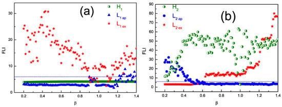
Figure 6.
The FLI as a function of in each case. (a) is a comparison among the 1PN Hamiltonian, the 1PN Lagrangian under the approximate method, and the 1PN Lagrangian under the coherent method (, , and ); (b) is a comparison among the 2PN Hamiltonian, the 2PN Lagrangian under the approximate method, and the 2PN Lagrangian under the coherent method (, , and ).
To distinguish between these two possibilities for the PN Lagrangian and Hamiltonian approximations of the same order, we determine the different dynamical behaviors as a significant measure. Table 1 illustrates the main details of the related differences in terms of chaotic parametric space. It is very clear which case occupies the larger chaotic parameter space under the same conditions. For the first order, the PN Hamiltonian formulation is always regular in space, and the PN Lagrangian formulation with approximate equations of motion has a smaller space of chaotic parameters, indicating a positive effect for the mass ratio to approximate the PN Lagrangian when it is changed from small to large. However, there is a larger space of chaotic parameters for the PN Lagrangian formulation with coherent equations of motion. It has been shown sufficiently that the coherent equations of motion for the PN Lagrangian can describe more completely the dynamics of the system. For the second order, almost the entire interval is covered by the PN Hamiltonian, as there is a clear distinction at approximately 0.60 for the PN Lagrangian in both approximate and coherent forms. The difference is that the coherent PN Lagrangian is starting to become increasingly chaotic at the beginning of 0.60, whereas the approximate one is becoming order. For the attenuation of chaotic behavior, it is not necessarily that chaos goes from strength to weakness. This orbit has the potential to change from order to chaos, or from chaos to order. For example, in Table 1, is order, and is chaotic. Furthermore, the results offer a helpful way to distinguish the PN Hamiltonian and PN Lagrangian with regard to the same order.

Table 1.
Chaotic parameter [0.20,1.40] for systems shown in Figure 6.
4. Summary
There are two approaches to get the equations of motion for the PN Lagrangian. One is the approximate equations of motion of the PN Lagrangian system, which can obtain the total acceleration from the Euler–Lagrangian equation via a truncated term of higher-order acceleration term, and the approximation is mainly caused by the substitution of the lower-order acceleration terms for higher-order ones. Nevertheless, this is not the case in the treatment of the PN Hamiltonian system. The constants of motion are approximately conserved. Another approach is that the Euler–Lagrangian equation can give differential equations of generalized momentum directly. Velocities are not integral variables during this process, but they can be obtained by an iterative method from algebraic equations of generalized momentum. The constants of motion are conserved exactly. Thus, it is the same as the role of Hamilton equations in the post-Newtonian Hamiltonian formulation. In this sense, these equations of motion for the PN Lagrangian are coherent.
In this work, we discussed the comparison of the dynamics of PN Hamiltonians and PN Lagrangians in spinning compact binaries of the same PN order and the same initial condition. We investigated the dynamics of compact binary systems for Hamiltonians and Lagrangians, including Newtonian, post-Newtonian (1PN and 2PN), and spin–orbit coupling and spin–spin coupling parts. Particularly, the coherent equations of motion for PN Lagrangian are used here. The dynamics of systems were considered in three cases, the PN Hamiltonian system, the coherent PN Lagrangian system, and the approximate PN Lagrangian system.
Our numerical analysis shows three points below:
(i) In comparing the dynamical behavior of the approximate PN Lagrangian and coherent PN Lagrangian at the same PN order, we found that they present completely opposite dynamics. As we have discovered, some orbits are ordered under the approximation method, but chaotic under the coherent method; similarly, some orbits are chaotic under the approximation method but ordered under the coherent method. Our numerical results suggest that the non-truncated coherence method of PN Lagrangian is more convincing than the approximate Lagrangian method in discussing PN Hamiltonian and PN Lagrangian dynamics at the same PN order.
(ii) For both the PN Hamiltonian and the coherent PN Lagrangian forms of the same order, they exhibit different dynamical behaviors, which displays they are not equivalent. The nonequivalence is consistent with the results of our previous work in PRD (2015), which compared the PN Hamiltonian and approximate PN Lagrangian forms.
(iii) The 2PN part plays a role in causing the chaos of the PN Hamiltonian, which is also supported by numerical calculations. The characteristic of gravitational waves for different orbits in the two relativistic PN systems of compact binaries will be analyzed in future work.
Author Contributions
The author X.-H.C. had the main idea, organized the literature, made calculations and graphs, and wrote the manuscript. G.-Q.H. contributed to the main idea together, provided the calculations, and checked part of the calculations. All authors have read and agreed to the published version of the manuscript.
Funding
This work was supported by the National Natural Science Foundation of China under grant numbers 11533004, 13008247, and 11563006.
Institutional Review Board Statement
Not applicable.
Informed Consent Statement
Not applicable.
Data Availability Statement
Not applicable.
Conflicts of Interest
The authors declare no conflict of interest.
References
- Abbott, B.P. Observation of Gravitational Waves from a Binary Black Hole Merger. Phys. Rev. Lett. 2016, 116, 061102. [Google Scholar] [CrossRef]
- Buonanno, A.; Chen, Y. Quantum noise in second generation, signal-recycled laser interferometric gravitational-wave detectors. Phys. Rev. D 2001, 64, 042006. [Google Scholar] [CrossRef]
- Kidder, L.E. Coalescing binary systems of compact objects to (post)5/2-Newtonian order. V. Spin effects. Phys. Rev. D 1995, 52, 821–847. [Google Scholar] [CrossRef] [PubMed]
- Thorne, K.S.; Hartle, J.B. Laws of motion and precession for black holes and other bodies. Phys. Rev. D 1985, 31, 1815–1837. [Google Scholar] [CrossRef]
- Cervantes-Cota, C.L.; Galindo-Uribarri, S.; Smoot, G.F. A brief history of gravitational waves. Universe 2016, 2, 22. [Google Scholar] [CrossRef]
- Asada, H.; Futamase, T. Post-Newtonian ApproximationIts Foundation and Applications. Prog. Theor. Phys. Suppl. 1997, 128, 123–181. [Google Scholar] [CrossRef]
- Blanchet, L. Post-Newtonian theory and its application. arXiv 2003, arXiv:gr-qc/0304014. [Google Scholar]
- Will, C.M. On the unreasonable effectiveness of the post-Newtonian approximation in gravitational physics. Proc. Natl. Acad. Sci. USA 2011, 108, 5938–5945. [Google Scholar] [CrossRef] [PubMed]
- Levi, M. Binary dynamics from spin1-spin2 coupling at fourth post-Newtonian order. Phys. Rev. D 2012, 85, 064043. [Google Scholar] [CrossRef]
- Damour, T.; Jaranowski, P.; Schäfer, G. Nonlocal-in-time action for the fourth post-Newtonian conservative dynamics of two-body systems. Phys. Rev. D 2014, 89, 064058. [Google Scholar] [CrossRef]
- Levi, M.; Steinhoff, J. Equivalence of ADM Hamiltonian and Effective Field Theory approaches at next-to-next-to-leading order spin1-spin2 coupling of binary inspirals. J. Cosmol. Astropart. Phys. 2014, 2014, 003. [Google Scholar] [CrossRef]
- Levi, M.; Steinhoff, J. Spinning gravitating objects in the effective field theory in the post-Newtonian scheme. J. High Energy Phys. 2015, 2015, 219. [Google Scholar] [CrossRef]
- Levi, M.; Steinhoff, J. Leading order finite size effects with spins for inspiralling compact binaries. J. High Energy Phys. 2015, 2015, 59. [Google Scholar] [CrossRef]
- Levi, M.; Steinhoff, J. Next-to-next-to-leading order gravitational spin-squared potential via the effective field theory for spinning objects in the post-Newtonian scheme. J. Cosmol. Astropart. Phys. 2016, 2016, 008. [Google Scholar] [CrossRef]
- Varvoglis, H.; Papadopoulos, D. Chaotic interaction of charged particles with a gravitational wave. Astron. Astrophys. 1992, 261, 664–670. [Google Scholar]
- Letelier, P.; Vieira, W. Chaos in black holes surrounded by gravitational waves. Class. Quantum Gravity 1997, 14, 1249. [Google Scholar] [CrossRef]
- Veselỳ, K.; Podolskỳ, J. Chaos in a modified Hénon–Heiles system describing geodesics in gravitational waves. Phys. Lett. A 2000, 271, 368–376. [Google Scholar] [CrossRef]
- Kiuchi, K.; Koyama, H.; Maeda, K.I. Gravitational wave signals from a chaotic system: A point mass with a disk. Phys. Rev. D 2007, 76, 024018. [Google Scholar] [CrossRef]
- Wang, Y.; Wu, X. Gravitational Waves from a Pseudo-Newtonian Kerr Field with Halos. Commun. Theor. Phys. 2011, 56, 1045–1051. [Google Scholar] [CrossRef]
- Wang, Y.; Wu, X.; Zhong, S.Y. Gravitational wave signatures of rotating dense binaries. Acta Phys. Sin. 2012, 61, 16. [Google Scholar]
- Cornish, N.J. Chaos and gravitational waves. Phys. Rev. D 2001, 64, 084011. [Google Scholar] [CrossRef]
- Kiuchi, K.; Maeda, K.I. Gravitational waves from a chaotic dynamical system. Phys. Rev. D 2004, 70, 064036. [Google Scholar] [CrossRef]
- Levin, J. Gravity waves, chaos, and spinning compact binaries. Phys. Rev. Lett. 2000, 84, 3515. [Google Scholar] [CrossRef] [PubMed]
- Schnittman, J.D.; Rasio, F.A. Ruling out chaos in compact binary systems. Phys. Rev. Lett. 2001, 87, 121101. [Google Scholar] [CrossRef] [PubMed]
- Zhong, S.Y.; Wu, X. Manifold corrections on spinning compact binaries. Phys. Rev. D 2010, 81, 104037. [Google Scholar] [CrossRef]
- Zhong, S.Y.; Wu, X.; Liu, S.Q.; Deng, X.F. Global symplectic structure-preserving integrators for spinning compact binaries. Phys. Rev. D 2010, 82, 124040. [Google Scholar] [CrossRef]
- Wang, Y.; Wu, X. Next-order spin–orbit contributions to chaos in compact binaries. Class. Quantum Gravity 2011, 28, 025010. [Google Scholar]
- Mei, L.; Ju, M.; Wu, X.; Liu, S. Dynamics of spin effects of compact binaries. Mon. Not. R. Astron. Soc. 2013, 435, 2246–2255. [Google Scholar] [CrossRef]
- Huang, G.; Ni, X.; Wu, X. Chaos in two black holes with next-to-leading order spin–spin interactions. Eur. Phys. J. C 2014, 74, 1–8. [Google Scholar] [CrossRef][Green Version]
- Wu, X.; Huang, G. Ruling out chaos in comparable mass compact binary systems with one body spinning. Mon. Not. R. Astron. Soc. 2015, 452, 3167–3178. [Google Scholar] [CrossRef][Green Version]
- Ibrahim, D.; Abergel, F. Non-linear filtering and optimal investment under partial information for stochastic volatility models. Math. Methods Oper. Res. 2018, 87, 311–346. [Google Scholar] [CrossRef]
- De Vecchi, F. Lie Symmetry Analysis and Geometrical Methods for Finite and Infinite Dimensional Stochastic Differential Equations. Ph.D. Thesis, Università Degli Studi di Milano, Milano, Italy, 2018. [Google Scholar]
- Germ, F. Estimation for Linear and Semi-Linear Infinite-Dimensional Systems. Master’s Thesis, University of Waterloo, Waterloo, ON, Canada, 2019. [Google Scholar]
- Mirebeau, J.M.; Portegies, J. Hamiltonian fast marching: A numerical solver for anisotropic and non-holonomic eikonal PDEs. Image Process. Line 2019, 9, 47–93. [Google Scholar] [CrossRef]
- Holler, M.; Weinmann, A. Non-smooth variational regularization for processing manifold-valued data. In Handbook of Variational Methods for Nonlinear Geometric Data; Springer: Berlin/Heidelberg, Germany, 2020; pp. 51–93. [Google Scholar]
- Chen, C.; Cohen, D.; D’Ambrosio, R.; Lang, A. Drift-preserving numerical integrators for stochastic Hamiltonian systems. Adv. Comput. Math. 2020, 46, 1–22. [Google Scholar] [CrossRef]
- Sun, W.; Qiu, M.; Lv, X. H filter design for a class of delayed Hamiltonian systems with fading channel and sensor saturation. AIMS Math. 2020, 5, 2909–2922. [Google Scholar] [CrossRef]
- Treanţă, S. Constrained variational problems governed by second-order Lagrangians. Appl. Anal. 2020, 99, 1467–1484. [Google Scholar] [CrossRef]
- Treanţă, S. On a modified optimal control problem with first-order PDE constraints and the associated saddle-point optimality criterion. Eur. J. Control 2020, 51, 1–9. [Google Scholar] [CrossRef]
- Udriste, C.; Pitea, A. Optimization problems via second order Lagrangians. Balk. J. Geom. Appl. 2011, 16, 174–185. [Google Scholar]
- Machado, L.; Abrunheiro, L.; Martins, N. Variational and Optimal Control Approaches for the Second-Order Herglotz Problem on Spheres. J. Optim. Theory Appl. 2019, 182, 965–983. [Google Scholar] [CrossRef]
- Damour, T.; Jaranowski, P.; Schäfer, G. Equivalence between the ADM-Hamiltonian and the harmonic-coordinates approaches to the third post-Newtonian dynamics of compact binaries. Phys. Rev. D 2001, 63, 044021. [Google Scholar] [CrossRef]
- Cornish, N.J.; Levin, J. Comment on “Ruling out chaos in compact binary systems”. Phys. Rev. Lett. 2002, 89, 179001. [Google Scholar] [CrossRef]
- Cornish, N.J.; Levin, J. Chaos and damping in the post-Newtonian description of spinning compact binaries. Phys. Rev. D 2003, 68, 024004. [Google Scholar] [CrossRef]
- Wu, X.; Xie, Y. Revisit on “Ruling out chaos in compact binary systems”. Phys. Rev. D 2007, 76, 124004. [Google Scholar] [CrossRef]
- Levin, J. Fate of chaotic binaries. Phys. Rev. D 2003, 67, 044013. [Google Scholar] [CrossRef]
- Hartl, M.D.; Buonanno, A. Dynamics of precessing binary black holes using the post-Newtonian approximation. Phys. Rev. D 2005, 71, 024027. [Google Scholar] [CrossRef]
- Wu, X.; Xie, Y. Resurvey of order and chaos in spinning compact binaries. Phys. Rev. D 2008, 77, 103012. [Google Scholar] [CrossRef]
- de Andrade, V.C.; Blanchet, L.; Faye, G. Third post-Newtonian dynamics of compact binaries: Noetherian conserved quantities and equivalence between the harmonic-coordinate and ADM-Hamiltonian formalisms. Class. Quantum Gravity 2001, 18, 753. [Google Scholar] [CrossRef]
- Wu, X.; Mei, L.; Huang, G.; Liu, S. Analytical and numerical studies on differences between Lagrangian and Hamiltonian approaches at the same post-Newtonian order. Phys. Rev. D 2015, 91, 024042. [Google Scholar] [CrossRef]
- Königsdörffer, C.; Gopakumar, A. Post-Newtonian accurate parametric solution to the dynamics of spinning compact binaries in eccentric orbits: The leading order spin-orbit interaction. Phys. Rev. D 2005, 71, 024039. [Google Scholar] [CrossRef]
- Gopakumar, A.; Königsdörffer, C. Deterministic nature of conservative post-Newtonian accurate dynamics of compact binaries with leading order spin-orbit interaction. Phys. Rev. D 2005, 72, 121501. [Google Scholar] [CrossRef]
- Chen, R.C.; Wu, X. A note on the equivalence of post-Newtonian Lagrangian and Hamiltonian formulations. Commun. Theor. Phys. 2016, 65, 321. [Google Scholar] [CrossRef]
- Wu, X.; Xie, Y. Symplectic structure of post-Newtonian Hamiltonian for spinning compact binaries. Phys. Rev. D 2010, 81, 084045. [Google Scholar] [CrossRef]
- Wang, H.; Huang, G.Q. The Effect of Spin-Orbit Coupling and Spin-Spin Coupling of Compact Binaries on Chaos. Commun. Theor. Phys. 2015, 64, 159–165. [Google Scholar] [CrossRef]
- Huang, L.; Wu, X.; Ma, D. Second post-Newtonian Lagrangian dynamics of spinning compact binaries. Eur. Phys. J. C 2016, 76, 1–10. [Google Scholar] [CrossRef]
- Huang, L.; Wu, X.; Mei, L.J.; Huang, G.Q. Dynamics of High-Order Spin-Orbit Couplings about Linear Momenta in Compact Binary Systems. Commun. Theor. Phys. 2017, 68, 375. [Google Scholar] [CrossRef]
- Iorio, L. Revisiting the 2PN Pericenter Precession in View of Possible Future Measurements. Universe 2020, 6, 53. [Google Scholar] [CrossRef]
- Iorio, L. On the 2PN Pericentre Precession in the General Theory of Relativity and the Recently Discovered Fast-Orbiting S-Stars in Sgr A. Universe 2021, 7, 37. [Google Scholar] [CrossRef]
- Li, D.; Wang, Y.; Deng, C.; Wu, X. Coherent post-Newtonian Lagrangian equations of motion. Eur. Phys. J. Plus 2020, 135, 390. [Google Scholar] [CrossRef]
- Li, D.; Wu, X.; Liang, E. Effect of the Quadrupole–Monopole Interaction on Chaos in Compact Binaries. Ann. Der Phys. 2019, 531, 1900136. [Google Scholar] [CrossRef]
- Nagar, A. Effective one-body Hamiltonian of two spinning black holes with next-to-next-to-leading order spin-orbit coupling. Phys. Rev. D 2011, 84, 084028. [Google Scholar] [CrossRef]
- Tancredi, G.; Sánchez, A.; Roig, F. A comparison between methods to compute Lyapunov exponents. Astron. J. 2001, 121, 1171. [Google Scholar] [CrossRef]
- Froeschlé, C.; Lega, E. On the structure of symplectic mappings. The fast Lyapunov indicator: A very sensitive tool. In New Developments in the Dynamics of Planetary Systems; Springer: Berlin/Heidelberg, Germany, 2001; pp. 167–195. [Google Scholar]
- Wu, X.; Huang, T.Y.; Zhang, H. Lyapunov indices with two nearby trajectories in a curved spacetime. Phys. Rev. D 2006, 74, 083001. [Google Scholar] [CrossRef]
- Wu, X. A new interpretation of zero Lyapunov exponents in BKL time for Mixmaster cosmology. Res. Astron. Astrophys. 2010, 10, 211. [Google Scholar] [CrossRef]
- Huang, G.; Wu, X. Dynamics of a test particle around two massive bodies in decay circular orbits. Gen. Relativ. Gravit. 2014, 46, 1798. [Google Scholar] [CrossRef]


Publisher’s Note: MDPI stays neutral with regard to jurisdictional claims in published maps and institutional affiliations. |
© 2021 by the authors. Licensee MDPI, Basel, Switzerland. This article is an open access article distributed under the terms and conditions of the Creative Commons Attribution (CC BY) license (https://creativecommons.org/licenses/by/4.0/).