Abstract
The problem of dynamic adaptation of prediction algorithms in chaotic environments based on identification of the situations-analogs in the database of retrospective observations is considered. Under conditions of symmetrical and unsymmetrical chaotic dynamics, traditional computational schemes of precedent prediction turn out to be ineffective. In this regard, a dynamic adaptation of precedent analysis algorithms based on the method of evolutionary modeling is proposed. Implementation of the computational precedent prediction scheme for chaotic processes as well as the evolutionary modeling method are described.
1. Introduction
The state evolution of a controlled object immersed in an instable medium is described by an additive two-parameter model with a system component (represented by the realization of dynamic chaos) and a random component (represented by a nonstationary stochastic process). Such dynamics are quite typical, for example, for turbulent gas-dynamic and hydrodynamic media [1,2,3,4,5,6]. The presence of a chaotic component in the series of observations significantly hinders the prediction problem, because it contradicts the basic assumption of the probabilistic-statistical paradigm. Symmetry can play an important role in the prediction of nonlinear systems. This implies the repeatability of the experimental conditions under identical conditions. As a result, standard extrapolation computational forecasting schemes based on statistical data analysis are ineffective.
An alternative method based on the precedent data analysis was introduced in [7]. This approach represents the generalization of the nearest neighbor method [8,9,10,11,12] and relies on machine learning techniques and pattern recognition [13,14,15]. The precedent data analysis is based on the hypothesis that if the situation, which is similar to the current situation, has occurred before, the consequences can be used as predictive scenarios. This approach is close to the processes, which takes place in human consciousness, and is applicable to many artificial intelligence tasks.
However, due to the weak recurrence of processes in chaotic environments, the proposed method cannot provide a high reliability of the prediction. In this regard, this work proposes an improved version of precedent analysis, based on dynamic adaptation of the precedent detection algorithm. A modified method of evolutionary modeling proposed in [16] is used as an adaptation mechanism, which has found application in many data analysis problems [17,18,19,20].
2. Materials and Methods
The time series of observations , formed by the monitoring system of a real physical process, which takes place in an unstable environment, is used as the initial data for the problem to be solved.
Traditional models of direct observations of the dynamic system state can be described by the additive relation of the following form,
where the system component is an unknown deterministic process to be identified, and is a random process which simulates system noise or measurement errors.
Assumptions concerning the probabilistic nature of the noise component are acceptable in many applications. In particular, the typical assumptions are about the stationarity, ergodicity, independence, and Gaussianity of the process . In order to justify the normality of the distribution, references to the central limit theorems of probability theory are usually used [21,22].
If the above-mentioned conditions are fulfilled, then recovery of a system component is reduced to a procedure of sequential estimation of model parameters based on well-known methods of statistical data analysis—the least squares method, maximum likelihood method, etc. The mathematical structure of the model is specified sequentially, if necessary. The value of , where is the forecast interval, is used as a prognosis of the system state at the moment of time .
The fundamental differences of observation series (1), which are typical for the considered problem, are
- -
- the system component of the observed process represents a realization of dynamic chaos and usually takes the form of an oscillatory non-periodic process with a set of false local trends of indefinite duration and
- -
- the noise component of the observed process is a nonstationary heteroscedastic process with a non-degenerate autocorrelation function that is time-dependent.
Under these conditions, traditional statistical estimates of model parameters not only lose their effectiveness, but may not be valid at all [23,24].
In this regard, an approach based on the precedent analysis of data was proposed [7]. It is based on the typical approach of epistemology, based on the assumption that identical dynamic states of the system correspond to statistically similar after-effects.
To describe the current dynamic state of the controlled object a sliding observation window is used
covering both the current observation and previous samples.
The size of the observation window in traditional statistical studies is estimated based on the minimization of the total error squared, including both the standard deviation and the magnitude of the bias due to dynamic errors. However, this approach is unacceptable for chaotic environments due to the non-stationarity of the observational series. The value of the state window should be considered as an option to be specified during model adaptation.
The search for analogous situations is performed by sequentially browsing the retrospective database with a sliding scan window:
where is the size of the retrospective database used to locate the analogs.
During the scanning process, the search of analogs with the numbers corresponding to the smallest values of the similarity measure is performed. The scanning window with the minimum value of similarity metrics is considered as a precedent.
As such similarity measures, distances of the standard deviation
or the mean absolute deviation are used
It should be noted that in cases (4) and (5), the centered values of observations (CVO) in windows (2) and (3) are used. In addition, in the case of significant heteroscedasticity of the observed process, it is advisable to normalize the state and scanning windows by the estimates of the standard deviation.
In some problems, which are focused on estimation of a local trend, the difference between the coefficients of linear approximation of the observation series in windows (2) and (3) can serve as a measure of similarity:
The aftereffect with following precedent window is used as a prediction:
i.e., behind the scanning window with the minimum value of the selected metric,
The probability of several equal minima is very low. It is only possible at a rough meshing. In this case any minimum can be used as a precedent indicator. To increase the stability of the predicted result, the average value of aftereffects, which follow the obtained windows-analogs, can be used as a prediction
A natural generalization of the prediction (9) is a weighted averaging proportional to the degree of relative similarity with respect to the best result (precedent).
It is impossible to obtain analytical relations for estimating the prediction efficiency in the chosen class of observational series due to the infinite variety of possible variations of the chaotic process. In this connection, the results of numerical studies were presented in [7], which showed a relatively low prediction accuracy. In particular, even in the best case for averaging over analogs, the relative accuracy of the prediction over an interval of 200 min fluctuates around 10–25%.
A variant of developing the precedent prediction based on dynamic adaptation of the model parameters and structure at each step of the prediction is proposed. The fullest degree of optimization adaptation is given by the method of full enumeration of values of model parameters in the range of their admissible variations. The total number of variants for such a run is determined by the number of model parameters and the number of variants for the value of each of the adapted parameters Obviously, with an increase in the parameters number and the accuracy of their determination, the computation amount increases exponentially. The solution of the problem becomes problematic, even for modern computers.
A possible alternative to the full search is based on a random search in space of parameter values. However, this method is characterized by a rather slow convergence and does not guarantee finding the best variant for multidimensional problems.
In the present work, algorithms of the evolutionary modeling method, adapted for specifics of the precedent prediction problem under chaotic dynamics, are used as the main tool for dynamic adaptation.
3. Results and Discussion
3.1. Implementation of the Computational Precedent Prediction Scheme for Chaotic Processes
As an example of the implementation of a precedent prediction scheme, the problem of predicting a series of observational variations in the normalized density of turbulent flow is considered (Figure 1). The “star” symbol divides the process into two parts. The first part with an interval of 200 days is used as a database of retrospective data, designed to search for analogous situations. The second part with an interval of 100 days is used to test the prediction algorithm.
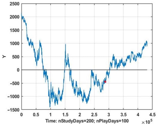
Figure 1.
Time series graph of chaotic process observations.
The precedent prediction is implemented according to the following algorithm:
1. At each k-th step of the prediction the current state window (2) with length of L samples is formed.
2. Using a sliding observation window the whole volume of the retrospective data base is scanned, forming an array of similarity metrics values . Ratios (4)–(6) or other known similarity metrics ratios [8,9,10] are used for metrics calculation.
3. According to (8), the scanning window corresponding to the minimum value of similarity metrics is found. Subsequent sequence (7) of length in samples is taken as a prediction for the k-th situation.
4. Prediction refinement can be carried out on the basis of (9) by averaging of the aftereffects for the situation-analogs with the lowest values of similarity metrics.
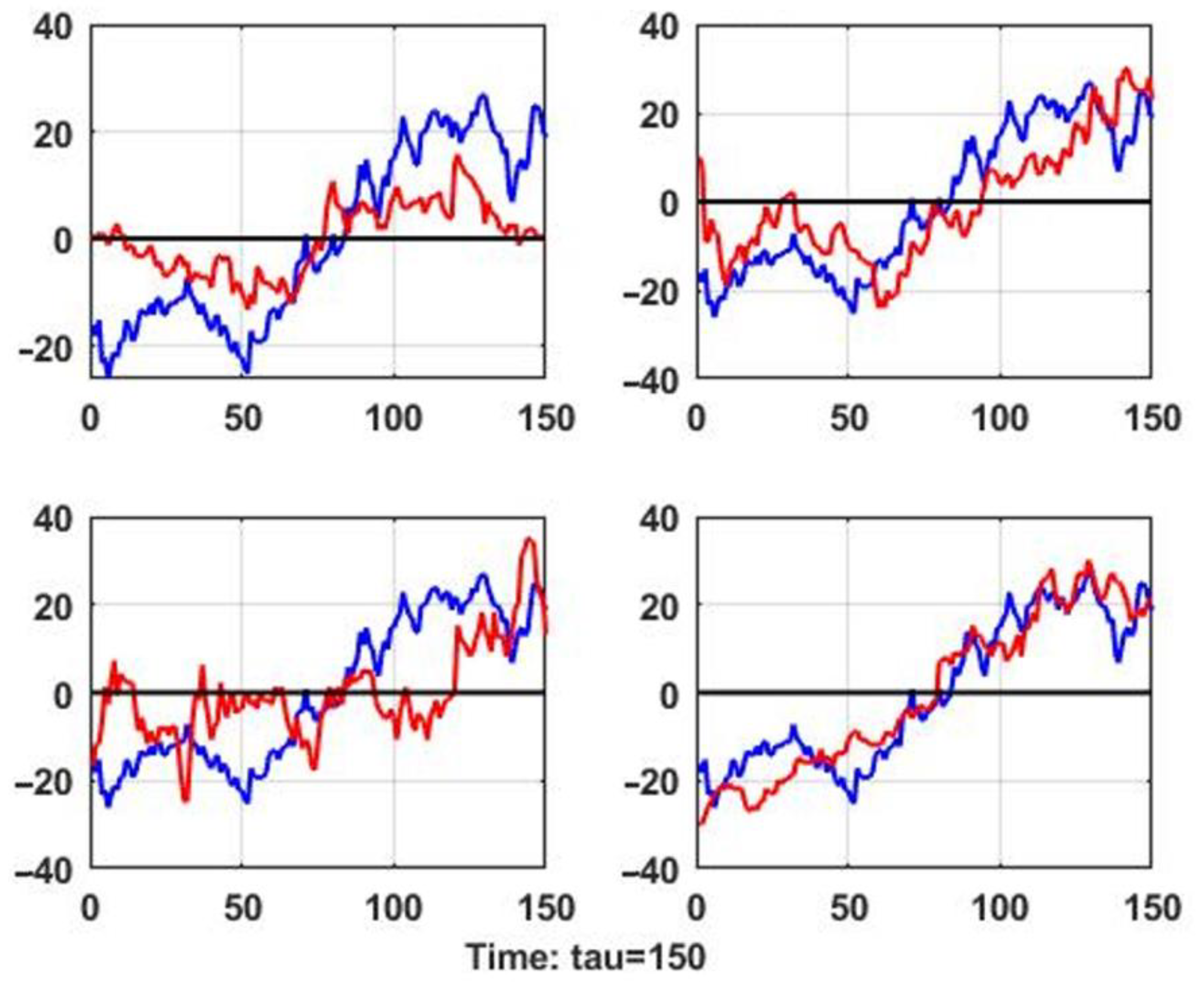
Figure 2 shows the results of the program based on the above algorithm in terms of identifying the situations of analogs.
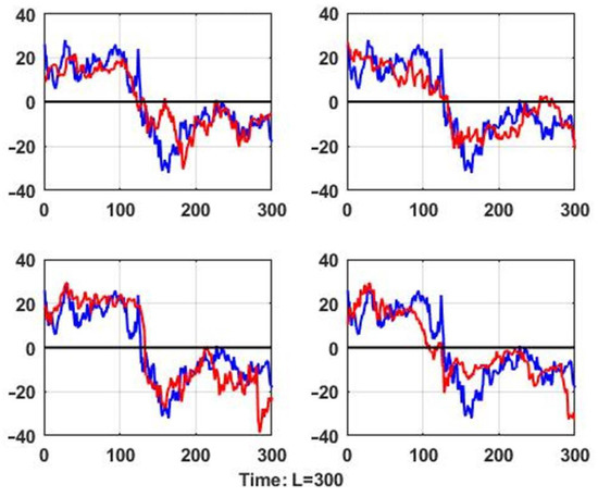
Figure 2.
Analog situations with the shortest distance to the current situation.
In all four diagrams of Figure 2, the same process corresponding to the real situation and the four analog situations with the lowest values of similarity metrics identified during the process of scanning the retrospective database are presented.
Figure 3 shows the aftereffects corresponding to the analogs found, which are used as predictions. For comparisons of their efficiency, the same graphs show the dynamics of the real process in the prediction section.
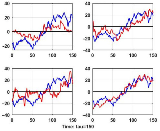
Figure 3.
Effects of analogous situations used as a prediction and their relationship to the actual predicted process.
Figure 3 shows the previously mentioned feature of chaotic dynamics, which does not provide a simple linear conclusion that the degree of similarity of the situation–indicator unambiguously corresponds to the degree of similarity of the aftereffect. In particular, it can be shown that the prediction corresponding to the precedent situation and corresponding to the minimum value of the chosen similarity metric is not the best one.
It should be noted that the similarity of the aftereffects for similar situations is not guaranteed for stationary random processes either, but on average this requirement will be fulfilled. The prediction improvement of chaotic processes by averaging aftereffects is not guaranteed and requires additional research.
Nevertheless, the above example shows possibility of application of the precedent analysis for the problem of chaotic process forecasting. The improvement of this approach on the basis of certain methods of structural and parametric adaptation of the model used to form the prediction algorithm is to be discussed.
3.2. Preliminary Numerical Studies and Results
First, it is necessary to verify the validity of the precedent analysis in the problem of chaotic dynamics prediction. It is necessary to confirm the deterioration of the prediction accuracy with the increase in the number of the reference window. Otherwise, if the accuracy turns out to be unchanged on average, it will mean that the consequence cannot be used as a forecast.
The average value of the mean square error of the forecast is used as an estimate of the quality of the forecast:
Calculations of CVO were performed for two metrics, (4) and (5), used in the process of search for window analogs. Averaging was carried out for N = 100 realizations.
Table 1 shows the growth of the CVO prediction (10) by increasing number of the analog window, i.e., when its degree of similarity to the current situation decreases. It is not possible to obtain a uniformly increasing sequence under unstable dynamics of the observed process. Nevertheless, the obtained result allows us to conclude that it is possible to apply the precedent analysis for the class of observational series.

Table 1.
Average values of the centered values of observations (CVO) prediction for window analogs.
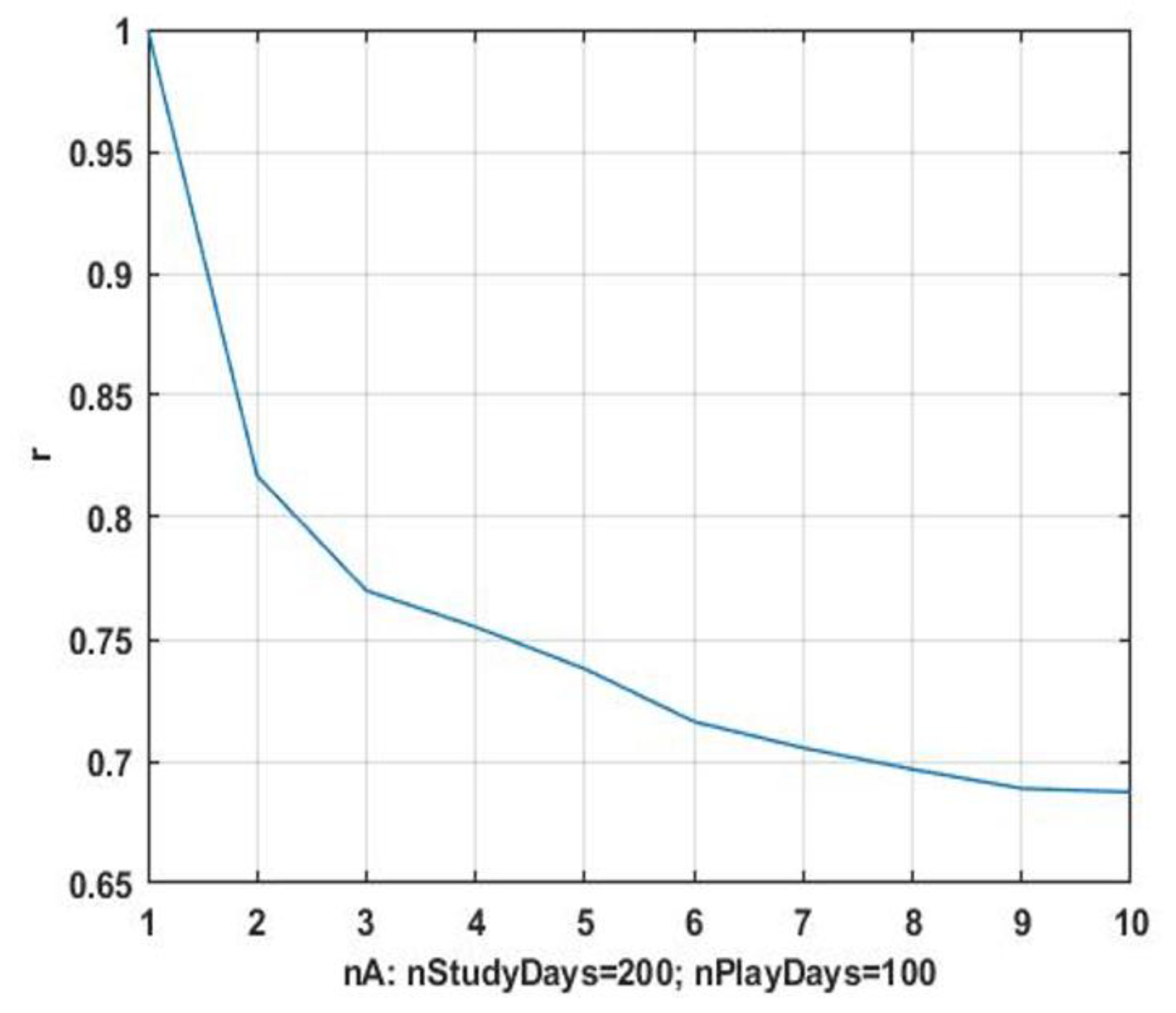
It is necessary to search for windows in order to obtain a uniformly increasing sequence. A search for window-analogs of the current situation is performed for this purpose, the consequences of which are used as a preliminary estimate of the forecast. The final prediction is made by piecewise averaging of the preliminary estimates. The gain in accuracy as compared to the prediction using the precedent aftereffects is estimated as a relative reduction of the prediction error. The corresponding result for = 1, 2, …, 10 window-analogs is shown in Figure 4. It shows that the proposed computational scheme makes it possible to significantly increase the prediction accuracy.
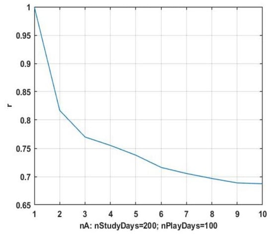
Figure 4.
Dependence of the increase in relative accuracy from the number of analog windows.
One of the important questions without an explicit answer for chaotic dynamics problems is the determination of the best scanning window size L. Obviously, an increase in the window size leads to an increase in the dynamical error due to poorly predictable and rapid changes in the chaotic system component of the observed process, while its reduction leads to a substantial increase in the influence of the random component in the model (1). The methodology for determining the optimal size L by minimizing the total square of the error used in such cases is also not viable due to the essential non-stationarity of the observed process. The approach for selection of the scanning window size based on numerical studies of large observational arrays is considered.
The problem of estimation the prediction quality for different observation sites and different values of the value L is to be discussed.
In this study, it is not the absolute prediction accuracy which is important, but the relative value that characterizes the change in the prediction quality depending on the growth of the state and scanning windows size. In this regard, only the precedent, i.e., the window with the highest degree of similarity to the current situation, will be used as a prototype.
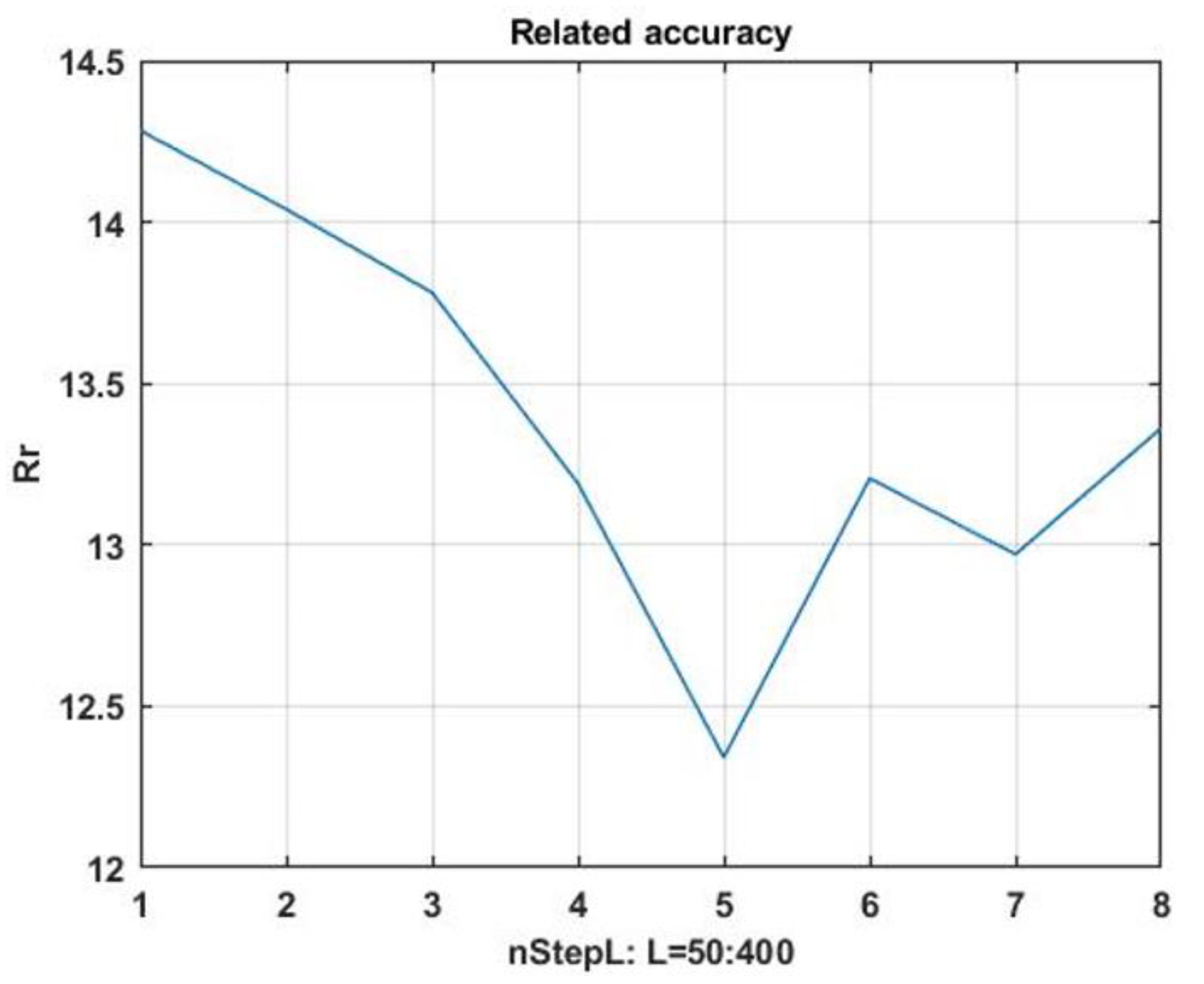
The range of variation of the counts is considered. As an indicator of forecast quality, as in the previous case, the average value of cumulative forecast errors in 100–150 steps of the forecast is used. The results of the program to estimate the dependence of the forecast quality on the size of the scanning window are shown in Figure 5. The best value of the scanning window size lies in the range of change in the counts . However, due to the non-stationarity of the observed process, the best value is not a constant and, therefore, it is advisable to include this value in the list of refined parameters for the adaptive computational scheme.

Figure 5.
Dependence of the prediction quality index on the size of the scanning window.
Another important aspect to be investigated the determination of the feasibility and parameters of the preliminary smoothing of the observational series. According to the previously used computational scheme, search for window analogs was carried out by direct unsmoothed measurements. Unsmoothed measurements were used as prediction, which does not correspond to the traditional concept of prediction, which implies restoration of the system component of the model (1). In this connection, it is expedient to implement the whole process of the precedent prediction on smoothed data, formed by one or another method of dynamic filtering. Then, the search process in the retrospective data will be focused on the system component of the process, which should increase the reliability of intermediate decisions on the choice of the situations-analogs.
In this work, the simplest exponential smoothing was used
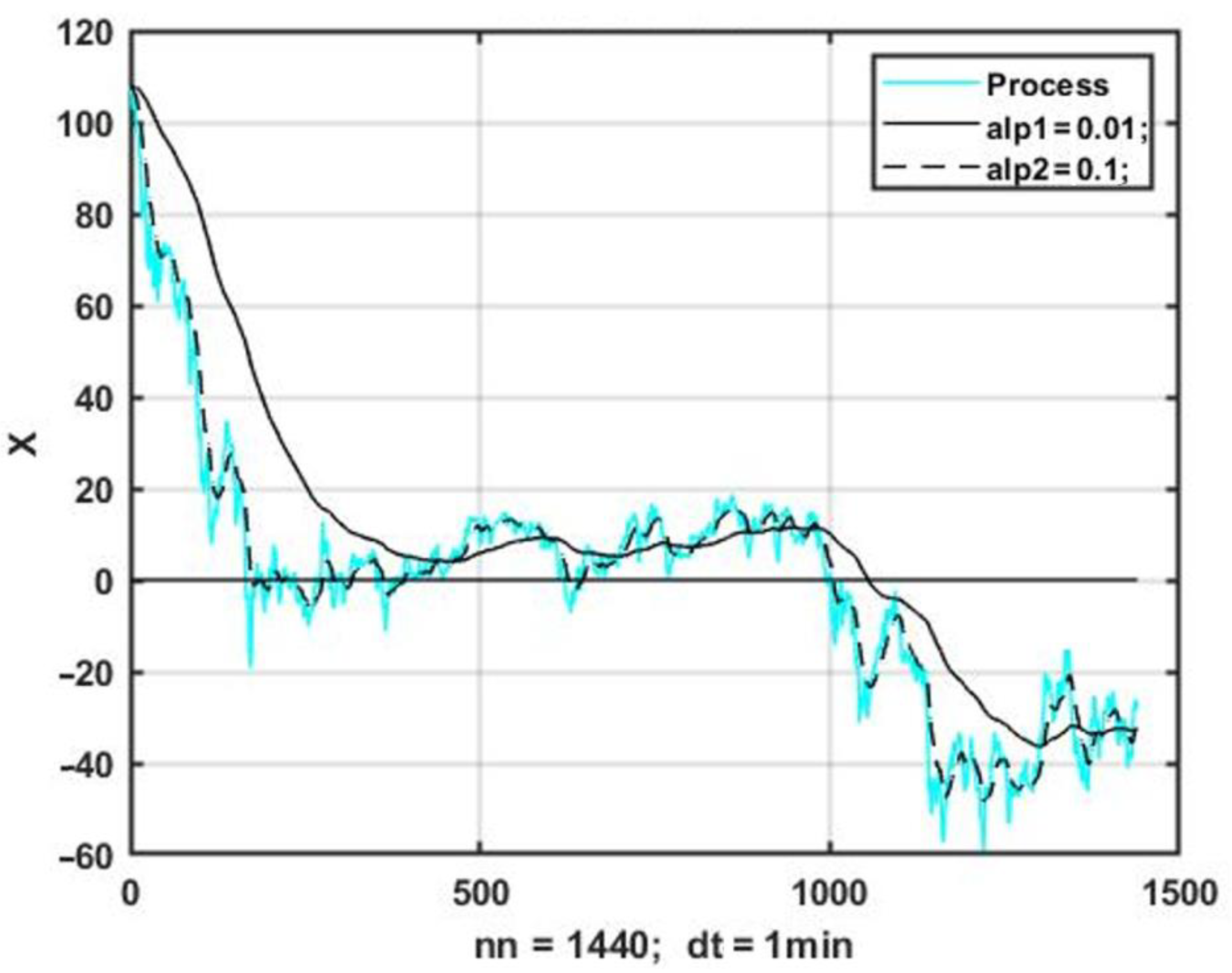
with a smoothing coefficient = 0.01–0.3. The main problem of sequential smoothing is that it leads to estimation bias caused by a dynamic delay of the smoothed process relative to the initial series of observations. Increasing the filter transfer coefficient leads to decreasing the dynamic bias, but at the same time the degree of smoothing of the observation series decreases. The latter statement is illustrated in Figure 6 for two values of the filter coefficient and .
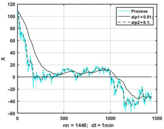
Figure 6.
Exponential smoothing at different filter coefficients.
In this case, it is important to know the changes in the quality of the precedent prediction when switching to smoothed observational series. To this end, the problem of prediction quality estimation is solved again, provided that the search for precedent and counterpart situations is performed on the basis of the similarity analysis of smoothed versions of the observed process. Exponential smoothing (11) was performed for transfer coefficients with values of = 0.01, 0.025, 0.05, 0.1, 0.25, 0.5, 0.75, and 1.0. The degree of smoothness of the process is an inverse value to the value of the filter gain.
The dependence of the average prediction slope (10) from the value of the exponential filter gain is shown in Figure 7. The average estimate of the CVO for the non-smoothed process (dashed line), with changes of a non-systemic nature caused by the non-stationary nature of the observation series is shown.
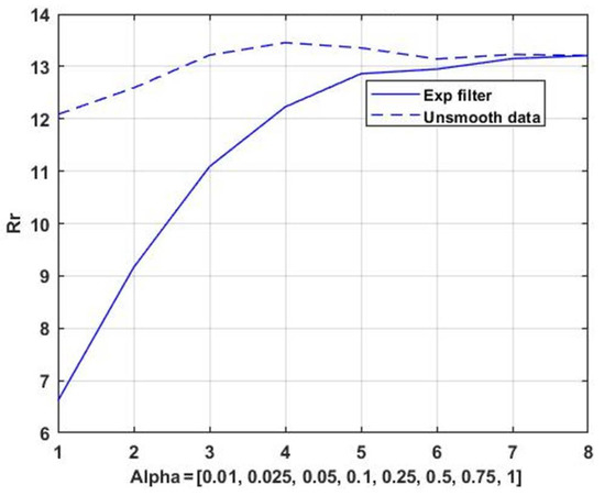
Figure 7.
Dependence of the average value CVO of the precedent prediction score on the value of the filtering coefficients.
The accuracy of the precedent prediction can be significantly improved by filtering the noise of the observations. Nevertheless, the degree of smoothing of the observations is limited by the growth of the bias. In the general case, the filter transfer coefficient , as well as other optional parameters, is advisable to be included in the list of parameters subject to parametric optimization.
3.3. Evolutionary Modeling Method Applied to the Problem of Dynamic Adaptation of the Precedent Prediction Algorithm
The technology of evolutionary modeling proposed in [16] and developed in a large number of studies in the field of data analysis [17,18,19,20] is based on the simulation of the Darwinian self-developing process of evolution of biological populations using the principles of variability and selection.
The possibility of algorithmic realization of these principles as applied to the problem under consideration to be considered.
The principle of variability is based on the emergence of relatively small random changes in model parameters during the formation of a set of descendants of i-th generation from a set of ancestors models. In formalized formulation it is a question of formation and application of i-th generation models’ variability and reproduction operator,
where is the number of ancestor models, is the number of descendant models in each generation, and is the coefficient of multiplication of ancestor models.
Combination of sets of ancestor and descendant models forms new generation of models , subjected to testing, selection, and selection. The number of changes of generations is set beforehand, or determined from the condition of stopping the growth of the efficiency index of the problem to be solved.
The number of modifiable parameter, the type, and value of the modifiable parameter are determined by casting a random variable according to the scheme adopted in the Monte Carlo method.
Three methods of modifying the selected parameter are applied:
1. Natural variability. This type of variability is the most common, occurs with probability , and represents relatively small random fluctuations in model parameters. Natural variability is usually formed as a random variable subject to the normal law , where is the value of k-th parameter in i-th model, is the value of the same parameter in the previous generation of models, is estimate of the standard deviation (RR) of possible variations .
2. Parametric mutation. It differs from natural variability by low probability of occurrence and high values of a changeable parameter. It is estimated by drawing a random variable .
3. Nonparametric mutation. Characterized by unlikely changes in model structure. In the simplest case, it can consist of a change in the order or dimension of the model.
The problem of variability can be solved in different ways. In nature, in most cases formation of progeny genome is performed by combining genes from genomes of different sex parents. Selection of offspring parameters is performed by random selection of parameters from one or another parent. This approach is used when genetic algorithms of sequential optimization are used.
The principle of selection and selection consists in the sequential selection of the best models for a new generation of parent models. The selection process is carried out on the basis of the selected performance indicator of the selected model . Values of similarity metrics (4)–(6) can serve as intermediate performance indicators. However, if the metrics themselves are attributed to the number of modifiable parameters, it is obviously incorrect to compare the degree of similarity on the basis of different metrics. In this connection, it is reasonable to choose as the terminal performance indicator an estimate of prediction accuracy based on the chosen variant of the model.
The selection and selection operator for the i-th generation of models can be represented as
where is number of “surviving” models, which are allowed for further reproduction-modification; is number of strategies of one generation.
If is a particular variant of a predictive model given with given structure and parameters , and accepted as a base “parent model”, then the technology of evolutionary optimization is reduced to the cyclic repetition of the sequence of operators (12) and (13):
As selection is performed by the criterion of superiority, strict optimality of the terminal solution is not guaranteed. However, the found solution will be the best one out of the whole set of the random search formed in the process of implementation of the evolutionary technology.
3.4. Numerical Studies of Evolutionary Adaptation of the Precedent Data Analysis Algorithm
Implementation of the precedent prediction algorithm described above was supplemented by an adaptation contour implemented on the basis of the evolutionary modeling method. The adaptation was reduced to the cyclic alternation (14) of the operators of variability (14), and selection and selection (13).
Varying type was performed with a probability of 0.9 for small natural variability, 0.05 for parametric mutation, and 0.05 for structural mutation. The vector of parameters acted as genome, where is the scan window size, is the scan step value, is exponential filter transfer coefficient (11), is the number of analog windows used in prediction formation, and is the number of similarity metric used. The first three parameters of genome were subjected to natural variability in variation ranges = [50, 400], = [25, 200], and parametric mutation, at which the given variation ranges were tripled. Nonparametric mutation was carried out for parameters , changing in the integer range of 1 to 6 and , with an integer range of variation of 1 to 3. As metrics the relations (4) and (5) and the quadratic metric with normalization of scanning windows and the state of the estimation of the number of observations in these windows were used:
where std is the operator for calculating CVO.
The value of the model reproduction coefficient was chosen from the range , the number of surviving models in each generation . The given ranges were chosen for empirical considerations, and their further increase does not improve convergence of estimation, but leads to a significant increase in the running time of the program.
As an example, Figure 8 shows the convergence of forecast quality index when solving the precedent prediction problem using evolutionary adaptation of prediction models.
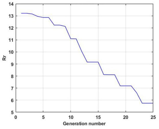
Figure 8.
Dependence of the average value CVO of the precedent prediction score from the model generation number.
From the above graph, we can conclude that it is possible in principle to significantly improve the accuracy when solving the problem of predicting chaotic processes due to the evolutionary adaptation technology considered in the paper.
It is important to note that the result obtained refers only to a specific realization of a chaotic process; an attempt to transfer the found values of the model parameters to another prediction section almost always leads to a substantial decrease in the accuracy of the predictive estimates. In addition, when assessing the accuracy of the generated result, it essentially depends on the substantive formulation of the problem for the benefit of which the prediction is carried out. A relative increase in the prediction accuracy does not yet mean its sufficiency, for example, for effectively solving the problem of proactive control of the technological process.
3.5. Specific Features of Evolutionary Adaptation of the Precedent Analysis Algorithm for Chaotic Processes
Numerous applications of evolutionary modeling and related genetic algorithms [16,17,18,19,20] enable us to find effective solutions for nonstationary processes with inertia or other stabilizing factors. With respect to turbulent gas-dynamic flows, with low degree of inertia and connectivity, the chaotic component is dominant and high accuracy of extrapolation prediction should not be expected.
A preliminary evaluation of the precedent prediction has shown the possibility in principle of such an approach, but in a chaotic environment, the degree of similarity of the precedent does not guarantee the similarity of the found consequence to the predicted situation. In this regard, unlike the traditional approach based on the nearest-neighbor method, the task consists in finding analogous situations, relying not only on the degree of its similarity according to the chosen proximity criterion, but, above all, on choosing such a model, which would provide the greatest terminal efficiency, evaluated through prediction accuracy.
An alternative solution to the proposed option consists in the a priori formation of a pool of prognostic algorithms, including sets of solving rules, lists of modifiable parameters, and their critical values and ranges of variation. The advantage of this approach is the convenience of its implementation. However, it limits the number of freedom degrees of machine choice; there is no possibility to obtain radically new, unexpected solutions, not foreseen by a programmer or a system analyst. It is clear that with any regularization, any additional set of constraints can close access to unexpected original solutions.
At the same time, the complete removal of constraints in the random formation of predictive algorithms will lead to an infinite number of meaningless computational schemes. Waiting for any sensible solution to emerge would require a time commensurate with real biological evolution.
Evolutionary technology, like the whole probabilistic-statistical paradigm, is implicitly oriented toward the comfortable hypothesis of repeatable experiments under unchanging or slowly changing conditions. The transition to non-stationary, and even more chaotic processes, inevitably destroys the statistical basis of predictive technology. To some extent, this also applies to evolutionary modeling. However, in the nature of chaos, as a rule, there are some regularizing effects that reduce the degree of total uncertainty. If evolutionary technology can isolate, at least not explicitly, and use such latent regularities, the task of building effective predictive technologies may be feasible.
In addition, the application of the evolutionary computational scheme will make it possible to answer the question about the fundamental admissibility of one or another class of predictive technologies.
3.6. Analysis of the Dynamic and Statistical Characteristics of an Unstable Gas-Dynamic System
The series of observations were obtained during the monitoring of the technological process (TP) which takes place in an unstable gas-dynamic environment. In this case, the instability of the medium is defined as the chaotic nature of the dynamic process which describes the unsymmetrical changes in the phase state parameters (or state vector) of the simulated object. The data used are centered and normalized deviations of measured physical parameters from their values defined by technological regulations of the TP.
As a system component a posteriori conditional mean, obtained on the basis of one of the known algorithms of statistical smoothing, was used; in particular, polynomials of a given order with parameter fitting using the least squares method (LQM).
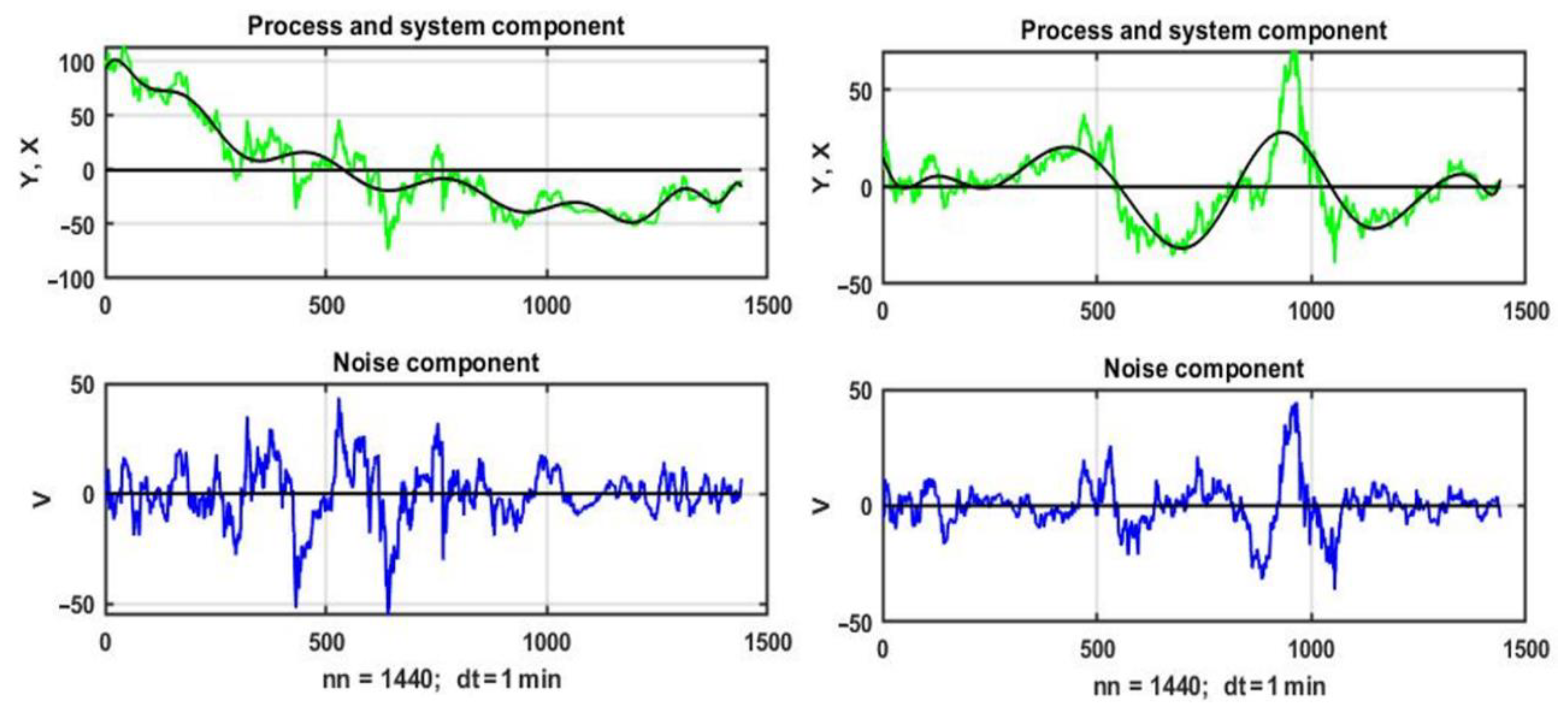
Plots of the system component X(t) of the observation model (1), obtained by MNA fitting of the corresponding noisy curves (upper figures), and plots of the noise component V(t) (lower figures) are presented in Figure 9. In both cases, a polynomial approximation of the 15th degree was used to extract the system component. At the same time, generalized inverse was used in solving the system of normal equations, as the use of approximating polynomials of degree 4 and higher led to degeneracy of the observation matrix.
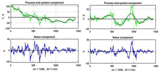
Figure 9.
System and noise components in observations of parameter states of an unstable environment.
An alternative approach to extract the system component is related to the application of spline approximation. The selection of spline approximation nodes was performed manually at points close to local extrema and inflection points. An example of the formation of a reference curve for a one-day monitoring interval is shown in Figure 10.
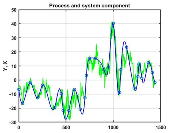
Figure 10.
System component of a process based on cubic spline approximation (green—experimental data a one-day monitoring, blue—spline approximation).
The graphs show an oscillating, non-periodic, unsymmetrical process with multiple local trends which do not passes for explicit extrapolation computational schemes. If desired, this observation can be confirmed formally by using the eigenvalues of the linearization matrix in the neighborhood of the stationary point. In the general case, Lyapunov characteristic indices are used to study the behavior in the neighborhood of a random trajectory [25]. The Lyapunov exponents serve as a measure of chaotic behavior: if there are positive exponents, then the behavior of the dynamical system is chaotic.
Statistical analysis of the noise component was carried out based on known methods for testing statistical hypotheses [26,27]. The stationarity of the noise component was checked using the ascending and descending series criterion and the Abbe criterion. The stationarity hypothesis was rejected at the 0.95 confidence level. Pearson’s criterion was used for normality checking. Analysis of the Gaussianity of the observations showed a slow convergence to a normal distribution. The main difference is in the weighting of the distribution tips, indicating the presence of anomalous observations.
4. Conclusions
Numerous applications of evolutionary modeling presented in the article allow the drawing of conclusions about the possibility of predicting the state of dynamic systems in unsymmetrical, unstable environments, whose dynamics are described by chaotic processes, based on technology of precedent data analysis. In this case, an increase in the accuracy of prediction can be achieved by means of the computational scheme of dynamic adaptation, based on the well-known method of evolutionary modeling.
In this case, the inertia, which is typical of any physical process, serves as an implicit regulating factor which allows one to reveal the local ordering in a chaotic process. By transition to inertia-free environments, such as the dynamics of quotations of currency instruments in the Forex market, the result is less effective.
The presence of “vertical” correlations in series of multidimensional chaotic processes and “horizontal” autocorrelations allowing dynamically optimizing the size of the scanning window should be considered as alternative regularizing factors.
Author Contributions
Conceptualization, methodology, validation, and writing, A.M.; review and editing, investigation, visualization, supervision, and funding acquisition, E.B. Both authors have read and agreed to the published version of the manuscript.
Funding
This study was supported by the grants of Russian Fundamental Research Fund (№ 17-29-07073, 18-07-01272, 18-08-01505, 19-08-00989, 20-08-01046) in St. Peters-burg Institute for Informatics and Automation of the Russian Academy of Sciences.
Institutional Review Board Statement
Not applicable.
Informed Consent Statement
Not applicable.
Data Availability Statement
Data is contained within the article.
Acknowledgments
The authors acknowledge support by the Open Access Publication Funds of the TU Dresden.
Conflicts of Interest
The authors declare no conflict of interest.
References
- Broer, H.; Takens, F. Dynamical Systems and Chaos; Springer: Basel, Switzerland; Groningen, The Netherlands, 2009; ISBN 978-3-0348-7520-2. [Google Scholar]
- Smith, L. Chaos: A Very Short Introduction; Oxford University Press: Oxford, UK, 2007; ISBN 978-0-1928-5378-3. [Google Scholar]
- Manneville, P. Instabilities, Chaos and Turbulence: An Introduction to Nonlinear Dynamics and Complex Systems; World Scientific Publishing Company: Singapore, 2004; ISBN 978-1-8609-4491-8. [Google Scholar]
- Lorenz, E. The Essence of Chaos; University of Washington: Washington, DC, USA, 1996; ISBN 02959751-48. [Google Scholar]
- Kautz, R. Chaos: The Science of Predictable Random Motion; Oxford University Press: Oxford, UK, 2011; ISBN 978-0-19-959458-0. [Google Scholar]
- Klimontovich, Y.L. Turbulent Motion and the Structure of Chaos. A New Approach to the Statistical Theory of Open Systems, 2nd ed.; URSS Publ.: Moscow, Russia, 2010; ISBN 978-5-4840-1197-1. [Google Scholar]
- Musaev, A.; Borovinskaya, E. Prediction in Chaotic Environments Based on Weak Quadratic Classifiers. Symmetry 2020, 12, 1630. [Google Scholar] [CrossRef]
- Abbasifard, M.R.; Ghahremani, B.; Naderi, B.H. A Survey on Nearest Neighbor Search Methods. Int. J. Comput. Appl. 2014, 95, 39–52. [Google Scholar]
- Dhanabal, S.; Chandramathi, S. A Review of various k-Nearest Neighbor Query Processing Techniques. Int. J. Comput. Appl. 2011, 7, 7–22. [Google Scholar]
- Mahapatra, R.P.; Chakraborty, P.S. Comparative Analysis of Nearest Neighbor Query Processing Techniques. Procedia Comput. Sci. 2015, 57, 1289–1298. [Google Scholar] [CrossRef][Green Version]
- Advances in Data Mining. Applications and Theoretical Aspects. Proceedings. Lecture Notes in Computer Science; Springer: Berlin/Heidelberg, Germany, 2018; p. 10933. ISBN 978-3-319-95785-2.
- Larose, D.; Larose, C. Discovering Knowledge in Data, 2nd ed.; Wiley: New York, NY, USA, 2014; ISBN 978-0-470-90874-7. [Google Scholar]
- Fukunaga, K. Introduction to Statistical Pattern Recognition, 2nd ed.; Academic Press: Cambridge, MA, USA, 2013; ISBN 0-12-269851-7. [Google Scholar]
- Bishop, C. Pattern Recognition and Machine Learning; Springer: New York, NY, USA, 2006; ISBN 978-0-387-31073-2. [Google Scholar]
- Hastie, T.; Tibshirani, R.; Friedman, J. The Elements of Statistical Learning, 2nd ed.; Springer Series in Statistics; Springer: Berlin/Heidelberg, Germany, 2017; ISBN 978-0-387-84857-0. [Google Scholar]
- Fogel, L.J.; Owens, A.J.; Walsh, M.J. Artificial Intelligence through Simulated Evolution; John Wiley & Sons: New York, NY, USA, 1966; ISBN 978-0-471-26516-0. [Google Scholar]
- Carreno, J.E. Multi-objective optimization by using evolutionary algorithms: The p-Optimality Criteria. IEEE Trans. Evol. Comput. 2014, 18, 167–179. [Google Scholar]
- Das, S.; Suganthan, P.N. Differential Evolution: A Survey of the State-of-the-Art. IEEE Trans. Evol. Comput. 2011, 15, 4–31. [Google Scholar] [CrossRef]
- Mukhopadhyay, A.; Maulik, U.; Bandyopadhyay, S.; Coello, C.A. A Survey of Multiobjective Evolutionary Algorithms for Data Mining: Part I. IEEE Trans. Evol. Comput. 2014, 18, 4–19. [Google Scholar] [CrossRef]
- Musaev, A.A. Evolutionary-statistical approach to self-organization of predictive models of technological process control. Autom. Ind. 2006, 7, 31–35. [Google Scholar]
- Sinai, Y.G. Probability Theory: An Introductory Course; Springer: Berlin/Heidelberg, Germany, 2020; ISBN 978-3540533481. [Google Scholar]
- Meyer, M.C. Probability and Mathematical Statistics: Theory, Applications, and Practice in R; SIAM: Philadelphia, PA, USA, 2019; ISBN 978-1-611-97577-2. [Google Scholar]
- Maronna, R.; Martin, R.; Yohai, V.; Salibián-Barrera, M. Robust Statistics: Theory and Methods (with R), 2nd ed.; Wiley: New York, NY, USA, 2018; ISBN 978-1-119-21468-7. [Google Scholar]
- Launer, R.; Wilkinson, G. Robustness in Statistics; Academic Press: Cambridge, MA, USA, 1979; ISBN 978-0-12-438150-6. [Google Scholar]
- Loskutov, A. Mathematical foundations of chaotic dynamical systems. Successes Phys. Sci. 2007, 177, 989–1015. [Google Scholar]
- Lehmann, E.L.; Romano, E.J. Testing Statistical Hypotheses, 3rd ed.; Springer: Berlin/Heidelberg, Germany, 2005; ISBN 0-387-98864-5. [Google Scholar]
- Ayvazyan, S.; Mkhitaryan, V. Applied Statistics and Fundamentals of Econometrics; Unity: Moscow, Russia, 1998; ISBN 5-238-00013-8. [Google Scholar]
Publisher’s Note: MDPI stays neutral with regard to jurisdictional claims in published maps and institutional affiliations. |
© 2021 by the authors. Licensee MDPI, Basel, Switzerland. This article is an open access article distributed under the terms and conditions of the Creative Commons Attribution (CC BY) license (http://creativecommons.org/licenses/by/4.0/).


