New Self-Adaptive Inertial-like Proximal Point Methods for the Split Common Null Point Problem

Abstract

Symmetry plays an important role in solving practical problems of applied science, especially in algorithm innovation. In this paper, we propose what we call the self-adaptive inertial-like proximal point algorithms for solving the split common null point problem, which use a new inertial structure to avoid the traditional convergence condition in general inertial methods and avoid computing the norm of the difference between $x_n$ and $x_{n-1}$ before choosing the inertial parameter. In addition, the selection of the step-sizes in the inertial-like proximal point algorithms does not need prior knowledge of operator norms. Numerical experiments are presented to illustrate the performance of the algorithms. The proposed algorithms provide enlightenment for the further development of applied science in order to dig deep into symmetry under the background of technological innovation.

1. Introduction

We are concerned with the following split common null point problem (SCNPP):

$$\begin{array}{cc}\hfill & \mathrm{find}{x}^{\ast }\in H_1\mathrm{to} \mathrm{solve}0\in A\left(x^{\ast }\right)\hfill \\ \hfill & \mathrm{and}\hfill \end{array}$$

(1)

$$\begin{array}{cc}\hfill & y^{\ast } = T{x}^{\ast }\in H_2\mathrm{to} \mathrm{solve}0\in B\left(y^{\ast }\right),\hfill \end{array}$$

(2)

where $H_1$ and $H_2$ are Hilbert spaces, $A:H_1\to 2^{H_1}$ and $B:H_2\to 2^{H_2}$ are set-valued mappings, and $T:H_1\to H_2$ is a nonzero bounded linear operator.

The SCNPP (1) and (2), which covers the convex feasibility problem (CFP) (Censor and Elfving [1]), variational inequalities (VIs) ( Moudafi [2]), and many constrained optimization problems as special cases, has attracted important attention both theoretically and practically (see Byrne [3], Moudafi and Thukur [4]).

The main idea to solve SCNPP comes from symmetry, that is, invariance. Therefore, fixed point theory plays a key role here. We recall the resolvent operator $J_r^A = {(I+rA)}^{-1}, r > 0$, which plays an essential role in the approximation theory for zero points of maximal monotone operators as well as in solving (1) and (2) and has the following key facts.

Fact 1: 

The resolvent is not only always single-valued but also firmly monotone:

$$\begin{array}{c}\hfill ⟨J_r^{A}x-J_r^{A}y,x-y⟩ \ge {\parallel J_r^{A}x-J_r^{A}y\parallel }^2.\end{array}$$

(3)

Fact 2: 

Using the resolvent operator, the problem (1) and (2) can be written as a fixed point problem:

$$\begin{array}{c}\hfill x^{\ast } = J_{\lambda }^A(I-\gamma T^{\ast }(I-J_{\lambda }^B)T)x^{\ast }, \lambda > 0, \gamma > 0.\end{array}$$

Fact 2 transforms the problem (1) and (2) into a fixed-point problem, and the research of the latter reflects the invariance in transformation, which is the essence of symmetry. Based on Fact 2, Byrne, et al. [5] proposed the following forward–backward algorithm:

$$\begin{array}{c}\hfill x_{n+1} = J_{\lambda }^A(x_n-\gamma T^{\ast }(I-J_{\lambda }^B)T{x}_n)\end{array}$$

(4)

and obtained weak convergence, where $T^{\ast }$ is the adjoint of T, the stepsize $\gamma \in (0,\frac{2}{L})$ with $L = \parallel T^{\ast }T\parallel$.

At the same time, the inertial method originating from the heavy ball with friction system has attracted increasing attention thanks to its convergence properties in the field of continuous optimization. Therefore, many scholars have combined the forward–backward method (4) with the inertial algorithm to study the SCNPP and proposed some iterates. For related works, one can consult Alvarez and Attouch [6], Alvarez [7], Attouch et al. [8,9,10], Akgül [11], Hasan et al. [12], Khdhr et al. [13], Ochs et al. [14,15], Dang et al. [16], Soleymani and Akgül [17], Suantai et al. [18,19], Dong et al. [20], Sitthithakerngkiet et al. [21], Kazmi and Rizvi [22], Promluang and Kumman [23], Eslamian et al. [24], and references therein.

Although these algorithms improved the numerical solution of the split common null point problem, there exist two common drawbacks: one is that the step size depends on the norm of the linear operator T, which means there is a high computation cost, because the norm of the linear operator must be estimated before selecting the step size; another drawback is that the following condition is required:

$$\begin{array}{c}\hfill \sum _{n=1}^{\infty }{\alpha }_n{\parallel x_n-x_{n-1}\parallel }^2 < \infty ,\end{array}$$

(5)

which means that one not only needs to calculate the norm of the difference between $x_n$ and $x_{n-1}$ in advance at each step but also check if ${\alpha }_n$ satisfies (5).

So it is natural to ask the following questions:

Question 1.1 

Can we construct the iterate for SCNPP whose step size does not depend on the norm of the linear operator T?

Question 1.2 

Can condition (5) be removed from the inertial method and still ensure the convergence of the sequence? Namely, can we construct a new inertial algorithm to solve SCNPP (1) and (2) without prior computation of the norm of the difference between $x_n$ and $x_{n-1}$?

The purpose of this paper is to present a new self-adaptive inertial-like technique to give an affirmative answer to the above questions. Importantly, the innovative algorithms provide an idea of how to use symmetry to solve real-world problems in applied science.

2. Preliminaries

Let $⟨·,·⟩$ and $\parallel ·\parallel$ be the inner product and the induced norm in a Hilbert space $H$, respectively. For a sequence $\left\{x_n\right\}$ in $H$, denote $x_n\to x$ and $x_n\rightharpoonup x$ by the strong and weak convergence to x of $\left\{x_n\right\}$, respectively. Moreover, the symbol ${\omega }_w\left(x_n\right)$ represents the $\omega$-weak limit set of $\left\{x_n\right\}$, that is,

$$\begin{array}{c}\hfill {\omega }_w\left(x_n\right):=\{x\in H:x_{n_j}\rightharpoonup x\mathrm{for}\mathrm{some}\mathrm{subsequence}\left\{x_{n_j}\right\}\mathrm{of}\left\{x_n\right\}\}.\end{array}$$

The identity below is useful:

$$\begin{array}{cc}\hfill {\parallel \alpha x+\beta y+\gamma z\parallel }^2 =& \alpha {\parallel x\parallel }^2 + \beta {\parallel y\parallel }^2 + \gamma {\parallel z\parallel }^2\hfill \\ \hfill & -\alpha \beta {\parallel x-y\parallel }^2{ - \beta \gamma \parallel y-z\parallel }^2 - \gamma \alpha {\parallel x-z\parallel }^2\hfill \end{array}$$

(6)

for all $x,y,z\in \mathbb{R}$ and $\alpha + \beta + \gamma = 1$.

Definition 1.

A multivalued mapping $A:H\to 2^H$ with domain $D\left(A\right) = \{x\in H,Ax\ne \varnothing \}$ is monotone if

$$\begin{array}{c}\hfill ⟨x-y,x^{\ast }-y^{\ast }⟩ \ge 0,\end{array}$$

(7)

for all $x,y\in D\left(A\right)$, $x^{\ast }\in A\left(x\right)$, and $y^{\ast }\in A\left(y\right)$. A monotone operator A is referred to be maximal if its graph is not properly contained in the graph of any other monotone operator.

Definition 2.

Let H be a real Hilbert space and let $h:H\to H$ be a mapping.

(i) 

h is called Lipschitz with constant $\kappa > 0$ if $\parallel h\left(x\right)-h\left(y\right)\parallel \le \kappa \parallel x-y\parallel$ for all $x,y\in H$.

(ii) 

h is called nonexpansive if $\parallel h\left(x\right)-h\left(y\right)\parallel \le \parallel x-y\parallel$ for all $x,y\in H$.

From Fact 1, we can conclude that $J_r^A$ is a nonexpansive operator if A is a maximal monotone mapping. Moreover, due to the work of Aoyama et al. [25], we have the following property:

$$\begin{array}{c}\hfill ⟨J_r^{A}x-y,x-J_r^{A}x⟩ \ge 0, y\in A^{-1}\left(0\right),\end{array}$$

(8)

where $A^{-1}\left(0\right) = \{z\in H:0\in Az\}$.

Definition 3.

Let C be a nonempty closed convex subset of H. We use $P_C$ to denote the projection from H onto C; namely,

$$\begin{array}{c}\hfill P_{C}x = argmin\{\parallel x-y\parallel :y\in C\},x\in H.\end{array}$$

The following significant characterization of the projection $P_C$ should be recalled: given $x\in H$ and $y\in C$,

$$\begin{array}{c}\hfill P_{C}x = z⟺⟨x-z,y-z⟩ \le 0,y\in C.\end{array}$$

(9)

Lemma 1.

(Xu [26], Maingé [27]) Assume that $\left\{a_n\right\}$ is a sequence of nonnegative real numbers such that

$$\begin{array}{c}\hfill a_{n+1} \le (1-{\gamma }_n{a}_n)a_n + {\gamma }_n{\delta }_n + c_n,n \ge 0,\end{array}$$

where $\left\{{\gamma }_n\right\}$ is a sequence in $(0,1)$ and $\left\{{\delta }_n\right\}$ is a sequence in $\mathbb{R}$ such that

(1) 

${\sum }_{n=1}^{\infty }{\gamma }_n = \infty$;

(2) 

${lim\; sup}_{n\to \infty }{sup}_{n\to \infty }{\delta }_n \le 0$ or ${\sum }_{n=1}^{\infty }{\gamma }_n\left|{\delta }_n\right| < \infty$;

(3) 

${\sum }_{n=1}^{\infty }{c}_n < \infty$.

Then ${lim}_{n\to \infty }{a}_n = 0$.

Lemma 2.

(see, e.g., Opial [28]) Let H be a real Hilbert space and $\left\{x_n\right\}$ be a bounded sequence in H. Assume there exists a nonempty subset $S\subset H$ satisfying the properties:

(i)

${lim}_{n\to \infty }\parallel x_n-z\parallel$ exists for every $z\in S$,

(ii)

${\omega }_w\left(x_n\right)\subset S$.

Then, there exists $\overline{x}\in S$ such that $\left\{x_n\right\}$ converges weakly to $\overline{x}$.

Lemma 3.

(Maingé [29]) Let $\left\{{\mathrm{\Gamma }}_n\right\}$ be a sequence of real numbers that does not decrease at the infinity in the sense that there exists a subsequence $\left\{{\mathrm{\Gamma }}_{n_j}\right\}$ of $\left\{{\mathrm{\Gamma }}_n\right\}$ such that ${\mathrm{\Gamma }}_{n_j} < {\mathrm{\Gamma }}_{n_j+1}$ for all $j \ge 0$. Also consider the sequence of integers ${\left\{\sigma \left(n\right)\right\}}_{n\ge n_0}$ defined by

$$\begin{array}{c}\hfill \sigma \left(n\right) = max\{k\le n:{\mathrm{\Gamma }}_k\le {\mathrm{\Gamma }}_{k+1}\}.\end{array}$$

Then, ${\left\{\sigma \left(n\right)\right\}}_{n\ge n_0}$ is a nondecreasing sequence verifying ${lim}_{n\to \infty }\sigma \left(n\right) = \infty$ and, for all $n \ge n_0$,

$$\begin{array}{c}\hfill max\{{\mathrm{\Gamma }}_{\sigma \left(n\right)},{\mathrm{\Gamma }}_n\} \le {\mathrm{\Gamma }}_{\sigma \left(n\right)+1}.\end{array}$$

3. Main Results

3.1. Variant of Discretization

Inspired by the discretization of the second order dynamic system $\frac{d^{2}x}{d{t}^2} + \lambda \left(t\right)\frac{dx}{dt} + Ax = 0$, we consider the following iterative sequence

$$\begin{array}{c}\hfill x_{n+1} - x_{n-1} - {\theta }_n(x_n-x_{n-1}) + {\gamma }_{n}A\left(x_{n+1}\right)\ni 0,\end{array}$$

(10)

where $x_0$, $x_1$ are two arbitrary initial points, and ${\gamma }_n$ is a real nonnegative number. This recursion can be rewritten as

$$\begin{array}{c}\hfill x_{n+1} = J_{{\gamma }_n}^A(x_{n-1}+{\theta }_n(x_n-x_{n-1})),\end{array}$$

which proves that the sequence $\left\{x_n\right\}$ satisfying (10) always exists for any choice of the sequences $\left\{{\gamma }_n\right\}$ and $\left\{{\theta }_n\right\}$, provided that ${\gamma }_n > 0$.

To distinguish from Alvarez and Attouch’s Inertial-Prox algorithm ([6]), we call it inertial-like proximal point algorithm. Combining the inertial-like proximal point algorithm and the forward–backward method, we propose the following self adaptive inertial-like proximal algorithms.

3.2. Some Assumptions

Assumption 1.

Throughout the rest of this paper, we assume that $H_1$ and $H_2$ are Hilbert spaces. We study the split common null point problem (SCNPP) as (1) and (2), where $A:H_1\to 2^{H_1}$ and $B:H_2\to 2^{H_2}$ are set-valued maximal monotone mappings, respectively, and $T:H_1\to H_2$ is a bounded linear operator, $T^{\ast }$ means the adjoint of T.

Assumption 2.

The functions are defined as:

$$\begin{array}{c}\hfill f\left(x\right) = \frac{1}{2}{\parallel (I-J_r^A)x\parallel }^2,F\left(x\right) = (I-J_r^A)x,r > 0;\end{array}$$

and

$$\begin{array}{c}\hfill g\left(x\right) = \frac{1}{2}{\parallel (I-J_{\mu }^B)Tx\parallel }^2,G\left(x\right) = T^{\ast }(I-J_{\mu }^B)Tx,\mu > 0.\end{array}$$

Assumption 3.

Denote by Ω the solution set of the SCNPP (1) and (2); namely,

$$\begin{array}{c}\hfill \mathsf{\Omega } = \left\{x^{\ast }\in H_1:0\in A\left(x^{\ast }\right)\mathrm{and}0\in B\left(T{x}^{\ast }\right)\right\},\end{array}$$

and we always assume $\mathsf{\Omega }\ne \varnothing$.

3.3. Inertial-like Proximal Point Algorithms

Remark 1.

It is not hard to find that if $\parallel F\left(y_n\right){\parallel }^2 + {\parallel G\left(y_n\right)\parallel }^2 = 0$ for some $n \ge 0$, then $x_n$ is a solution of the SCNPP (1) and (2), and the iteration process is terminated in finite iterations. In addition, if ${\theta }_n\equiv 1$ and step size ${\tau }_n$ depends on the norm of linear operator T, Algorithm 1 recovers Byrne et al. [5].

Algorithm 1 Self adaptive inertial-like algorithm

Initialization: Choose a sequence $\left\{{\theta }_n\right\}\subset [0,1]$ satisfying one of the three cases: (I.) ${\theta }_n\in (0,1)$ such that ${{\displaystyle \underline{lim}}}_{n\to \infty }{\theta }_n(1-{\theta }_n) > 0$; (II.) ${\theta }_n\equiv 0$; or (III.) ${\theta }_n\equiv 1$. Select arbitrary initial points $x_0$, $x_1$. Iterative Step: After constructing the nth-iterate $x_n$, compute $$\begin{array}{c}\hfill y_n = x_{n-1} + {\theta }_n(x_n-x_{n-1}),\end{array}$$ (11) and define the $(n+1)$th iterate by $$\begin{array}{c}\hfill x_{n+1} = J_r^A(I-{\tau }_n{T}^{\ast }(I-J_{\mu }^B)T)y_n,\end{array}$$ (12) where ${\tau }_n$ is defined as $$\begin{array}{c}\hfill {\tau }_n = \left\{\begin{array}{cc}\frac{g\left(y_n\right)}{\parallel F\left(y_n\right){\parallel }^2+{\parallel G\left(y_n\right)\parallel }^2},\hfill & \mathrm{if}\parallel F\left(y_n\right){\parallel }^2 + {\parallel G\left(y_n\right)\parallel }^2\ne 0\hfill \\ 0,\hfill & \mathrm{otherwise}.\hfill \end{array}\right.\end{array}$$

Remark 2.

In the subsequent convergence analysis, we will always assume that the two algorithms generate an infinite sequence, namely, the algorithms are not terminated in finite iterations. In addition, in the simulation experiments, we will give a stop criterion to end the iteration for practice.

3.4. Convergence Analysis of Algorithms

Theorem 1.

If the assumptions (A1)–(A3) are satisfied, then the sequence $\left\{x_n\right\}$ generated by Algorithm 1 converges weakly to a point $z\in \mathsf{\Omega }$.

Proof. 

To this end, the following three situations will be discussed: (I). ${\theta }_n\in (0,1)$, ${{\displaystyle \underline{lim}}}_{n\to \infty }{\theta }_n(1-{\theta }_n) > 0$; (II). ${\theta }_n\equiv 0$; and (III). ${\theta }_n\equiv 1$.

(I).

First, we consider the case of ${\theta }_n\in (0,1)$, ${{\displaystyle \underline{lim}}}_{n\to \infty }{\theta }_n(1-{\theta }_n) > 0$.

Without loss of generality, we take $z\in \mathsf{\Omega }$, and then we have $z = J_r^{A}z, Tz = J_{\mu }^{B}Tz$ and $J_r^A(I-{\tau }_n{T}^{\ast }(I-J_{\mu }^B)T)z = z$ from Fact 2. It turns out from (11) and (7) that

$$\begin{array}{ccc}\hfill \parallel y_n{-z\parallel }^2& =& \parallel x_{n-1}+{\theta }_n(x_n-x_{n-1}){-z\parallel }^2\hfill \\ & =& {\theta }_n\parallel x_n{-z\parallel }^2 + (1-{\theta }_n)\parallel x_{n-1}{-z\parallel }^2 - {\theta }_n(1-{\theta }_n){\parallel x_n-x_{n-1}\parallel }^2.\hfill \end{array}$$

(13)

Since $J_r^A$ is nonexpansive, it follows from (12) that

$$\begin{array}{ccc}\hfill \parallel x_{n+1}{-z\parallel }^2& =& \parallel J_r^A(I-{\tau }_n{T}^{\ast }(I-J_{\mu }^B)T)y_n{-z\parallel }^2\hfill \\ & \le & \parallel (I-{\tau }_n{T}^{*}(I-J_{\mu }^B)T)y_n{-z\parallel }^2\hfill \\ & =& \parallel y_n{-z\parallel }^2 - 2{\tau }_n⟨y_n-z,T^{\ast }(I-J_{\mu }^B)T{y}_n⟩ + {\tau }_n^2{\parallel T^{\ast }(I-J_{\mu }^B)T{y}_n\parallel }^2\hfill \\ & =& \parallel y_n{-z\parallel }^2 - 2{\tau }_n⟨T{y}_n-Tz,(I-J_{\mu }^B)T{y}_n⟩ + {\tau }_n^2{\parallel G\left(y_n\right)\parallel }^2.\hfill \end{array}$$

(14)

It follows from the property (8) of resolvent operator that

$$\begin{array}{c}\hfill ⟨J_{\mu }^{B}T{y}_n-Tz,(I-J_{\mu }^B)T{y}_n⟩ \ge 0, Tz\in B^{-1}\left(0\right),\end{array}$$

and then from the definition of $g(x)$, we have that

$$\begin{array}{ccc}\hfill & & ⟨T{y}_n-Tz,(I-J_{\mu }^B)T{y}_n⟩\hfill \\ \hfill & =& ⟨T{y}_n-J_{\mu }^{B}T{y}_n,(I-J_{\mu }^B)T{y}_n⟩ + ⟨J_{\mu }^{B}T{y}_n-Tz,(I-J_{\mu }^B)T{y}_n⟩\hfill \\ \hfill & =& \parallel J_{\mu }^{B}T{y}_n-T{y}_n{\parallel }^2 + ⟨J_{\mu }^{B}T{y}_n-Tz,(I-J_{\mu }^B)T{y}_n⟩\hfill \\ \hfill & \ge & 2g\left(y_n\right).\hfill \end{array}$$

Notice the definition of ${\tau }_n$, we obtain

$$\begin{array}{ccc}\hfill \parallel x_{n+1}{-z\parallel }^2& \le & \parallel y_n{-z\parallel }^2 - 4{\tau }_{n}g\left(y_n\right) + {\tau }_n^2{\parallel G\left(y_n\right)\parallel }^2\hfill \\ \hfill & =& {\theta }_n\parallel x_n{-z\parallel }^2 + (1-{\theta }_n)\parallel x_{n-1}{-z\parallel }^2 - {\theta }_n(1-{\theta }_n){\parallel x_n-x_{n-1}\parallel }^2\hfill \\ \hfill & & -4{\tau }_{n}g\left(y_n\right) + {\tau }_n^2{\parallel G\left(y_n\right)\parallel }^2\hfill \\ \hfill & \le & {\theta }_n\parallel x_n{-z\parallel }^2+(1-{\theta }_n)\parallel x_{n-1}{-z\parallel }^2 - {\theta }_n(1-{\theta }_n){\parallel x_n-x_{n-1}\parallel }^2\hfill \\ & & -\frac{3g^2\left(y_n\right)}{\parallel F\left(y_n\right){\parallel }^2+{\parallel G\left(y_n\right)\parallel }^2},\hfill \end{array}$$

(15)

which means that

$$\begin{array}{ccc}\hfill \parallel x_{n+1}{-z\parallel }^2& \le & {\theta }_n\parallel x_n{-z\parallel }^2 + (1-{\theta }_n){\parallel x_{n-1}-z\parallel }^2\hfill \\ \hfill & \le & max\{\parallel x_n-z{\parallel }^2,\parallel x_{n-1}-z{\parallel }^2\},\hfill \end{array}$$

and, hence, the sequence $\{\parallel x_n-z\parallel \}$ is bounded, and so in turn is $\left\{y_n\right\}$.

It may be assumed that the sequence $\{\parallel x_n-z\parallel \}$ is not decreasing at the infinity in the sense that there exists a subsequence $\left\{\sigma \right(n\left)\right\}$ of positive integers such that there exists a nondecreasing sequence $\sigma \left(n\right)$ for $n \ge N_1$ (for some $N_1$ large enough) such that $\sigma \left(n\right)\to \infty$ as $n\to \infty$ and

$$\parallel x_{\sigma \left(n\right)}-z\parallel \le \parallel x_{\sigma \left(n\right)+1}-z\parallel ,$$

for each $n \ge 0$.

Notice that (15) holds for each $\sigma \left(n\right)$, so from (15) with n replaced by $\sigma \left(n\right)$, we have

$$\begin{array}{ccc}\hfill \parallel x_{\sigma \left(n\right)+1}{-z\parallel }^2& \le & {\theta }_{\sigma \left(n\right)}\parallel x_{\sigma \left(n\right)}{-z\parallel }^2 + (1-{\theta }_{\sigma \left(n\right)}){\parallel x_{\sigma \left(n\right)-1}-z\parallel }^2\hfill \\ & & -{\theta }_{\sigma \left(n\right)}(1-{\theta }_{\sigma \left(n\right)}){\parallel x_{\sigma \left(n\right)}-x_{\sigma \left(n\right)-1}\parallel }^2 - \frac{3g^2\left(y_{\sigma \left(n\right)}\right)}{\parallel F\left(y_{\sigma \left(n\right)}\right){\parallel }^2+{\parallel G\left(y_{\sigma \left(n\right)}\right)\parallel }^2}\hfill \\ & \le & {\theta }_{\sigma \left(n\right)}\parallel x_{\sigma \left(n\right)}{-z\parallel }^2 + (1-{\theta }_{\sigma \left(n\right)}){\parallel x_{\sigma \left(n\right)-1}-z\parallel }^2,\hfill \end{array}$$

which means that

$$\begin{array}{c}\hfill \parallel x_{\sigma \left(n\right)+1}{-z\parallel }^2 - \parallel x_{\sigma \left(n\right)}{-z\parallel }^2 \le (1-{\theta }_{\sigma \left(n\right)})(\parallel x_{\sigma \left(n\right)-1}{-z\parallel }^2 - \parallel x_{\sigma \left(n\right)}-z{\parallel }^2),\end{array}$$

observe the relation $\parallel x_{\sigma \left(n\right)}-z\parallel \le \parallel x_{\sigma \left(n\right)+1}-z\parallel$ for each $n \ge 0$, the above inequality concludes a contradiction.

Therefore, there exists an integer $N_0 \ge 0$ such that $\parallel x_{n+1}-z\parallel \le \parallel x_n-z\parallel$ for all $n \ge N_0$. Then, we have the limit of the sequence $\{\parallel x_n-z{\parallel }^2\}$, denoted by $l = {lim}_{n\to }{\parallel x_n-z\parallel }^2$, and so

$$\underset{n\to \infty }{lim}(\parallel x_n{-z\parallel }^2-\parallel x_{n+1}-z{\parallel }^2) = 0.$$

In addition, we have

$$\begin{array}{c}\hfill \sum _{n=0}^{\infty }(\parallel x_{n+1}{-z\parallel }^2-\parallel x_n{-z\parallel }^2) = \underset{n\to \infty }{lim}(\parallel x_{n+1}{-z\parallel }^2-\parallel x_0-z{\parallel }^2) < \infty .\end{array}$$

It turns out from (15) that

$$\begin{array}{ccc}& & {\theta }_n(1-{\theta }_n){\parallel x_n-x_{n-1}\parallel }^2 + \frac{3g^2\left(y_n\right)}{\parallel F\left(y_n\right){\parallel }^2+{\parallel G\left(y_n\right)\parallel }^2}\hfill \\ \hfill & \le & {\theta }_n\parallel x_n{-z\parallel }^2 + (1-{\theta }_n)\parallel x_{n-1}{-z\parallel }^2 - {\parallel x_{n+1}-z\parallel }^2\hfill \\ \hfill & =& \parallel x_n{-z\parallel }^2 - \parallel x_{n+1}{-z\parallel }^2 + (1-{\theta }_n)(\parallel x_{n-1}{-z\parallel }^2-\parallel x_n-z{\parallel }^2)\hfill \end{array}$$

and so

$$\begin{array}{c}\hfill \underset{n\to }{lim}{\theta }_n(1-{\theta }_n){\parallel x_n-x_{n-1}\parallel }^2 = 0,\frac{g^2\left(y_n\right)}{\parallel F\left(y_n\right){\parallel }^2+{\parallel G\left(y_n\right)\parallel }^2}\to 0,\end{array}$$

as $n\to \infty$, furthermore, we can conclude that $g\left(y_n\right)\to 0$ since F and G are Lipschitz continuous (see Censor et al. [30]), and so ${\tau }_n\to 0$. Therefore, we have

$$\begin{array}{c}\hfill \parallel (I-J_{\mu }^B)T{y}_n{\parallel }^2\to 0.\end{array}$$

(16)

Now, it remains to show that

$${\omega }_w\left(x_n\right)\subset \mathsf{\Omega }.$$

Since the sequence $\left\{x_n\right\}$ is bounded, let $\overline{x}\in {\omega }_w\left(x_n\right)$ and $\left\{x_{n_k}\right\}$ be a subsequence of $\left\{x_n\right\}$ weakly converging to $\overline{x}$. This suffices to verify that $\overline{x}\in A^{-1}\left(0\right)$ and $T\overline{x}\in B^{-1}\left(0\right)$.

Notice ${lim}_{n\to }{\theta }_n(1-{\theta }_n){\parallel x_n-x_{n-1}\parallel }^2 = 0$ and the assumption ${{\displaystyle \underline{lim}}}_{n\to \infty }{\theta }_n(1-{\theta }_n) > 0$, we have ${lim}_{n\to }{\parallel x_n-x_{n-1}\parallel }^2 = 0$, which implies that

$$\parallel y_n-x_n\parallel = (1-{\theta }_n)·\parallel x_n-x_{n-1}\parallel \to 0.$$

Therefore, there exists a subsequence $\left\{y_{nk}\right\}$ of $\left\{y_n\right\}$, which converges weakly to $\overline{x}$. It follows from the lower semicontinuity of $(I-J_{\mu }^B)T$ and (16) that

$$\begin{array}{c}\hfill \parallel (I-J_{\mu }^B)T\overline{x}{\parallel }^2 = \underset{k\to \infty }{lim}inf{\parallel (I-J_{\mu }^B)T{y}_{nk}\parallel }^2 = 0,\end{array}$$

which means that $T\overline{x}\in B^{-1}\left(0\right)$.

On the other hand, according to (11) and (12), we have

$$\begin{array}{ccc}\hfill \parallel x_{n+1}-y_n{\parallel }^2& =& \parallel x_{n+1}-z-y_n{+z\parallel }^2\hfill \\ \hfill & =& \parallel y_n{-z\parallel }^2+{\parallel x_{n+1}-z\parallel }^2+2⟨z-y_n,x_{n+1}-z⟩\hfill \\ \hfill & =& \parallel y_n{-z\parallel }^2-{\parallel x_{n+1}-z\parallel }^2+2⟨x_{n+1}-y_n,x_{n+1}-z⟩\hfill \\ \hfill & =& {\theta }_n\parallel x_n{-z\parallel }^2+(1-{\theta }_n)\parallel x_{n-1}{-z\parallel }^2-{\theta }_n(1-{\theta }_n){\parallel x_n-x_{n-1}\parallel }^2\hfill \\ \hfill & & -\parallel x_{n+1}{-z\parallel }^2 + 2⟨x_{n+1}-y_n,x_{n+1}-z⟩\hfill \\ \hfill & =& \parallel x_n{-z\parallel }^2 - \parallel x_{n+1}{-z\parallel }^2 + (1-{\theta }_n)(\parallel x_{n-1}{-z\parallel }^2-\parallel x_n-z{\parallel }^2)\hfill \\ & & -{\theta }_n(1-{\theta }_n){\parallel x_n-x_{n-1}\parallel }^2 + 2⟨x_{n+1}-y_n,x_{n+1}-z⟩.\hfill \end{array}$$

(17)

Using again the property (8), we have

$$\begin{array}{c}\hfill ⟨J_r^A{z}_n-z_n,J_r^A{z}_n-z⟩ \le 0, z\in A^{-1}\left(0\right).\end{array}$$

If we take $z_n = (I-{\tau }_n{T}^{\ast }(I-J_{\mu }^B)T)y_n$ in the above inequality, then we have

$$\begin{array}{c}\hfill ⟨x_{n+1}-(I-{\tau }_n{T}^{\ast }(I-J_{\mu }^B)T)y_n,x_{n+1}-z⟩ \le 0, z\in A^{-1}\left(0\right),\end{array}$$

which yields

$$\begin{array}{ccc}\hfill ⟨x_{n+1}-y_n,x_{n+1}-z⟩& \le & {\tau }_n⟨T^{\ast }(J_{\mu }^B-I)T{y}_n,x_{n+1}-z⟩\hfill \\ & \le & {\tau }_n\parallel T^{\ast }(J_{\mu }^B-I)T{y}_n\parallel ·\parallel x_{n+1}-z\parallel \to 0.\hfill \end{array}$$

(18)

Thus, it follows from (17) and (18) that

$$\parallel x_{n+1}-y_n\parallel \to 0.$$

Since the sequence (12) can be rewritten as

$$\begin{array}{c}\hfill y_n-x_{n+1}-{\tau }_n{T}^{*}(I-J_{\mu }^B)T{y}_n\in rA{x}_{n+1};\end{array}$$

therefore, we have

$$\begin{array}{c}\hfill \frac{1}{r}(y_n-x_{n+1}-{\tau }_n{T}^{\ast }(I-J_{\mu }^B)T{y}_n)\in A{x}_{n+1}.\end{array}$$

(19)

In addition, it turns out from ${\tau }_n\to 0$ that

$$\begin{array}{ccc}\hfill \parallel y_n-x_{n+1}-{\tau }_n{T}^{\ast }(I-J_{\mu }^B)T{y}_n\parallel & \le & \parallel y_n-x_{n+1}\parallel + {\tau }_n\parallel T^{\ast }(I-J_{\mu }^B)T{y}_n\parallel \hfill \\ & =& \parallel y_n-x_{n+1}\parallel + {\tau }_n\parallel G\left(y_n\right)\parallel \to 0.\hfill \end{array}$$

Note that the graph of the maximal monotone operator A is weakly–strongly closed; by passing to the limit in (19), we obtain $0\in A\overline{x}$, namely, $\overline{x}\in A^{-1}\left(0\right)$. Consequently, $\overline{x}\in \mathsf{\Omega }$.

Since the choice of $\overline{x}$ is arbitrary, we conclude that ${\omega }_w\left(x_n\right)\subset \mathsf{\Omega }$. Hence, it follows Lemma 1 that the result holds.

(II).

Secondly, we consider the case of ${\theta }_n\equiv 0$. In this case, $y_n = x_{n-1}$. Similar to the proof of (15), we have that

$$\begin{array}{c}\hfill \parallel x_{n+1}{-z\parallel }^2 \le {\parallel x_{n-1}-z\parallel }^2 - \frac{3g^2\left(y_n\right)}{\parallel F\left(y_n\right){\parallel }^2+{\parallel G\left(y_n\right)\parallel }^2},\end{array}$$

(20)

and then

$$\begin{array}{ccc}\hfill \frac{3g^2\left(x_{n-1}\right)}{\parallel F\left(x_{n-1}\right){\parallel }^2+{\parallel G\left(x_{n-1}\right)\parallel }^2}& \le & \parallel x_{n-1}{-z\parallel }^2 - {\parallel x_{n+1}-z\parallel }^2.\hfill \end{array}$$

(21)

It may be assumed that the sequence $\{\parallel x_n-z\parallel \}$ is not decreasing at the infinity in the sense that there exists a subsequence $\left\{\sigma \right(n\left)\right\}$ of positive integers such that there exists a nondecreasing sequence $\sigma \left(n\right)$ for $n \ge N_1$ (for some $N_1$ large enough) such that $\sigma \left(n\right)\to \infty$ as $n\to \infty$ and

$$\parallel x_{\sigma \left(n\right)}-z\parallel \le \parallel x_{\sigma \left(n\right)+1}-z\parallel ,$$

for each $n \ge 0$.

Notice that (20) holds for each $\sigma \left(n\right)$, so from (20) with n replaced by $\sigma \left(n\right)$, we have

$$\begin{array}{ccc}\hfill \parallel x_{\sigma \left(n\right)+1}{-z\parallel }^2& \le & \parallel x_{\sigma \left(n\right)-1}{-z\parallel }^2 - \frac{3g^2\left(y_{\sigma \left(n\right)}\right)}{\parallel F\left(y_{\sigma \left(n\right)}\right){\parallel }^2+{\parallel G\left(y_{\sigma \left(n\right)}\right)\parallel }^2}\hfill \\ & \le & \parallel x_{\sigma \left(n\right)-1}{-z\parallel }^2,\hfill \end{array}$$

which means that

$$\begin{array}{c}\hfill \parallel x_{\sigma \left(n\right)+1}{-z\parallel }^2 - \parallel x_{\sigma \left(n\right)}{-z\parallel }^2 \le \parallel x_{\sigma \left(n\right)-1}{-z\parallel }^2 - {\parallel x_{\sigma \left(n\right)}-z\parallel }^2,\end{array}$$

observe the relation $\parallel x_{\sigma \left(n\right)}-z\parallel \le \parallel x_{\sigma \left(n\right)+1}-z\parallel$ for each $n \ge N_1$, the above inequality concludes a contradiction.

So there exists an integer $N_0 \ge 0$ such that $\parallel x_{n+1}-z\parallel \le \parallel x_n-z\parallel$ for all $n \ge N_0$. Then, we have the limit of the sequence $\{\parallel x_n-z{\parallel }^2\}$, denoted by $l = {lim}_{n\to }{\parallel x_n-z\parallel }^2$, and so

$$\underset{n\to \infty }{lim}(\parallel x_n{-z\parallel }^2-\parallel x_{n+1}{-z\parallel }^2) = 0,\sum _{n=1}^{\infty }(\parallel x_n{-z\parallel }^2-\parallel x_{n+1}-z{\parallel }^2) < \infty .$$

Now, it remains to show that

$${\omega }_w\left(x_n\right)\subset \mathsf{\Omega }.$$

Since the sequence $\left\{x_n\right\}$ is bounded, let $\overline{x}\in {\omega }_w\left(x_n\right)$ and $\left\{x_{n_k}\right\}$ be a subsequence of $\left\{x_n\right\}$ weakly converging to $\overline{x}$. It suffices to verify that $\overline{x}\in A^{-1}\left(0\right)$ and $T\overline{x}\in B^{-1}\left(0\right)$.

Next, we show that $\parallel x_n-x_{n-1}\parallel \to 0$. Indeed, it follows from the relation between the norm and inner product that

$$\begin{array}{ccc}\hfill \parallel x_n-x_{n-1}{\parallel }^2& =& \parallel x_n-z+z-x_{n-1}{\parallel }^2\hfill \\ & =& \parallel x_n{-z\parallel }^2 + {\parallel z-x_{n-1}\parallel }^2 + 2⟨x_n-z,z-x_{n-1}⟩\hfill \\ & =& \parallel x_n{-z\parallel }^2 + {\parallel z-x_{n-1}\parallel }^2 + 2⟨x_n-z,z-x_n+x_n-x_{n-1}⟩\hfill \\ & \le & \parallel x_{n-1}{-z\parallel }^2 - \parallel x_n{-z\parallel }^2 + 2\parallel x_n-z\parallel ·\parallel x_n-x_{n-1}\parallel \hfill \\ & \le & \parallel x_{n-1}{-z\parallel }^2 - \parallel x_n{-z\parallel }^2 + 2(M+m)·\parallel x_n-x_{n-1}\parallel ,\hfill \end{array}$$

where M is a constant such that $M \ge \parallel x_n-z\parallel$ for all n and $m > 0$ is a given constant, which means that

$$\begin{array}{c}\hfill \parallel x_n-x_{n-1}{\parallel }^2 - 2(M+m)·\parallel x_n-x_{n-1}\parallel \le \parallel x_{n-1}{-z\parallel }^2 - {\parallel x_n-z\parallel }^2,\end{array}$$

and then

$$\begin{array}{c}\hfill \sum _{n=0}^{\infty }[\parallel x_n-x_{n-1}\parallel -2(M+m)]·\parallel x_n-x_{n-1}\parallel \le \sum _{n=0}^{\infty }(\parallel x_{n-1}{-z\parallel }^2-\parallel x_n-z{\parallel }^2) < \infty ,\end{array}$$

which implies $[\parallel x_n-x_{n-1}\parallel -2(M+m)]·\parallel x_n-x_{n-1}\parallel \to 0$ as $n\to \infty$.

Since $\parallel x_n-x_{n-1}\parallel \le \parallel x_n-z\parallel +\parallel x_{n-1}-z\parallel \le 2M$, we have $\parallel x_n-x_{n-1}\parallel \to 0$ and then

$$\parallel x_{n+1}-x_{n-1}\parallel \to 0.$$

It follows from (21) that $g^2\left(x_{n-1}\right)\to 0$ and then

$$\begin{array}{c}\hfill \parallel (I-J_{\mu }^B)T{x}_{n-1}{\parallel }^2\to 0.\end{array}$$

By using the lower semicontinuity of $(I-J_{\mu }^B)T$, we have

$$\begin{array}{c}\hfill \parallel (I-J_{\mu }^B)T\overline{x}{\parallel }^2 = \underset{k\to \infty }{lim}inf{\parallel (I-J_{\mu }^B)T{x}_{n_k-1}\parallel }^2 = 0,\end{array}$$

which means that $T\overline{x}\in B^{-1}\left(0\right)$.

Notice again that the sequence (12) can be rewritten as

$$\begin{array}{c}\hfill x_{n-1}-x_{n+1}-{\tau }_n{T}^{\ast }(I-J_{\mu }^B)T{x}_{n-1}\in rA{x}_{n+1};\end{array}$$

therefore, we have

$$\begin{array}{c}\hfill \frac{1}{r}(x_{n-1}-x_{n+1}-{\tau }_n{T}^{\ast }(I-J_{\mu }^B)T{x}_{n-1})\in A{x}_{n+1}.\end{array}$$

(22)

In addition, it turns out from ${\tau }_n\to 0$ that

$$\begin{array}{ccc}\hfill \parallel x_{n-1}-x_{n+1}-{\tau }_n{T}^{\ast }(I-J_{\mu }^B)T{x}_{n-1}\parallel & \le & \parallel x_{n-1}-x_{n+1}\parallel + {\tau }_n\parallel T^{\ast }(I-J_{\mu }^B)T{x}_{n-1}\parallel \hfill \\ & =& \parallel x_{n-1}-x_{n+1}\parallel +{\tau }_n\parallel G\left(x_{n-1}\right)\parallel \to 0.\hfill \end{array}$$

Note that the graph of the maximal monotone operator A is weakly–strongly closed, by passing to the limit in (22), we obtain $0\in A\overline{x}$, namely, $\overline{x}\in A^{-1}\left(0\right)$. Consequently, $\overline{x}\in \mathsf{\Omega }$.

Since the choice of $\overline{x}$ is arbitrary, we conclude that ${\omega }_w\left(x_n\right)\subset \mathsf{\Omega }$. Hence, it follows Lemma 1 that the result holds.

(III).

Finally, we consider the case of ${\theta }_n\equiv 1$. Indeed, we just need to replace $x_{n-1}$ with $x_n$ in the proof of (II) and then the desired result is obtained. □

Next, we prove the strong convergence of Algorithm 2.

Algorithm 2 Update of self adaptive inertial-like algorithm

Initialization: Choose a sequence $\left\{{\theta }_n\right\}\subset [0,1]$ satisfying one of the three cases: (I.) ${\theta }_n\in (0,1)$ such that ${{\displaystyle \underline{lim}}}_{n\to \infty }{\theta }_n(1-{\theta }_n) > 0$; (II.) ${\theta }_n\equiv 0$; or (III.) ${\theta }_n\equiv 1$. Choose $\left\{{\alpha }_n\right\}$ and $\left\{{\gamma }_n\right\}$ in $(0,1)$ such that $$\begin{array}{c}\hfill \underset{n\to \infty }{lim}{\gamma }_n = 0,\sum _{n=0}^{\infty }{\gamma }_n=\infty ,\underset{n\to \infty }{lim}(1-{\alpha }_n-{\gamma }_n){\alpha }_n > 0.\end{array}$$ Select arbitrary initial points $x_0$, $x_1$. Iterative Step: Given the iterate $x_n$, compute $$\begin{array}{c}\hfill y_n = x_{n-1}+{\theta }_n(x_n-x_{n-1}),\end{array}$$ and define the $(n+1)$th iterate by $$\begin{array}{c}\hfill x_{n+1} = (1-{\alpha }_n-{\gamma }_n)y_n + {\alpha }_n{J}_r^A(I-{\tau }_n{T}^{\ast }(I-J_{\mu }^B)T)y_n,\end{array}$$ (23) where $$\begin{array}{c}\hfill {\tau }_n = \left\{\begin{array}{cc}\frac{g\left(y_n\right)}{\parallel F\left(y_n\right){\parallel }^2+{\parallel G\left(y_n\right)\parallel }^2},\hfill & \mathrm{if}\parallel F\left(y_n\right){\parallel }^2 + {\parallel G\left(y_n\right)\parallel }^2\ne 0\hfill \\ 0,\hfill & \mathrm{otherwise}.\hfill \end{array}\right.\end{array}$$

Theorem 2.

If the assumptions (A1)–(A3) are satisfied, then the sequence $\left\{x_n\right\}$ generated by Algorithm 2 converges in norm to $z = P_{\mathsf{\Omega }}\left(0\right)$ (i.e., the minimum-norm element of the solution set Ω).

Proof. 

Similar to the weak convergence, we consider the following three situations: (I). ${\theta }_n\in (0,1)$ and ${{\displaystyle \underline{lim}}}_{n\to \infty }{\theta }_n(1-{\theta }_n) > 0$; (II). ${\theta }_n\equiv 0$; and (III). ${\theta }_n\equiv 1.$

(I).

We first consider the strong convergence under the situation of ${\theta }_n\in (0,1)$ and ${{\displaystyle \underline{lim}}}_{n\to \infty }{\theta }_n(1-{\theta }_n) > 0$.

Let us begin by showing the boundedness of the sequence $\left\{x_n\right\}$. To see this, we denote $z_n = J_r^A(I-{\tau }_n{T}^{\ast }(I-J_{\mu }^B)T{y}_n$ and use the projection $z:=P_{\mathsf{\Omega }}\left(0\right)$ to obtain in a similar way to the proof of (13)–(15) of Theorem 1 that

$$\begin{array}{ccc}\hfill \parallel y_n-z\parallel & =& {\theta }_n\parallel x_n-z\parallel + (1-{\theta }_n)\parallel x_{n-1}-z\parallel \hfill \\ \hfill & \le & max\{\parallel x_n-z\parallel ,\parallel x_{n-1}-z\parallel \},\hfill \\ \hfill \parallel z_n{-z\parallel }^2& \le & \parallel y_n{-z\parallel }^2-\frac{3g^2\left(y_n\right)}{\parallel F\left(y_n\right){\parallel }^2+{\parallel G\left(y_n\right)\parallel }^2};\hfill \end{array}$$

(24)

hence, one can see $\parallel z_n-z\parallel \le \parallel y_n-z\parallel$.

It turns out from (23) that

$$\begin{array}{ccc}\hfill \parallel x_{n+1}-z\parallel & =& \parallel (1-{\alpha }_n-{\gamma }_n)y_n+{\alpha }_n{z}_n-z\parallel \hfill \\ & =& \parallel (1-{\alpha }_n-{\gamma }_n)(y_n-z)+{\alpha }_n(z_n-z)+{\gamma }_n(-z)\parallel \hfill \\ & \le & (1-{\alpha }_n-{\gamma }_n)\parallel y_n-z\parallel + {\alpha }_n\parallel z_n-z\parallel + {\gamma }_n\parallel z\parallel \hfill \\ & \le & (1-{\gamma }_n)({\theta }_n\parallel x_n-z\parallel + (1-{\theta }_n)\parallel x_{n-1}-z\parallel ) + {\gamma }_n\parallel z\parallel \hfill \\ & \le & max\{\parallel x_n-z\parallel ,\parallel x_{n-1}-z\parallel ,\parallel z\parallel \}\hfill \\ & \le & \cdots \hfill \\ & \le & max\{\parallel x_0-z\parallel ,\parallel x_1-z\parallel ,\parallel z\parallel \},\hfill \end{array}$$

which implies that the sequence $\left\{x_n\right\}$ is bounded, and so are the sequences $\left\{y_n\right\}$, $\left\{z_n\right\}$.

Applying the identity (7), we deduce that

$$\begin{array}{ccc}\hfill \parallel x_{n+1}{-z\parallel }^2& =& \parallel (1-{\alpha }_n-{\gamma }_n)y_n+{\alpha }_n{z}_n{-z\parallel }^2\hfill \\ & =& \parallel (1-{\alpha }_n-{\gamma }_n)(y_n-z)+{\alpha }_n(z_n-z)+{\gamma }_n(-z){\parallel }^2\hfill \\ & \le & (1-{\alpha }_n-{\gamma }_n)\parallel y_n{-z\parallel }^2+{\alpha }_n\parallel z_n{-z\parallel }^2+{\gamma }_n{\parallel z\parallel }^2\hfill \\ & & -(1-{\alpha }_n-{\gamma }_n){\alpha }_n{\parallel z_n-y_n\parallel }^2.\hfill \end{array}$$

(25)

Substituting (13) and (24) into (25) and after some manipulations, we obtain

$$\begin{array}{ccc}\hfill \parallel x_{n+1}{-z\parallel }^2& \le & (1-{\alpha }_n-{\gamma }_n)\parallel y_n{-z\parallel }^2+{\alpha }_n(\parallel y_n-z{\parallel }^2-\frac{3g^2\left(y_n\right)}{\parallel F\left(y_n\right){\parallel }^2+{\parallel G\left(y_n\right)\parallel }^2})\hfill \\ \hfill & & +{\gamma }_n{\parallel z\parallel }^2-(1-{\alpha }_n-{\gamma }_n){\alpha }_n{\parallel z_n-y_n\parallel }^2\hfill \\ \hfill & =& (1-{\gamma }_n)\parallel y_n{-z\parallel }^2 + {\gamma }_n{\parallel z\parallel }^2 - (1-{\alpha }_n-{\gamma }_n){\alpha }_n{\parallel z_n-y_n\parallel }^2\hfill \\ \hfill & & -\frac{3{\alpha }_n{g}^2\left(y_n\right)}{\parallel F\left(y_n\right){\parallel }^2+{\parallel G\left(y_n\right)\parallel }^2}\hfill \\ \hfill \end{array}$$

$$\begin{array}{ccc}\hfill \parallel x_{n+1}{-z\parallel }^2& \le & (1-{\gamma }_n)[{\theta }_n\parallel x_n{-z\parallel }^2 + (1-{\theta }_n)\parallel x_{n-1}{-z\parallel }^2 - {\theta }_n(1-{\theta }_n)\parallel x_n-x_{n-1}{\parallel }^2]\hfill \\ \hfill & & +{\gamma }_n{\parallel z\parallel }^2 - (1-{\alpha }_n-{\gamma }_n){\alpha }_n{\parallel z_n-y_n\parallel }^2 - \frac{3{\alpha }_n{g}^2\left(y_n\right)}{\parallel F\left(y_n\right){\parallel }^2+{\parallel G\left(y_n\right)\parallel }^2}\hfill \\ \hfill & \le & {\theta }_n\parallel x_n{-z\parallel }^2 + (1-{\theta }_n)\parallel x_{n-1}{-z\parallel }^2 + {\gamma }_n{\parallel z\parallel }^2 - (1-{\alpha }_n-{\gamma }_n){\alpha }_n{\parallel z_n-y_n\parallel }^2\hfill \\ & & -(1-{\gamma }_n){\theta }_n(1-{\theta }_n){\parallel x_n-x_{n-1}\parallel }^2 - \frac{3{\alpha }_n{g}^2\left(y_n\right)}{\parallel F\left(y_n\right){\parallel }^2+{\parallel G\left(y_n\right)\parallel }^2}\hfill \end{array}$$

(26)

Next we distinguish two cases.

Case 1. The sequence $\{\parallel x_n-z\parallel \}$ is nonincreasing at the infinity in the sense that there exists $n_0 \ge 0$ such that for each $n \ge n_0$, $\parallel x_{n+1}-z\parallel \le \parallel x_n-z\parallel$. This particularly implies that ${lim}_{n\to \infty }\parallel x_n-z\parallel$ exists and thus,

$$\underset{n\to \infty }{lim}(\parallel x_n{-z\parallel }^2-\parallel x_{n-1}{-z\parallel }^2) = 0,\sum _{n=1}^{\infty }(\parallel x_n{-z\parallel }^2-\parallel x_{n-1}-z{\parallel }^2) < \infty .$$

For all $n > n_0$, it follows from (26) that

$$\begin{array}{ccc}& & (1-{\alpha }_n-{\gamma }_n){\alpha }_n\parallel z_n-y_n{\parallel }^2 + (1-{\gamma }_n){\theta }_n(1-{\theta }_n){\parallel x_n-x_{n-1}\parallel }^2 + \frac{3{\alpha }_n{g}^2\left(y_n\right)}{\parallel F\left(y_n\right){\parallel }^2+{\parallel G\left(y_n\right)\parallel }^2}\hfill \\ & \le & {\theta }_n\parallel x_n{-z\parallel }^2 - \parallel x_{n+1}{-z\parallel }^2 + (1-{\theta }_n)(\parallel x_{n-1}{-z\parallel }^2 - \parallel x_n{-z\parallel }^2) + {\gamma }_n{\parallel z\parallel }^2\hfill \\ & \le & \parallel x_n{-z\parallel }^2 - \parallel x_{n+1}{-z\parallel }^2 + (1-{\theta }_n)(\parallel x_{n-1}{-z\parallel }^2-\parallel x_n{-z\parallel }^2) + {\gamma }_n{\parallel z\parallel }^2.\hfill \end{array}$$

Now, due to the assumptions on ${\alpha }_n$, ${\beta }_n$, and ${\gamma }_n$ and the boundedness of $\left\{x_n\right\}$ and $\left\{y_n\right\}$, we have

$$\begin{array}{c}\hfill \underset{n\to \infty }{lim}\parallel z_n-y_n\parallel = 0;\end{array}$$

(27)

$$\begin{array}{c}\hfill \underset{n\to \infty }{lim}(1-{\gamma }_n){\theta }_n(1-{\theta }_n){\parallel x_n-x_{n-1}\parallel }^2 = 0;\end{array}$$

(28)

$$\begin{array}{c}\hfill \underset{n\to \infty }{lim}\frac{3{\alpha }_n{g}^2\left(y_n\right)}{\parallel F\left(y_n\right){\parallel }^2+{\parallel G\left(y_n\right)\parallel }^2} = 0.\end{array}$$

(29)

It turns out from (29) that $g\left(y_n\right)\to 0$ since F and G are Lipschitz continuous and so ${lim}_{n\to \infty }{\tau }_n = 0$, and from (27) that ${lim}_{n\to \infty }\parallel x_n-x_{n-1}\parallel = 0$, which in turn implies from (11) that

$$\begin{array}{ccc}\hfill \underset{n\to \infty }{lim}\parallel y_n-x_n\parallel & \le & \underset{n\to \infty }{lim}(\parallel y_n-x_{n-1}\parallel + \parallel x_{n-1}-x_n\parallel )\hfill \\ & =& \underset{n\to \infty }{lim}(1+{\theta }_n)\parallel x_{n-1}-x_n\parallel = 0.\hfill \end{array}$$

Observing $\parallel x_{n+1}-y_n\parallel \le {\alpha }_n\parallel z_n-y_n\parallel + {\gamma }_n\parallel y_n\parallel \to 0$, we obtain

$$\parallel x_{n+1}-x_n\parallel \le \parallel x_{n+1}-y_n\parallel + \parallel y_n-x_n\parallel \to 0.$$

This proves the asymptotic regularity of $\left\{x_n\right\}$.

By repeating the relevant part of the proof of Theorem 1, we obtain ${\omega }_w\left(x_n\right)\subset \mathsf{\Omega }$.

It is now at the position to prove the strong convergence of $\left\{x_n\right\}$. Rewriting $x_{n+1} = (1-{\gamma }_n)v_n + {\gamma }_n{\alpha }_n(z_n-y_n)$, where $v_n = (1-{\alpha }_n)y_n + {\alpha }_n{z}_n$, and making use of the inequality ${\parallel u+v\parallel }^2 \le {\parallel u\parallel }^2 + 2⟨v,u+v⟩$, which holds for all $u, v$ in Hilbert spaces, we obtain

$$\begin{array}{ccc}\hfill \parallel x_{n+1}{-z\parallel }^2& =& \parallel (1-{\gamma }_n)(v_n-z)+{\gamma }_n({\alpha }_n(z_n-y_n)-z){\parallel }^2\hfill \\ & \le & {(1-{\gamma }_n)}^2{\parallel v_n-z\parallel }^2 + 2{\gamma }_n⟨{\alpha }_n(z_n-y_n)-z,x_{n+1}-z⟩.\hfill \end{array}$$

It follows from (7) that

$$\begin{array}{c}\hfill \parallel v_n{-z\parallel }^2 = (1-{\alpha }_n)\parallel y_n{-z\parallel }^2 + {\alpha }_n\parallel z_n{-z\parallel }^2 - {\alpha }_n(1-{\alpha }_n){\parallel z_n-y_n\parallel }^2,\end{array}$$

and then

$$\begin{array}{ccc}\hfill \parallel x_{n+1}{-z\parallel }^2& \le & {(1-{\gamma }_n)}^2((1-{\alpha }_n)\parallel y_n{-z\parallel }^2+{\alpha }_n\parallel z_n{-z\parallel }^2-{\alpha }_n(1-{\alpha }_n)\parallel z_n-y_n{\parallel }^2)\hfill \\ & & +2{\gamma }_n⟨{\alpha }_n(z_n-y_n)-z,x_{n+1}-z⟩.\hfill \end{array}$$

It turns out from (24) that $\parallel z_n{-z\parallel }^2 \le {\parallel y_n-z\parallel }^2$; hence, we obtain

$$\begin{array}{ccc}\hfill \parallel x_{n+1}{-z\parallel }^2& \le & (1-{\gamma }_n)\parallel y_n{-z\parallel }^2 - {\alpha }_n(1-{\alpha }_n){(1-{\gamma }_n)}^2{\parallel z_n-y_n\parallel }^2\hfill \\ & & +2{\gamma }_n⟨{\alpha }_n(z_n-y_n)-z,x_{n+1}-z⟩\hfill \end{array}$$

Submitting (13) into the above inequality, we have

$$\begin{array}{ccc}\hfill \parallel x_{n+1}{-z\parallel }^2& \le & (1-{\gamma }_n)({\theta }_n\parallel x_n{-z\parallel }^2+(1-{\theta }_n){\parallel x_{n-1}-z\parallel }^2\hfill \\ & & -{\theta }_n(1-{\theta }_n)\parallel x_n-x_{n-1}{\parallel }^2) - {\alpha }_n(1-{\alpha }_n){(1-{\gamma }_n)}^2{\parallel z_n-y_n\parallel }^2\hfill \\ & & +2{\gamma }_n⟨{\alpha }_n(z_n-y_n)-z,x_{n+1}-z⟩,\hfill \end{array}$$

(30)

which means that

$$\begin{array}{ccc}\hfill \parallel x_{n+1}{-z\parallel }^2& \le & (1-{\gamma }_n)\parallel x_n{-z\parallel }^2 + (1-{\gamma }_n)(1-{\theta }_n)(\parallel x_{n-1}{-z\parallel }^2-\parallel x_n-z{\parallel }^2)\hfill \\ & & -{\theta }_n(1-{\theta }_n)(1-{\gamma }_n)\parallel x_n-x_{n-1}{\parallel }^2 - {\alpha }_n(1-{\alpha }_n){(1-{\gamma }_n)}^2{\parallel z_n-y_n\parallel }^2\hfill \\ & & +2{\gamma }_n⟨{\alpha }_n(z_n-y_n)-z,x_{n+1}-z⟩\hfill \\ & \le & (1-{\gamma }_n)\parallel x_n{-z\parallel }^2 + (1-{\gamma }_n)(1-{\theta }_n)(\parallel x_{n-1}{-z\parallel }^2-\parallel x_n-z{\parallel }^2)\hfill \\ & & +2{\gamma }_n⟨{\alpha }_n(z_n-y_n)-z,x_{n+1}-z⟩.\hfill \end{array}$$

For simplicity, we denote by

$$\begin{array}{ccc}\hfill a_{n+1}& \le & (1-{\gamma }_n)a_n + {\gamma }_n{\delta }_n + c_n,\hfill \end{array}$$

(31)

where $a_n = {\parallel x_n-z\parallel }^2,{\delta }_n = 2{\alpha }_n⟨z_n-y_n,x_{n+1}-z⟩ + ⟨-z,x_{n+1}-z⟩$, and $c_n = (1-{\gamma }_n)(1-{\theta }_n)(\parallel x_{n-1}{-z\parallel }^2-\parallel x_n-z{\parallel }^2)$.

Since ${\omega }_w\left(x_n\right)\subset \mathsf{\Omega }$ and $z = P_{\mathsf{\Omega }}\left(0\right)$, which implies $⟨-z,q-z⟩ \le 0$ for all $q\in \mathsf{\Omega }$, we deduce that

$$\underset{n\to \infty }{lim\; sup}⟨-z,x_{n+1}-z⟩ = \underset{q\in {\omega }_w\left(x_n\right)}{max}⟨-z,q-z⟩ \le 0.$$

(32)

Combining (28) and (32) implies that

$$\begin{array}{cc}\hfill \underset{n\to \infty }{lim\; sup}{\delta }_n & = \underset{n\to \infty }{lim\; sup}\{{\alpha }_n⟨z_n-y_n,x_{n+1}-z⟩+⟨-z,x_{n+1}-z⟩\}\hfill \\ \hfill & = \underset{n\to \infty }{lim\; sup}⟨-z,x_{n+1}-z⟩ \le 0.\hfill \end{array}$$

In addition, by the assumptions on ${\theta }_n$ and ${\gamma }_n$, we have

$$\sum _{n=1}^{\infty }{c}_n = \sum _{n=1}^{\infty }(1-{\gamma }_n)(1-{\theta }_n)(\parallel x_{n-1}{-z\parallel }^2-\parallel x_n-z{\parallel }^2) < \infty .$$

These enable us to apply Lemma 1 to (31) to obtain that $a_n\to 0$. Namely, $x_n\to z$ in norm, and the proof of Case 1 is complete.

Case 2. The sequence $\{\parallel x_n-z\parallel \}$ is not nonincreasing at the infinity in the sense that there exists a subsequence $\left\{\sigma \right(n\left)\right\}$ of positive integers such that $\sigma \left(n\right)\to \infty$ (as $n\to \infty$) and with the properties:

$$\parallel x_{\sigma \left(n\right)}-z\parallel < \parallel x_{\sigma \left(n\right)+1}-z\parallel ,max\{\parallel x_{\sigma \left(n\right)}-z\parallel ,\parallel x_n-z\parallel \} \le \parallel x_{\sigma \left(n\right)+1}-z\parallel .$$

Notice the boundedness of the sequence $\{\parallel x_n-z\parallel \}$, which implies that there exists the limit of the sequence $\{\parallel x_{\sigma \left(n\right)}-z\parallel \}$ and, hence, we conclude that

$$\begin{array}{c}\hfill \underset{n\to \infty }{lim}(\parallel x_{\sigma \left(n\right)+1}{-z\parallel }^2-\parallel x_{\sigma \left(n\right)}-z{\parallel }^2) = 0.\end{array}$$

Observe that (26) holds for all $\sigma \left(n\right)$, so replacing n with $\sigma \left(n\right)$ in (26) and transposing, we obtain

$$\begin{array}{ccc}& & (1-{\alpha }_{\sigma \left(n\right)}-{\gamma }_{\sigma \left(n\right)}){\alpha }_{\sigma \left(n\right)}\parallel z_{\sigma \left(n\right)}-y_{\sigma \left(n\right)}{\parallel }^2 + (1-{\gamma }_{\sigma \left(n\right)}){\theta }_{\sigma \left(n\right)}(1-{\theta }_{\sigma \left(n\right)}){\parallel x_{\sigma \left(n\right)}-x_{\sigma \left(n\right)-1}\parallel }^2\hfill \\ & & +\frac{3{\alpha }_{\sigma \left(n\right)}{g}^2\left(y_{\sigma \left(n\right)}\right)}{\parallel F\left(y_{\sigma \left(n\right)}\right){\parallel }^2+{\parallel G\left(y_{\sigma \left(n\right)}\right)\parallel }^2}\hfill \\ \hfill & \le & (1-{\gamma }_{\sigma \left(n\right)})({\theta }_{\sigma \left(n\right)}\parallel x_{\sigma \left(n\right)}{-z\parallel }^2 + (1-{\theta }_{\sigma \left(n\right)})\parallel x_{\sigma \left(n\right)-1}{-z\parallel }^2) - \parallel x_{\sigma \left(n\right)+1}{-z\parallel }^2 + {\gamma }_{\sigma \left(n\right)}{\parallel z\parallel }^2\hfill \\ & \le & {\theta }_{\sigma \left(n\right)}\parallel x_{\sigma \left(n\right)}{-z\parallel }^2 + (1-{\theta }_{\sigma \left(n\right)})\parallel x_{\sigma \left(n\right)-1}{-z\parallel }^2 + \parallel x_{\sigma \left(n\right)}{-z\parallel }^2 - {\parallel x_{\sigma \left(n\right)}-z\parallel }^2\hfill \\ & & -\parallel x_{\sigma \left(n\right)+1}{-z\parallel }^2 + {\gamma }_{\sigma \left(n\right)}{\parallel z\parallel }^2\hfill \\ & =& (1-{\theta }_{\sigma \left(n\right)})(\parallel x_{\sigma \left(n\right)-1}{-z\parallel }^2-\parallel x_{\sigma \left(n\right)}{-z\parallel }^2)+\parallel x_{\sigma \left(n\right)}{-z\parallel }^2-\parallel x_{\sigma \left(n\right)+1}{-z\parallel }^2+{\gamma }_{\sigma \left(n\right)}{\parallel z\parallel }^2.\hfill \end{array}$$

Now, taking the limit by letting $n\to \infty$ yields

$$\begin{array}{cc}\hfill \underset{n\to \infty }{lim}\parallel z_{\sigma \left(n\right)}-y_{\sigma \left(n\right)}\parallel & = 0;\hfill \end{array}$$

(33)

$$\begin{array}{c}\hfill \underset{n\to \infty }{lim}g\left(y_{\sigma \left(n\right)}\right) = 0;\end{array}$$

(34)

$$\begin{array}{c}\hfill \underset{n\to \infty }{lim}{\parallel x_{\sigma \left(n\right)}-x_{\sigma \left(n\right)-1}\parallel }^2 = 0.\end{array}$$

(35)

Note that we still have $\parallel x_{\sigma \left(n\right)+1}-x_{\sigma \left(n\right)}\parallel \to 0$ and that the relations (33)–(35) are sufficient to guarantee that ${\omega }_w\left(x_{\sigma \left(n\right)}\right)\subset \mathsf{\Omega }$.

Next, we prove $x_{\sigma \left(n\right)}\to z$.

As a matter of fact, observe that (30) holds for each $\sigma \left(n\right)$. So replacing n with $\sigma \left(n\right)$ in (30) and using the relation $\parallel x_{\sigma \left(n\right)}{-z\parallel }^2 < {\parallel x_{\sigma \left(n\right)+1}-z\parallel }^2$, we obtain

$$\begin{array}{ccc}\hfill \parallel x_{\sigma \left(n\right)+1}{-z\parallel }^2& =& (1-{\gamma }_{\sigma \left(n\right)})({\theta }_{\sigma \left(n\right)}\parallel x_{\sigma \left(n\right)}{-z\parallel }^2+(1-{\theta }_{\sigma \left(n\right)}){\parallel x_{\sigma \left(n\right)-1}-z\parallel }^2\hfill \\ \hfill & & -{\theta }_{\sigma \left(n\right)}(1-{\theta }_{\sigma \left(n\right)})\parallel x_{\sigma \left(n\right)}-x_{\sigma \left(n\right)-1}{\parallel }^2)\hfill \\ \hfill & & -{\alpha }_{\sigma \left(n\right)}(1-{\alpha }_{\sigma \left(n\right)}){(1-{\gamma }_{\sigma \left(n\right)})}^2{\parallel z_{\sigma \left(n\right)}-y_{\sigma \left(n\right)}\parallel }^2\hfill \\ \hfill & & + 2{\gamma }_{\sigma \left(n\right)}⟨{\alpha }_{\sigma \left(n\right)}(z_{\sigma \left(n\right)}-y_{\sigma \left(n\right)})-z,x_{\sigma \left(n\right)+1}-z⟩\hfill \\ \hfill & \le & (1-{\gamma }_{\sigma \left(n\right)}){\parallel x_{\sigma \left(n\right)}-z\parallel }^2+2{\gamma }_{\sigma \left(n\right)}⟨{\alpha }_{\sigma \left(n\right)}(z_{\sigma \left(n\right)}-y_{\sigma \left(n\right)})-z,x_{\sigma \left(n\right)+1}-z⟩;\hfill \end{array}$$

therefore, we have

$$\begin{array}{c}\hfill {\gamma }_{\sigma \left(n\right)}\parallel x_{\sigma \left(n\right)}{-z\parallel }^2 \le \parallel x_{\sigma \left(n\right)}{-z\parallel }^2 - {\parallel x_{\sigma \left(n\right)+1}-z\parallel }^2 + 2{\gamma }_{\sigma \left(n\right)}⟨{\alpha }_{\sigma \left(n\right)}(z_{\sigma \left(n\right)}-y_{\sigma \left(n\right)})-z,x_{\sigma \left(n\right)+1}-z⟩,\end{array}$$

Notice again the relation $\parallel x_{\sigma \left(n\right)}{-z\parallel }^2 < {\parallel x_{\sigma \left(n\right)+1}-z\parallel }^2$, we obtain

$$\begin{array}{ccc}\hfill \parallel x_{\sigma \left(n\right)}{-z\parallel }^2& \le & 2⟨{\alpha }_{\sigma \left(n\right)}(z_{\sigma \left(n\right)}-y_{\sigma \left(n\right)})-z,x_{\sigma \left(n\right)+1}-z⟩\hfill \\ & \le & M\parallel z_{\sigma \left(n\right)}-y_{\sigma \left(n\right)}\parallel + 2⟨-z,x_{\sigma \left(n\right)+1}-z⟩.\hfill \end{array}$$

(36)

[Here M is a constant such that $M \ge 2\parallel x_n-z\parallel$ for all n.]

Now, since $\parallel x_{\sigma \left(n\right)+1}-x_{\sigma \left(n\right)}\parallel \to 0$, $z = P_{\mathsf{\Omega }}\left(0\right)$ and $\omega (x_{\sigma \left(n\right)})\subset \mathsf{\Omega }$, we have

$$\begin{array}{cc}\hfill \underset{n\to \infty }{lim\; sup}⟨-z,x_{\sigma \left(n\right)+1}-z⟩& =\underset{n\to \infty }{lim\; sup}⟨-z,x_{\sigma \left(n\right)}-z⟩\hfill \\ \hfill & =\underset{q\in {\omega }_w(x_{\sigma \left(n\right)})}{max}⟨-z,q-z⟩ \le 0.\hfill \end{array}$$

Consequently, the relation (36) and $\parallel z_{\sigma \left(n\right)}-y_{\sigma \left(n\right)}\parallel \to 0$ assure that $x_{\sigma \left(n\right)}\to z$, which follows from Lemma 3 that

$$\parallel x_n-z\parallel \le \parallel x_{\sigma \left(n\right)+1}-z\parallel \le \parallel x_{\sigma \left(n\right)+1}-x_{\sigma \left(n\right)}\parallel +\parallel x_{\sigma \left(n\right)}-z\parallel \to 0.$$

Namely, $x_n\to z$ in norm, and the proof of Case 2 is complete.

(II).

Now, we consider the case of ${\theta }_n\equiv 0$. In this case, we have $y_n = x_{n-1}$ and $x_{n+1} = (1-{\alpha }_n-{\gamma }_n)x_{n-1} + {\alpha }_n{J}_r^A(I-{\tau }_n{T}^{*}(I-J_{\mu }^B)T)x_{n-1}$. Denote by $z_{n-1} = J_r^A(I-{\tau }_n{T}^{*}(I-J_{\mu }^B)T)x_{n-1}$, similar to the proof of (24)–(26), we obtain that the sequence $\left\{x_n\right\}$ is bounded and

$$\begin{array}{ccc}\hfill \parallel x_{n+1}{-z\parallel }^2& \le & (1-{\gamma }_n)\parallel x_{n-1}{-z\parallel }^2 + {\gamma }_n{\parallel z\parallel }^2 - (1-{\alpha }_n-{\gamma }_n){\alpha }_n{\parallel z_{n-1}-x_{n-1}\parallel }^2\hfill \\ & & -\frac{3{\alpha }_n{g}^2\left(x_{n-1}\right)}{\parallel F\left(x_{n-1}\right){\parallel }^2+{\parallel G\left(x_{n-1}\right)\parallel }^2},\hfill \end{array}$$

which implies that

$$\begin{array}{ccc}\hfill & & (1-{\alpha }_n-{\gamma }_n){\alpha }_n{\parallel z_{n-1}-x_{n-1}\parallel }^2 + \frac{3{\alpha }_n{g}^2\left(x_{n-1}\right)}{\parallel F\left(x_{n-1}\right){\parallel }^2+{\parallel G\left(x_{n-1}\right)\parallel }^2}\hfill \\ \hfill & \le & (1-{\gamma }_n)\parallel x_{n-1}{-z\parallel }^2 + {\gamma }_n{\parallel z\parallel }^2 - {\parallel x_{n+1}-z\parallel }^2\hfill \\ & =& (\parallel x_{n-1}{-z\parallel }^2-\parallel x_{n+1}{-z\parallel }^2) + {\gamma }_n{(\parallel z\parallel }^2-\parallel x_{n-1}-z{\parallel }^2).\hfill \end{array}$$

(37)

Next, we distinguish two cases.

Case 1. There exists $n_0 \ge 0$ such that for each $n > n_0$, $\parallel x_{n+1}-z\parallel \le \parallel x_n-z\parallel$, which implies that ${lim}_{n\to \infty }\parallel x_n-z\parallel$ exists, and thus

$$\underset{n\to \infty }{lim}(\parallel x_n{-z\parallel }^2-\parallel x_{n-1}{-z\parallel }^2) = 0,\sum _{n=1}^{\infty }(\parallel x_n{-z\parallel }^2-\parallel x_{n-1}-z{\parallel }^2) < \infty .$$

Since ${\gamma }_n\to 0$ and ${{\displaystyle \underline{lim}}}_{n\to \infty }(1-{\alpha }_n-{\gamma }_n){\alpha }_n > 0$, it follows from (37) that

$$\parallel z_{n-1}-x_{n-1}{\parallel }^2\to 0;\frac{3{\alpha }_n{g}^2\left(x_{n-1}\right)}{\parallel F\left(x_{n-1}\right){\parallel }^2+{\parallel G\left(x_{n-1}\right)\parallel }^2}\to 0,$$

which means that $g\left(x_{n-1}\right)\to 0$ since F and G are Lipschitz continuous and so ${\tau }_n\to 0$. Similar to the proof of $\parallel x_n-x_{n-1}\parallel \to 0$ in the weak convergence Theorem 1, we still have the asymptotic regularity of $\left\{x_n\right\}$ and ${\omega }_w\left(x_n\right)\subset \mathsf{\Omega }$.

Similar to the proof of (30), we have

$$\begin{array}{ccc}\hfill \parallel x_{n+1}{-z\parallel }^2& \le & (1-{\gamma }_n)\parallel x_{n-1}{-z\parallel }^2 - {\alpha }_n(1-{\alpha }_n){(1-{\gamma }_n)}^2{\parallel z_{n-1}-x_{n-1}\parallel }^2\hfill \\ & & +2{\gamma }_n⟨{\alpha }_n(z_{n-1}-x_{n-1})-z,x_{n+1}-z⟩\hfill \\ & =& (1-{\gamma }_n)\parallel x_n{-z\parallel }^2 + (1-{\gamma }_n)(\parallel x_{n-1}{-z\parallel }^2-\parallel x_n-z{\parallel }^2)\hfill \\ & & -{\alpha }_n(1-{\alpha }_n){(1-{\gamma }_n)}^2{\parallel z_{n-1}-x_{n-1}\parallel }^2 + 2{\gamma }_n⟨{\alpha }_n(z_{n-1}-x_{n-1})-z,x_{n+1}-z⟩\hfill \\ & \le & (1-{\gamma }_n)\parallel x_n{-z\parallel }^2 + (1-{\gamma }_n)(\parallel x_{n-1}{-z\parallel }^2-\parallel x_n-z{\parallel }^2)\hfill \\ & & +2{\gamma }_n⟨{\alpha }_n(z_{n-1}-x_{n-1})-z,x_{n+1}-z⟩\hfill \\ & =& (1-{\gamma }_n)a_n + {\gamma }_n{\delta }_n + c_n,\hfill \end{array}$$

where $a_n = {\parallel x_n-z\parallel }^2$, ${\delta }_n = 2⟨{\alpha }_n(z_{n-1}-x_{n-1})-z,x_{n+1}-z⟩$ and $c_n = (1-{\gamma }_n)(\parallel x_{n-1}{-z\parallel }^2-\parallel x_n-z{\parallel }^2)$.

Obviously, ${\gamma }_n, {\delta }_n$ and $c_n$ are satisfying the conditions in Lemma 1, so we can conclude that $x_n\to z$.

Case 2. The sequence $\{\parallel x_n-z\parallel \}$ is not nonincreasing at the infinity in the sense that there exists a subsequence $\left\{\sigma \right(n\left)\right\}$ of positive integers such that $\sigma \left(n\right)\to \infty$ (as $n\to \infty$) and with the properties:

$$\parallel x_{\sigma \left(n\right)}-z\parallel < \parallel x_{\sigma \left(n\right)+1}-z\parallel ,max\{\parallel x_{\sigma \left(n\right)}-z\parallel ,\parallel x_n-z\parallel \} \le \parallel x_{\sigma \left(n\right)+1}-z\parallel .$$

Since the sequence $\{\parallel x_n-z\parallel \}$ is bounded, there exists the limit of the sequence $\{\parallel x_{\sigma \left(n\right)}-z\parallel \}$ and, hence, we conclude that

$$\begin{array}{c}\hfill \underset{n\to \infty }{lim}(\parallel x_{\sigma \left(n\right)+1}{-z\parallel }^2-\parallel x_{\sigma \left(n\right)}-z{\parallel }^2) = 0.\end{array}$$

Notice (37) holds for all $\sigma \left(n\right)$, so replacing $n$ with $\sigma \left(n\right)$ in (37) and using the relation $\parallel x_{\sigma \left(n\right)}-z\parallel < \parallel x_{\sigma \left(n\right)+1}-z\parallel$, we have

$$\begin{array}{ccc}\hfill & & (1-{\alpha }_{\sigma \left(n\right)}-{\gamma }_{\sigma \left(n\right)}){\alpha }_{\sigma \left(n\right)}{\parallel z_{\sigma \left(n\right)-1}-x_{\sigma \left(n\right)-1}\parallel }^2 + \frac{3{\alpha }_{\sigma \left(n\right)}{g}^2\left(x_{\sigma \left(n\right)-1}\right)}{\parallel F\left(x_{\sigma \left(n\right)-1}\right){\parallel }^2+{\parallel G\left(x_{\sigma \left(n\right)-1}\right)\parallel }^2}\hfill \\ \hfill & \le & (\parallel x_{\sigma \left(n\right)-1}{-z\parallel }^2-\parallel x_{\sigma \left(n\right)+1}{-z\parallel }^2) + {\gamma }_{\sigma \left(n\right)}{(\parallel z\parallel }^2-\parallel x_{\sigma \left(n\right)-1}-z{\parallel }^2)\hfill \\ & =& (\parallel x_{\sigma \left(n\right)-1}{-z\parallel }^2-\parallel x_{\sigma \left(n\right)}{-z\parallel }^2) + (\parallel x_{\sigma \left(n\right)}{-z\parallel }^2-\parallel x_{\sigma \left(n\right)+1}{-z\parallel }^2) + {\gamma }_{\sigma \left(n\right)}{(\parallel z\parallel }^2-\parallel x_{\sigma \left(n\right)-1}-z{\parallel }^2)\hfill \\ & \le & {\gamma }_{\sigma \left(n\right)}{(\parallel z\parallel }^2-\parallel x_{\sigma \left(n\right)-1}-z{\parallel }^2).\hfill \end{array}$$

Since ${\gamma }_{\sigma \left(n\right)}\to 0$ and ${{\displaystyle \underline{lim}}}_{n\to \infty }(1-{\alpha }_{\sigma \left(n\right)}-{\gamma }_{\sigma \left(n\right)}){\alpha }_{\sigma \left(n\right)} > 0$, we obtain

$$\parallel z_{\sigma \left(n\right)-1}-x_{\sigma \left(n\right)-1}{\parallel }^2\to 0;\frac{3{\alpha }_{\sigma \left(n\right)}{g}^2\left(x_{\sigma \left(n\right)-1}\right)}{\parallel F\left(x_{\sigma \left(n\right)-1}\right){\parallel }^2+{\parallel G\left(x_{\sigma \left(n\right)-1}\right)\parallel }^2}\to 0.$$

Similarly, we still have the asymptotic regularity of $\left\{x_{\sigma \left(n\right)}\right\}$ and ${\omega }_w\left(x_{\sigma \left(n\right)}\right)\subset \mathsf{\Omega }$.

In addition, similar to the inequality above (31), we obtain the following

$$\begin{array}{ccc}\hfill \parallel x_{\sigma \left(n\right)+1}{-z\parallel }^2& \le & (1-{\gamma }_{\sigma \left(n\right)})\parallel x_{\sigma \left(n\right)}{-z\parallel }^2 + (1-{\gamma }_{\sigma \left(n\right)})(\parallel x_{\sigma \left(n\right)-1}{-z\parallel }^2-\parallel x_{\sigma \left(n\right)}-z{\parallel }^2)\hfill \\ & & +2{\gamma }_{\sigma \left(n\right)}⟨{\alpha }_{\sigma \left(n\right)}(z_{\sigma \left(n\right)-1}-x_{\sigma \left(n\right)-1})-z,x_{\sigma \left(n\right)+1}-z⟩,\hfill \end{array}$$

which means that

$$\begin{array}{ccc}\hfill {\gamma }_{\sigma \left(n\right)}\parallel x_{\sigma \left(n\right)}{-z\parallel }^2& \le & \parallel x_{\sigma \left(n\right)}{-z\parallel }^2 - \parallel x_{\sigma \left(n\right)+1}{-z\parallel }^2 + (1-{\gamma }_{\sigma \left(n\right)})(\parallel x_{\sigma \left(n\right)-1}{-z\parallel }^2-\parallel x_{\sigma \left(n\right)}-z{\parallel }^2)\hfill \\ & & +2{\gamma }_{\sigma \left(n\right)}⟨{\alpha }_{\sigma \left(n\right)}(z_{\sigma \left(n\right)-1}-x_{\sigma \left(n\right)-1})-z,x_{\sigma \left(n\right)+1}-z⟩,\hfill \end{array}$$

notice again the relation $\parallel x_{\sigma \left(n\right)}{-z\parallel }^2 \le {\parallel x_{\sigma \left(n\right)+1}-z\parallel }^2$ for all $\sigma \left(n\right)$, we have

$$\begin{array}{ccc}\hfill \parallel x_{\sigma \left(n\right)}{-z\parallel }^2& \le & 2⟨{\alpha }_{\sigma \left(n\right)}(z_{\sigma \left(n\right)-1}-x_{\sigma \left(n\right)-1})-z,x_{\sigma \left(n\right)+1}-z⟩\hfill \\ & \le & M\parallel z_{\sigma \left(n\right)-1}-x_{\sigma \left(n\right)-1}\parallel + 2⟨-z,x_{\sigma \left(n\right)+1}-z⟩.\hfill \end{array}$$

(38)

[Here M is a constant such that $M\ge 2\parallel x_n-z\parallel$ for all n.]

Again, since $\parallel x_{\sigma \left(n\right)+1}-x_{\sigma \left(n\right)}\parallel \to 0$, $z = P_{\mathsf{\Omega }}\left(0\right)$ and $\omega (x_{\sigma \left(n\right)})\subset \mathsf{\Omega }$, we have

$$\begin{array}{cc}\hfill \underset{n\to \infty }{lim\; sup}⟨-z,x_{\sigma \left(n\right)+1}-z⟩& =\underset{n\to \infty }{lim\; sup}⟨-z,x_{\sigma \left(n\right)}-z⟩\hfill \\ \hfill & =\underset{q\in {\omega }_w(x_{\sigma \left(n\right)})}{max}⟨-z,q-z⟩ \le 0.\hfill \end{array}$$

Consequently, the inequality (38) and $\parallel z_{\sigma \left(n\right)-1}-x_{\sigma \left(n\right)-1}\parallel \to 0$ assure that $x_{\sigma \left(n\right)}\to z$, which follows from Lemma 3 that

$$\parallel x_n-z\parallel \le \parallel x_{\sigma \left(n\right)+1}-z\parallel \le \parallel x_{\sigma \left(n\right)+1}-x_{\sigma \left(n\right)}\parallel + \parallel x_{\sigma \left(n\right)}-z\parallel \to 0.$$

Namely, $x_n\to z$ in norm, and the proof of the second situation (II) is complete.

(III.)

Finally, we consider the case of ${\theta }_n\equiv 1$. Indeed, we just need to replace $x_{n-1}$ with $x_n$ in the proof of (II), and then the desired result is obtained. □

4. Numerical Examples and Experiments

Example 1.

We consider the numerical Let $H_1 = H_2 = L^2[0,1]$. Define the mappings A, B, and T by $Tx\left(t\right):=x\left(t\right)$, $Ax\left(t\right):=\frac{x\left(t\right)}{2}$, and $B\left(x\right)\left(t\right):=\frac{2x\left(t\right)}{3}$ for all $x\left(t\right)\in L^2[0,1]$. Then it can be shown that A and B are monotone operators, respectively, and the adjoint $T^{\ast }$ of T is $T^{\ast }x\left(t\right):=x\left(t\right)$. For simplicity, we choose ${\alpha }_n = \frac{n-1}{n+1}$, ${\gamma }_n = \frac{1}{n+1}$ in Algorithm 2 for all $n \ge 1$. We consider different choices of initial functions $x_0\left(t\right), x_1\left(t\right)$ and ${\theta }_n = 0.5 + \frac{1}{(n+1)};0;1$. In addition, $\parallel x_{n+1}-x_n\parallel < {10}^{-10}$ is used as stopping criterion.

Case I: 

$x_0\left(t\right) = t, x_1\left(t\right) = 2t$;

Case II: 

$x_0\left(t\right) = e^{-t}, x_1\left(t\right) = 2sin\left(5t\right)$;

Case III: 

$x_0\left(t\right) = e^{-t}, x_1\left(t\right) = 2t$.

It is clear that our algorithm is fast, efficient, stable, and simple to implement. All the numerical results are presented in Figure 1, Figure 2 and Figure 3 under different initial functions, and the number of iterations and CPU run time remain almost consistent, which are shown in Table 1.

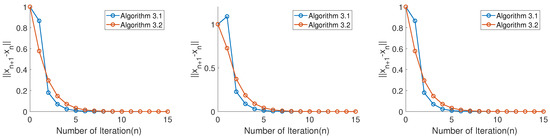
Figure 1. Three initial cases for ${\theta }_n = 0.5 + 1/(n+1)$.

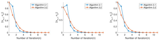
Figure 2. Three initial cases for ${\theta }_n = 1$.

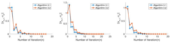
Figure 3. Three initial cases for ${\theta }_n = 0$.

Table 1. Time and iterations of Algorithms 1 and 2 in Ex.1.

	Algorithm	Case I	Case II	Case III
		(sec.)/(n)	(sec.)/(n)	(sec.)/(n)
${\theta }_n = 0$	Algorithm 1	4.26/16	4.75/18	4.78/18
	Algorithm 2	4.80/18	9.35/20	1.67/22
${\theta }_n = 0.5 + \frac{1}{(n+1)}$	Algorithm 1	4.19/12	4.96/12	4.27/12
	Algorithm 2	4.23/16	16.37/18	10.69/18
${\theta }_n = 1$/(n)	Algorithm 1	2.56/10	2.63/10	2.60/10
	Algorithm 2	3.17/12	3.25/12	3.25/12

Example 2.

We consider an examplewhich is from the realm of compressed sensing. More specifically, we try to recover the K-sparse original signal $x_0$ from the observed signal b.

Here, matrix $T\in R^{m\ast n}$, $m<<n$ would be involved and created by standard Gaussian distribution. The observed signal $b = Tx + ϵ$, where $ϵ$ is noise. For more details on signal recovery, one can consult Nguyen and Shin [31].

Conveniently, solving the above sparse signal recovery problem is usually equivalent to solving the following LASSO problem (see Gibali et al. [32] and Moudafi et al. [33]):

$$\begin{array}{cc}& {min}_{x\in R^n}{\parallel Tx-b\parallel }^2\\ & {s.t.\parallel x\parallel }_1\le t,\end{array}$$

where t is a given positive constant. If we define

$$A\left(x\right) =\left\{\begin{array}{cc}\{u:\underset{{\parallel x\parallel }_1\le t}{sup}⟨x-y,u⟩\le 0\},\hfill & \mathrm{if}y\in R^n,\hfill \\ \varnothing ,\hfill & \mathrm{otherwise},\hfill \end{array}\right.B\left(x\right) =\left\{\begin{array}{cc}{R}^m,\hfill & \mathrm{if}x = b,\hfill \\ \varnothing ,\hfill & \mathrm{otherwise},\hfill \end{array}\right.$$

then one can see that the LASSO problem coincides with the problem of finding $x^{\ast }\in R^n$ such that

$$0\in A\left(x^{\ast }\right)\mathrm{and}0\in B\left(T{x}^{\ast }\right).$$

During the operation, $T\in R^{m\ast n}$ is generated randomly with $m = 2^{15}, 2^7$, $n = 2^{16}, 2^8$, $x_0\in R^n$ is K-spikes $(K = 100, 50)$ with amplitude $\pm 1$ distributed throughout the region randomly. In addition, the signal to noise ratio (SNR) is chosen as $SNR = 40$, ${\alpha }_n = 0.5 + 1/(10n+2)$ in two algorithms and ${\gamma }_n = 1/n$ in Algorithm 2. The recovery simulation results are illustrated in Figure 4.

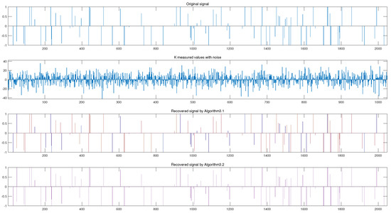
Figure 4. Numerical results for $m = 2^{15}, m = 2^{16}$, and $K = 100$.

Moreover, we also compare our algorithms with the results of Sitthithakerngkiet et al. [21], Kazimi and Riviz. [22], Byrne et al. [5] which have no inertial item and Tang [34] with a general inertial method.

For simplicity, for Algorithm 3.1 in Sitthithakerngkiet et al. [21], the nonexpansive mappings $S_n$ are defined as $S_n = I$, $D = I$, $\xi = 0.5$, and $u = 0.1$, the parameters ${\alpha }_n = \frac{1}{n+1}$ and ${\beta }_n = 0.5 - \frac{1}{10n+2}$. For Algorithm 3.1 in Sitthithakerngkiet et al. [21], Kazimi and Riviz [22], and Algorithm 3.1 in Byrne et al. [5], the step size $\gamma = \frac{1}{L}$, where $L = \parallel T^{\ast }T\parallel$. For Algorithms 3.1 and 3.2 in Tang [34], the step size is self-adaptive, and ${\alpha }_n = 0.5 + 1/(10n+2), {\gamma }_n = 1/n$. The experiment results are illustrated in Figure 5 and Table 2.

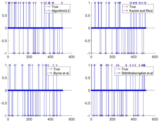
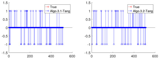
Figure 5. Numerical results for $m = 2^7, m = 2^9$, and $K = 50$.

Table 2. Comparisons of Algorithm 3.1, Algorithm 3.2, and Algorithm 3.1 in Sitthithakerngkiet [21], Algorithm 3.1 in Byrne [5], Algorithm 3.1 in Kazimi and Riviz [22], and Algorithms 3.1 and 3.2 in Tang [34].

DOL	Method	Iter (n)	CPU Time (s)
${10}^{-4}$	Algorithm 1	3	0.019
	Algorithm 2	65	0.19
	Algorithm 3.1-Tang [34]	3	0.14
	Algorithm 3.2-Tang [34]	35	2.26
	Sitthithakerngkiet [21]	78	0.12
	Byrne et al. [5]	2	0.01
	Kazimi and Riviz [22]	48	0.08
${10}^{-5}$	Algorithm 1	3	0.017
	Algorithm 2	102	0.24
	Algorithm 3.1-Tang [34]	8	2.37
	Algorithm 3.2-Tang [34]	76	2.78
	Sitthithakerngkiet [21]	1272	3.03
	Byrne et al. [5]	3	0.013
	Kazimi and Riviz [22]	503	0.74

From Table 2, we can see that our Algorithms 1 and 2 seem to have some competitive advantages.

Compared with the general inertial methods, the main advantage of our Algorithms 1 and 2 in this paper, as mentioned in the previous sections, is that they have no constraint on the norm of the difference between $x_n$ and $x_{n-1}$ in advance, and no assumption on the inertial parameter ${\theta }_n$, so it is extremely natural, attractive, and user friendly.

Moreover, when we test Algorithm 3.1 of Sitthithakerngkiet et al. [21], Algorithm 3.1 of Byrne et al. [5], and Kazimi and Riviz [22], we find that the convergence rate depends strongly on the step size $\gamma$, which depends on the norm of linear operator T, so another advantage of our Algorithms 1 and 2 in this paper is the self-adaptive step size.

5. Conclusions

We proposed two new self-adaptive inertial-like proximal point algorithms (Algorithms 1 and 2) for the split common null point problem (SCNPP). Under more general conditions, the weak and strong convergences to a solution of SCNPP are obtained. The new inertial-like proximal point algorithms listed are novel in the following ways:

(1)

Different from the average inertia technique, the convergence of the proposed algorithms remain even if without the term below:

$$\sum _{n=1}^{\infty }{\theta }_n{\parallel x_n-x_{n-1}\parallel }^2 < \infty .$$

They do not need to calculate the values of $\parallel x_n-x_{n-1}\parallel$ in advance if one chooses the coefficients ${\theta }_n$, which means that the algorithms are easy to use.

(2)

The inertial factors ${\theta }_n$ can be chosen in $[0,1]$, which means that ${\theta }_n$ is a possible equivalent to 1 and opens a wider path for parameter selection.

(3)

The step sizes of our inertial proximal algorithms are self-adaptive and are independent of the cocoercive coefficients, which means that they do not use any prior knowledge of the operator norms.

In addition, two numerical examples involving comparison results have been expressed to show the efficiency and reliability of the listed algorithms.

References

- Censor, Y.; Elfving, T. A multiprojection algorithm using Bregman projections in product space. Numer. Algorithms 1994, 8, 221–239. [Google Scholar] [CrossRef]
- Moudafi, A. Split monotone variational inclusions. J. Optim. Theory Appl. 2011, 150, 275–283. [Google Scholar] [CrossRef]
- Byrne, C. Iterative oblique projection onto convex sets and the split feasibility problem. Inverse Probl. 2002, 18, 441–453. [Google Scholar] [CrossRef]
- Moudafi, A.; Thakur, B.S. Solving proximal split feasibilty problem without prior knowledge of matrix norms. Optim. Lett. 2013, 8. [Google Scholar] [CrossRef] [Green Version]
- Byrne, C.; Censor, Y.; Gibali, A.; Reich, S. Weak and strong convergence of algorithms for the split common null point problem. J. Nonlinear Convex Anal. 2012, 13, 759–775. [Google Scholar]
- Alvarez, F.; Attouch, H. An inertial proximal method for maximal monotone operators via discretization of a nonlinear oscillator with damping. Set-Valued Anal. 2001, 9, 3–11. [Google Scholar] [CrossRef]
- Alvarez, F. Weak convergence of a relaxed and inertial hybrid projection-proximal point algorithm for maximal monotone operators in Hilbert spaces. SIAM J. Optim. 2004, 14, 773–782. [Google Scholar] [CrossRef]
- Attouch, H.; Chbani, Z. Fast inertial dynamics and FISTA algorithms in convex optimization, perturbation aspects. arXiv 2016, arXiv:1507.01367. [Google Scholar]
- Attouch, H.; Chbani, Z.; Peypouquet, J.; Redont, P. Fast convergence of inertial dynamics and algorithms with asymptotic vanishing viscosity. Math. Program. 2018, 168, 123–175. [Google Scholar] [CrossRef]
- Attouch, H.; Peypouquet, J.; Redont, P. A dynamical approach to an inertial forward-backward algorithm for convex minimization. SIAM J. Optim. 2014, 24, 232–256. [Google Scholar] [CrossRef]
- Akgül, A. A novel method for a fractional derivative with non-local and non-singular kernel. Chaos Solitons Fractals 2018, 114, 478–482. [Google Scholar]
- Hasan, P.; Sulaiman, N.A.; Soleymani, F.; Akgül, A. The existence and uniqueness of solution for linear system of mixed Volterra-Fredholm integral equations in Banach space. AIMS Math. 2020, 5, 226–235. [Google Scholar] [CrossRef]
- Khdhr, F.W.; Soleymani, F.; Saeed, R.K.; Akgül, A. An optimized Steffensen-type iterative method with memory associated with annuity calculation. Eur. Phys. J. Plus 2019, 134, 146. [Google Scholar] [CrossRef]
- Ochs, P.; Chen, Y.; Brox, T.; Pock, T. iPiano: Inertial proximal algorithm for non-convex optimization. SIAM J. Imaging Sci. 2014, 7, 1388–1419. [Google Scholar] [CrossRef]
- Ochs, P.; Brox, T.; Pock, T. iPiasco: Inertial proximal algorithm for strongly convex optimization. J. Math. Imaging Vis. 2015, 53, 171–181. [Google Scholar] [CrossRef]
- Dang, Y.; Sun, J.; Xu, H.K. Inertial accelerated algorithms for solving a split feasibility problem. J. Ind. Manag. Optim. 2017, 13, 1383–1394. [Google Scholar] [CrossRef] [Green Version]
- Soleymani, F.; Akgül, A. European option valuation under the Bates PIDE in finance: A numerical implementation of the Gaussian scheme. Discret. Contin. Dyn. Syst.-S 2018, 13, 889–909. [Google Scholar] [CrossRef] [Green Version]
- Suantai, S.; Srisap, K.; Naprang, N.; Mamat, M.; Yundon, V.; Cholamjiak, P. Convergence theorems for finding the split common null point in Banach spaces. Appl. Gen. Topol. 2017, 18, 3345–3360. [Google Scholar] [CrossRef] [Green Version]
- Suantai, S.; Pholasa, N.; Cholamjiak, P. The modified inertial relaxed CQ algorithm for solving the split feasibility problems. J. Ind. Manag. Optim. 2017, 14, 1595. [Google Scholar] [CrossRef] [Green Version]
- Dong, Q.L.; Cho, Y.J.; Zhong, L.L.; Rassias, T.M. Inertial projection and contraction algorithms for variational inequalities. J. Glob. Optim. 2018, 70, 687–704. [Google Scholar] [CrossRef]
- Sitthithakerngkiet, K.; Deepho, J.; Martinez-Moreno, J.; Kumam, P. Convergence analysis of a general iterative algorithm for finding a common solution of split variational inclusion and optimization problems. Numer Algorithms 2018, 79, 801–824. [Google Scholar] [CrossRef]
- Kazmi, K.R.; Rizvi, S.H. An iterative method for split variational inclusion problem and fixed point problem for a nonexpansive mapping. Optim. Lett. 2014, 8, 1113–1124. [Google Scholar] [CrossRef]
- Promluang, K.; Kumam, P. Viscosity approximation method for split common null point problems between Banach spaces and Hilbert spaces. J. Inform. Math. Sci. 2017, 9, 27–44. [Google Scholar]
- Ealamian, M.; Zamani, G.; Raeisi, M. Split common null point and common fixed point problems between Banach spaces and Hilbert spaces. Mediterr. J. Math. 2017, 14, 119. [Google Scholar] [CrossRef]
- Aoyama, K.; Kohsaka, F.; Takahashi, W. Three generalizations of firmly nonexpansive mappings: Their relations and continuity properties. J. Nonlinear Convex Anal. 2009, 10, 131–147. [Google Scholar]
- Xu, H.K. Iterative algorithms for nonliear operators. J. Lond. Math. Soc. 2002, 66, 240–256. [Google Scholar] [CrossRef]
- Maingé, P.E. Approximation methods for common fixed points of nonexpansive mappings in Hilbert spaces. J. Math. Anal. Appl. 2007, 325, 469–479. [Google Scholar] [CrossRef] [Green Version]
- Opial, Z. Weak convergence of the sequence of successive approximations for nonexpansivemappings. Bull. Am. Math. Soc. 1967, 73, 591–597. [Google Scholar] [CrossRef] [Green Version]
- Maingé, P.E. Strong convergence of projected subgradient methods for nonsmooth and nonstrictly convex minimization. Set-Valued Anal. 2008, 16, 899–912. [Google Scholar] [CrossRef]
- Censor, Y.; Gibali, A.; Reich, S. Algorithms for the split variational inequality problem. Numer. Algorithms 2012, 59, 301–323. [Google Scholar] [CrossRef]
- Nguyen, T.L.N.; Shin, Y. Deterministic sensing matrices in compressive sensing: A survey. Sci. World J. 2013, 2013, 192795. [Google Scholar] [CrossRef] [PubMed] [Green Version]
- Gibali, A.; Liu, L.W.; Tang, Y.C. Note on the modified relaxation CQ algorithm for the split feasibility problem. Optim. Lett. 2018, 12, 817–830. [Google Scholar] [CrossRef]
- Moudafi, A.; Gibali, A. l1 − l2 Regularization of split feasibility problems. Numer. Algorithms 2018, 78, 739–757. [Google Scholar] [CrossRef] [Green Version]
- Tang, Y. New inertial algorithm for solving split common null point problem in Banach spaces. J. Inequal. Appl. 2019, 2019, 17. [Google Scholar] [CrossRef] [Green Version]
Publisher’s Note: MDPI stays neutral with regard to jurisdictional claims in published maps and institutional affiliations. |
© 2021 by the authors. Licensee MDPI, Basel, Switzerland. This article is an open access article distributed under the terms and conditions of the Creative Commons Attribution (CC BY) license (https://creativecommons.org/licenses/by/4.0/).