1. Introduction
The construction and study of analytically solvable models for nonlinear wave dynamics of deformable systems is a complicated multi-factorial problem, which has led to the development of non-classical mathematical physics, computational mathematics, and non-destructive testing methods in acoustics. A solvable model is understood as a model that allows the construction of exact analytical solutions. According to [
1], two main methods are available to obtain a solvable model: simplifying hypotheses into complete equations of the three-dimensional elasticity theory with the further asymptotic integration [
2,
3] and the simplification of the available model using a correct asymptotic procedure [
4]. The second approach is used in this work.
Notwithstanding the extensive use of computational simulations, which enable integrally describing the physical process, the possibility of a qualitative analysis is crucial for distinguishing physically significant effects and obtaining the simplest possible mathematical formulation of a problem. It is known that solutions of nonlinear equations are very sensitive to nonlinear terms and to the values of coefficients for them, complicating the verification of numerical methods [
5]. Furthermore, general computational solutions have properties described by particular, exact, and asymptotic solutions [
5,
6]. Finally, exact particular solutions are useful for analyzing the dispersion and dissipation properties of difference schemes, in terms of the differential approximation method [
7].
The constructed model can be considered advantageous, if exact analytical solutions provide clear understanding of a physical phenomenon. It is the very case when computational simulations enable confirming, specifying, or even rejecting original hypotheses [
8]. This article focuses on the discussions of some of the problems that arise when modeling a particular class of problems, regarding the propagation of nonlinear waves in the Timoshenko-type thin elastic cylindrical shells [
9] interacting with a nonlinear elastic Winkler medium [
4,
10,
11]. This article is arranged as follows. In the first section, a solvable model is obtained and the exact solutions thereof cannot be physically realized. In the second section, asymptotics are introduced, which enable constructing models, supposing the existence of exact physically realizable solutions in the form of traveling periodic waves. The third section focuses on the study of the modulation instability of periodic waves. The conclusion is a discussion of the results.
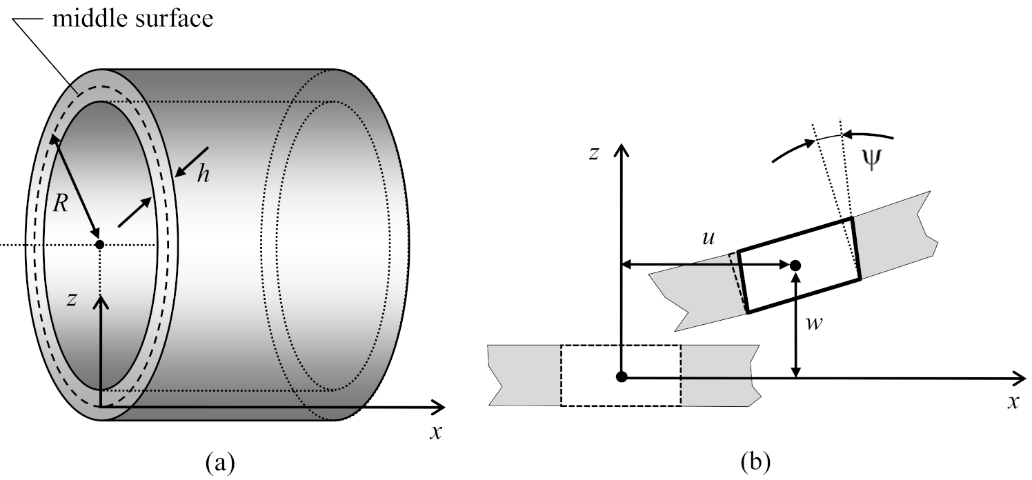
2. Formulation of the Problem
Let us consider the system of equations [
12] for axisymmetric deformations of the Timoshenko-type circular cylindrical shell surrounded by the nonlinear elastic Winkler medium:
The coordinate axes
and
are directed, respectively, along the longitudinal axis of the shell and along its radius towards the cross section center (
Figure 1a). The motions of the shell’s middle surface elements along the axes
and
are designated as
u and
w (
Figure 1b). The other designations shall be as follows:
is the angle of rotation of the normal to the middle surface of the shell;
E,
and
are Young’s modulus, Poisson’s ratio, and the specific gravity of the shell material;
R and
h are the radius of the shell curvature and the shell wall thickness;
g is the gravitational acceleration;
t is time;
is the dimensionless correction factor of the Timoshenko model;
are coefficients characterizing the law of the external environment deformation.
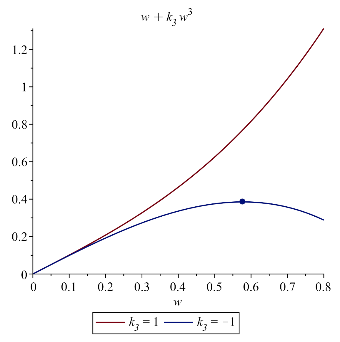
The elastic limit (that is the maximum deformation after the removal thereof no permanent residual deformations emerge) and the proportionality limit (the maximum deformation whereunder Hooke’s law is implemented) practically coincide in conventional structural materials, such as concrete and steel. The propagation of elastic waves in such materials is adequately described by a linear physical model. However, many modern synthetic materials are elastically deformed far beyond the linear zone; thus, nonlinear physical models shall be used for such materials [
13]. One of the basic models of the nonlinear deformation law is based on the polynomial stress–strain (or stress–displacement) relationship. The right hand side of the Equation (
2) sets the cubic deformation law for a nonlinear elastic medium resisting the radial displacement of the shell element [
14]; here, we neglect the resistance of the medium to longitudinal displacement
u, assuming that
can be taken for the propagation of nonlinear elastic waves with their amplitude comparable to the shell thickness.
The linear resistance factor of the medium
is always positive; the coefficient of the nonlinear term
can have any sign. At
, the so-called event of hard nonlinearity is realized, whereat the instantaneous modulus of the medium elasticity increases with enhancing deformations. The “stress–displacement” deformation law
is represented by a monotonic increasing curve over the entire range of displacements. In case of the soft nonlinearity at
, the deformation law has a decreasing segment (
Figure 2). If the displacement modulus
w can exceed the cubic dependence maximum
marked by a dot in
Figure 2, the functional “stress–displacement” relationship loses its mutual uniqueness. Therefore, in case of the soft nonlinearity, the permissible displacement values are limited by the following inequality
The system of nonlinear Equations (
1)–(
3) apparently has no exact solutions. We now try to find its physically admissible approximate solutions using methods of asymptotic integration and multiple scales [
15].
An infinite thin-walled circular cylindrical shell has an obvious small geometric dimensionless parameter equal to the shell thickness-to-radius ratio [
2,
3,
16]:
Let us rewrite the system under consideration in a dimensionless form by scaling the variables with the aid of parameter , so the approximate system of equations arising in principal orders for could be reduced to a single resolving equation. In the course of scaling, we require compliance with the following conditions:
Functions w, and have the same order of smallness;
The inertia of longitudinal displacements and turns are negligible;
The terms containing the correction coefficient of the Timoshenko-type model and the nonlinear coefficient of the external medium resistance shall be included in the resolving equation;
The system of three equations obtained during the transformations should not lose coherence.
The first condition is standard in the theory of flexible thin shells, wherein the rotation angle
associated with transverse displacement is considered far larger than the value of the derivative
related to deformation in the bulk of the shell material and the square of the derivative
is of the same order as
[
12]. The second and third conditions mean that we are interested in transverse nonlinear waves emerging in Timoshenko-type shells. Finally, the fourth condition guarantees that the functional relationship is preserved between the dependent variables
w,
u, and
; all of them can be determined from the solution of the problem.
To satisfy the above conditions, it is required to perform in system (
1)–(
3) a transition to new dimensionless variables
and non-dimensional factors
where
p is an arbitrary constant. New dimensionless dependent variables, their derivatives for
,
, and non-dimensional factors shall be of the order of unity, so as to be able to sort the terms in the system by small parameter
powers.
3. The First Asymptotics
When choosing
in (
6) and (
7), the system of Equations (
1)–(
3) is transformed to the form of
The main part of Equation (
10) contains three terms. Dropping the term
, we integrate (
8) according to
, assuming the integration constant to be zero and express
as follows:
After substituting (
11) into (
9), the last equation is greatly simplified as it just contains a single nonlinear term characterizing the effect of a nonlinear elastic medium:
We express
from (
12) and substitute the result into Equation (
10), having previously differentiated thereof for
. Neglecting the term
, we finally obtain
The nonlinear fourth order equation is a resolving one for the main order of system (
8)–(
10), with respect to the small parameter
. This equation can be called the generalized Boussinesq–Ostrovsky equation, since it contains dispersion terms specific to the usual and “improved” Boussinesq equation [
17], as well as a linear term proportional to W, typical of the Ostrovsky equation [
18,
19,
20,
21].
To find the exact solutions for Equation (
13), we use the traveling wave variable
:
The substitution of
into the leading terms of Equation (
14), containing the highest derivative and the highest nonlinearity, shows that the balance of the leading terms is achieved at
. It means that the solution of Equation (
14) has a simple pole.
To find the exact solutions for non-integrable equations, many effective methods have been developed by now [
22,
23]. According to the popular truncated decomposition method, a solution with the order pole
q shall be sought in the form of a complete polynomial according to some basic functions
with the eigenorder of the pole
:
so that
. Using the Jacobi elliptic function
with simple zeros and poles as a basic function, we will seek a solution to Equation (
14) in the form
where
are arbitrary constants. Substituting (
16) into (
14) and equating coefficients to zero at the same degrees of
, we obtain the following nonlinear system of equations
Using the package of symbolic mathematics, Maple, it was found that:
However, it is required in each of these sets of conditions that the correction factor of the Timoshenko-type model shall be zero or negative, or the nonlinear coefficient of the external medium resistance shall be equal to zero. The said requirements contradict the scaling conditions introduced hereinabove and, therefore, these solutions are not physically realizable.
4. The Second Asymptotics
When choosing
, the principal part of the third equation of system (
1)–(
3) contains, after scaling, only two terms. For example, at
we obtain
Dropping the term
, we integrate (
18) according to
, designating the integration constant as
and express
as follows:
Further, we will consider, separately, two options with zero and nonzero integration constant. Note that, in a similar situation, when considering the first asymptotics, only the zero integration constant was analyzed. Thus, if in the case of the first asymptotics, the integration constant is taken to be nonzero, then we cannot find meaningful particular solutions for the resolving equation.
After substituting (
21) into (
19), the last equation shall become
Having expressed
from (
22) and substituted the result into the principal part of (
20), we obtain the Klein–Gordon nonlinear/non-homogeneous equation
4.1. Variant 1.
In this case, the general solution of (
23) may be written as:
where
and
are two arbitrary functions. Both the amplitude and the second argument of the function
(elliptic modulus), which determines the solution period, shall depend on the function
. It is easy to verify that the expression for the partial derivative
contains the so-called secular term
increasing without limit in module at
. A stationary wave process in the shell is therefore possible only provided that
To obtain the reasonable sorting of the terms of system (
18)–(
20), with the further dropping of the terms containing
, it is necessary, first, that the differentiation, with respect to
or
, would not change the order of smallness for dependent variables
W,
U, and
, and second—that all non-dimensional factors would be of order
.
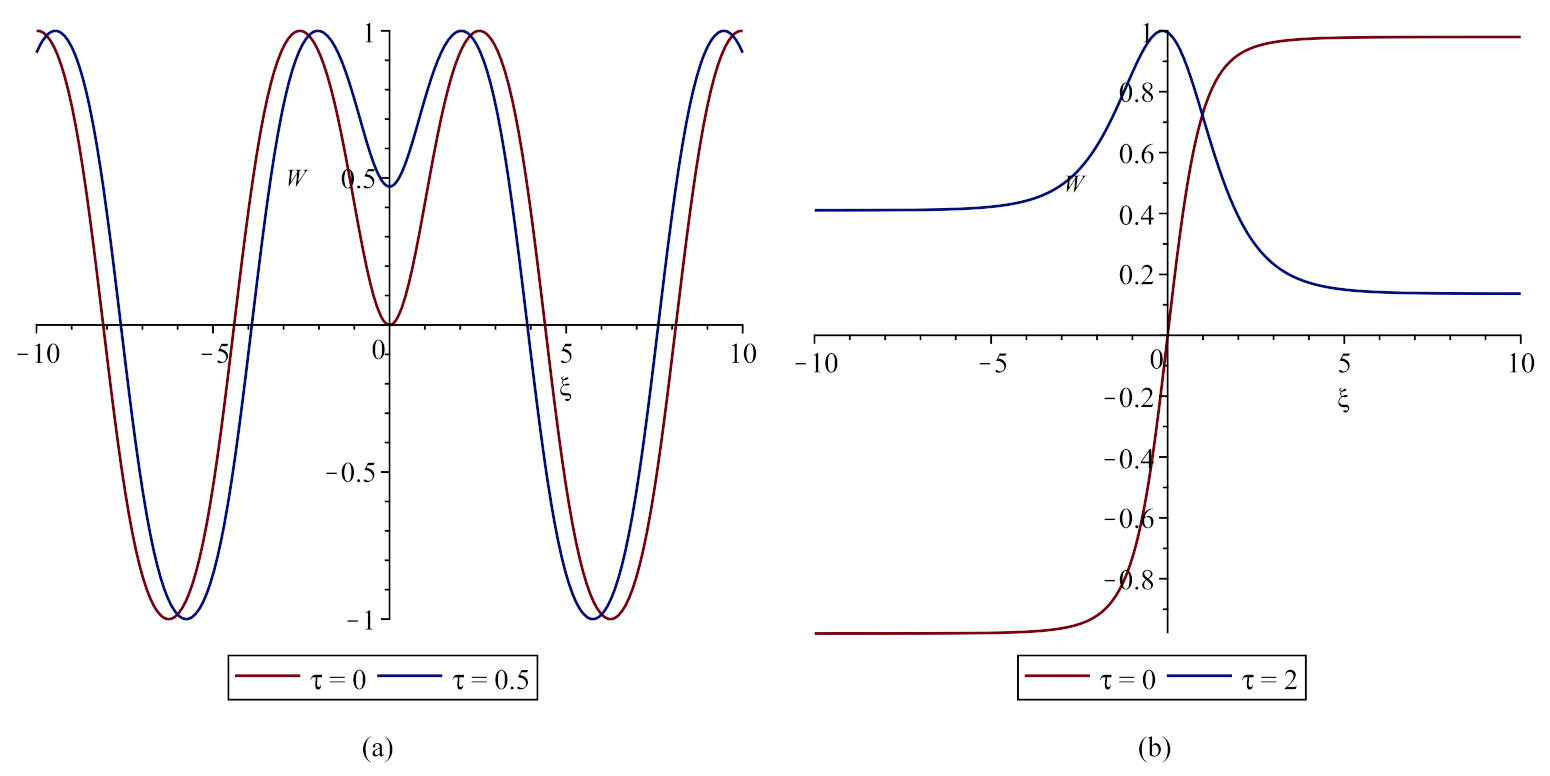
Assuming that
, functions
W and
have the same order, if
Thus, any function is suited as
, if the modulus of its derivative is bounded by a constant of the order of unity. In particular, when choosing
, the solution (
24) determines a stationary traveling wave. When choosing
, we obtain a combination of two traveling waves moving towards each other (
Figure 3a); for the case of
, we have a combination of two “pedestals” vibrating in opposite phases (
Figure 3b).
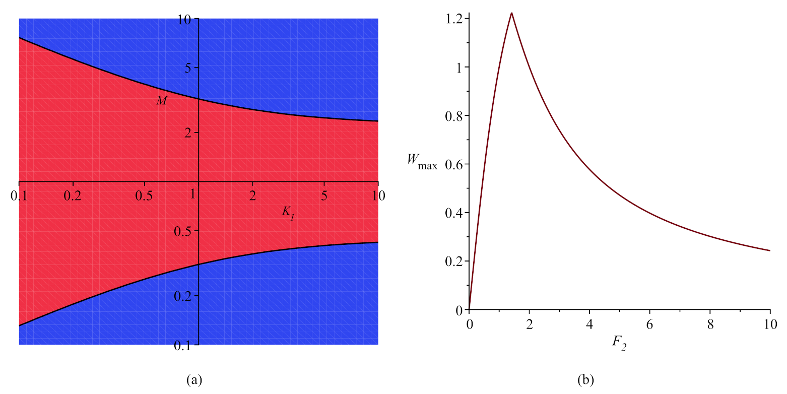
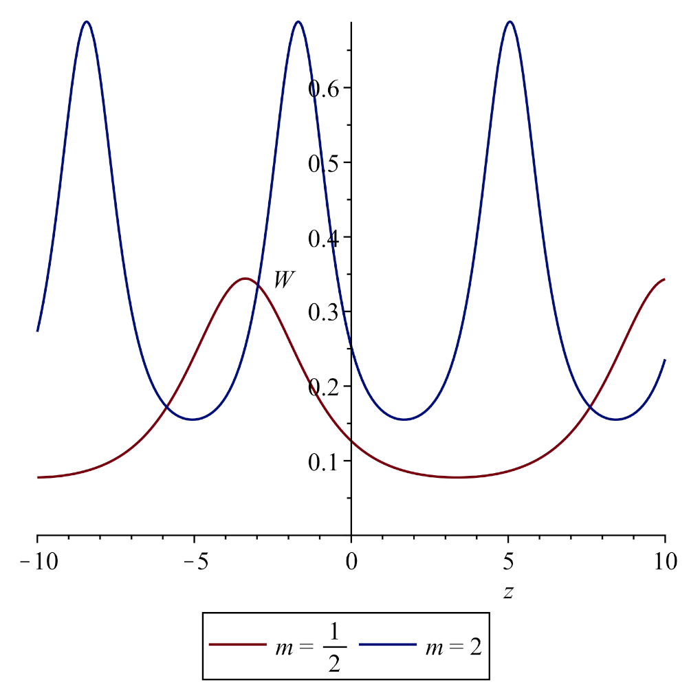
Limiting ourselves to considering the positive values of
,
and the elliptic modulus
of the function
in solution (
24), we ascertain the conditions, whereunder this solution is physically realizable. Obviously, in the case under consideration, the inequality
must be satisfied; it means that the medium has a soft nonlinearity [
11,
24,
25,
26]. The physicality requirement (
4) can be represented as follows
Inequalities (
29) imply the constraints for the elliptic modulus
the areas of the implementation thereof are shown in blue in
Figure 4a.
Thus, the solution does not lack physicality at small or large values of the parameter
M, and solitary waves (
) cannot emerge in the system. The graph in
Figure 4b shows how the amplitude
of the solution depends on the parameter
. Both, in case of
and in case of
, the amplitude
tends to zero, and the graph of the elliptic function
approaches the graph of
.
4.2. Variant 2.
The general solution to (
23) may not be found in this case. After the transition to the traveling wave variable
, Equation (
23) assumes the reduction of order by integration for variable
z:
where
and
is the constant of integration. Equation (
31) generalizes the canonical equation for the function
and its particular solution can be found in the form of
Substituting (
33) into (
31) after grouping in powers of
, we obtain the following system of equations
the exact nontrivial solution thereof with consideration of equalities (
32) takes the form of
Here (and elsewhere), without limiting the generality, we assume that .
We now ascertain under what conditions the solutions of (
33), (
35) are physically realizable. First, it follows from the condition of
that
, meaning that this solution only exists at the soft nonlinearity of the external medium. Second, the wave velocity
V is real at
Third, function (
33) is confined at
; this is tantamount to
, where
It is obvious that
for any
m. Finally, the requirement (
4) reduces to the condition of
where
The function
monotonically increases from 0 to
on the interval
and monotonically decreases from
to 10 on the interval
. The condition (
38) is obviously satisfied for any given
, if the parameter
m is small enough. Furthermore, if the right-hand side of the inequality (
38) is greater than 10, such an inequality is valid for sufficiently large values of
m. For any
, there is a neighborhood of the point
, where it is impossible to satisfy (
38). Thus, the situation looks similar to that described in paragraph 4.1, when the physicality conditions are satisfied in two disjoint domains:
m is much less than 1 in one of them and much more than 1 in the other. Notwithstanding the foregoing, the graphs for the solution in the cases
and
are different.
The graphs for solution
in the case
(
Figure 5) have an asymmetric shape and mean values other than zero. The nonzero mean value of the transverse displacement
is a consequence of the introduction of an integration constant
, which emerges when integrating by
of the principal part of (
18):
The left-hand of Equation (
40) is the normal stress
acting in the cross section of the shell and written in dimensionless form. Thus, the nonzero constant
, which has a positive value in case of the soft nonlinearity (
, see (
35)), enables simulating the wave dynamics of the shell subjected to axial tension.
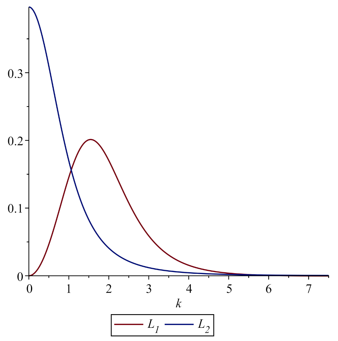
5. The Study of the Modulation Instability
The solitary-wave solutions appear to be physically unrealizable in all of the foregoing asymptotics. However, if it is generally impossible in the first asymptotics to find exact physically realizable solutions, periodic traveling waves are available in the second asymptotics. It seems interesting to consider the stability of the periodic wave propagation. To do this, we use a standard technique—the derivation of the nonlinear Schrödinger equation (NSE) followed by the use of the Lighthill criterion [
27].
The procedure of the NSE derived from the evolutionary equation by the multiscale expansion method is well known [
17]. We will not dwell on its details, but will just present the final result.
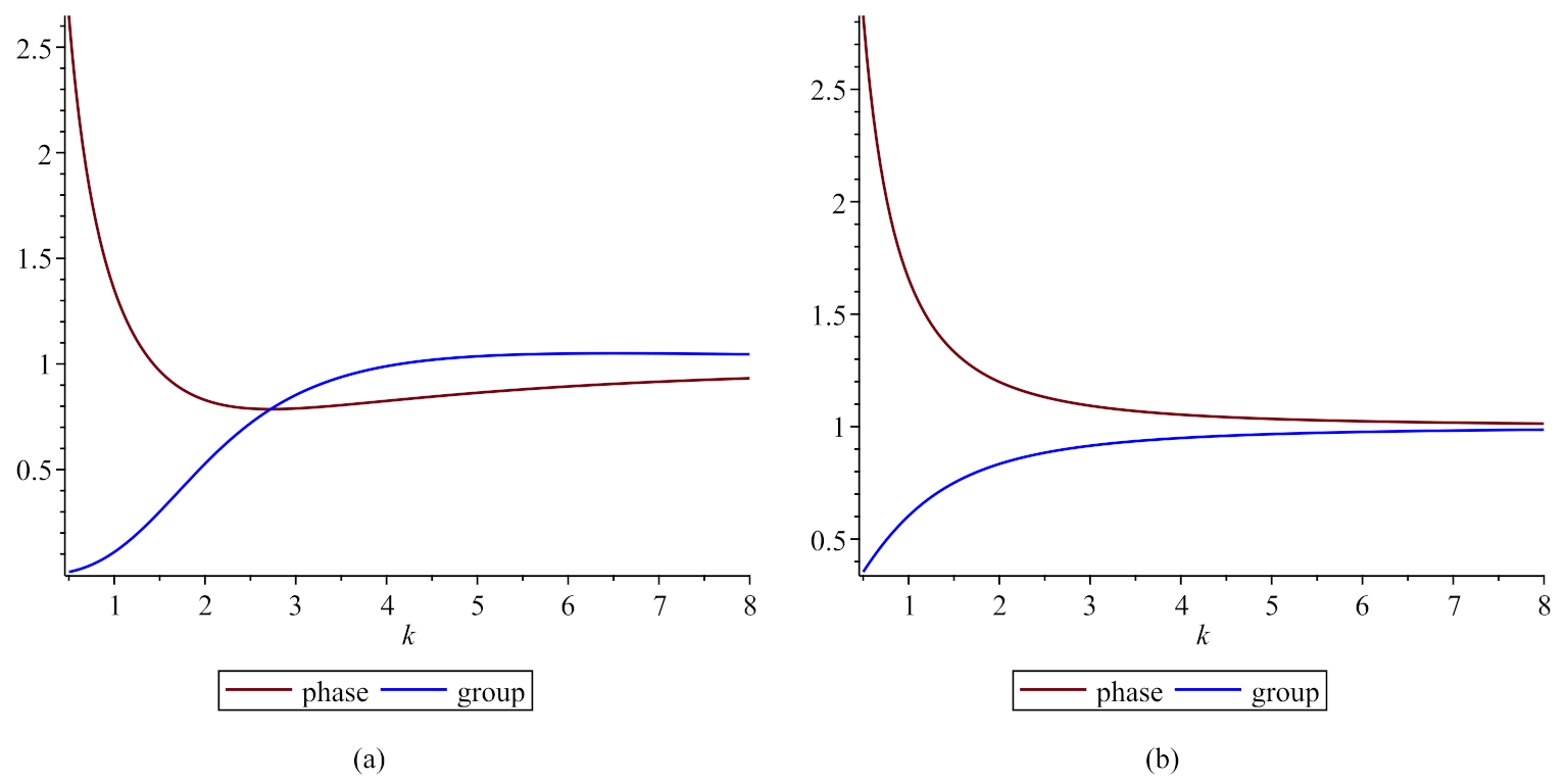
The dispersion relationship between the angular frequency
and the wavenumber
k of linear periodic oscillations for the first asymptotics has the form of
For the second asymptotics it is
The relevant graphs of the phase and group velocities for positive branches of the angular frequency are shown in
Figure 6.
The Lighthill criterion is as follows. If the product
of coefficients of the second derivative and the nonlinear term in the NSE
compiled for the “slow” amplitude
of the linear periodic solution is positive, the modulation instability develops, causing the splitting of a stationary linear wave into a series of “wave packets”. For the first asymptotics, we have
for the second one
Graphs of the relationships
at
and
at
are shown in
Figure 7.
Thus, in case of the first asymptotics, the modulation instability manifests itself at a soft nonlinearity of the environment (). For the second asymptotics, the modulation instability shall be expected in the following two cases: at and (soft nonlinearity, the shell is under axial tension), and at and (hard nonlinearity, the shell is compressed along its axis).
6. Discussion
This article concerns the discussion of the problem of the relationship between the analytical solvability of a mathematical model and the physical realizability of its solutions based on the equations of motion of an element in a Timoshenko-type thin cylindrical shell. The problem is that the formal possibilities for the existence of the exact solutions of the constructed model do not guarantee their physicality, and the impossibility at obtaining exact solutions of a certain class shall not be proof for their physical unrealizability. This "paradox" is explained by the fact that modeling often results in the emergence of non-integrable (in terms of the inverse problem method) equations, the exact particular solutions thereto only exist under special conditions and relations between their coefficients. Such special conditions can contradict the physical meaning of the original problem and forbid the real existence of the obtained solutions. Moreover, the direct numerical simulation can demonstrate the existence of stable solutions with the required properties. However, the conducting of a numerical experiment shall be a separate problem beyond the scope of this article.
The simulation of the axisymmetric propagation of bending waves along the generatrix of the Timoshenko-type elastic cylindrical shell wa carried out using asymptotic integration. Two substantial asymptotics were introduced for consideration, which led to analytically solvable models (in terms of Jacobi elliptic functions). In the first case, the exact solutions were not physical. In the second case, the possibility was ascertained for the real existence of exact solutions in the form of traveling periodic waves of the nonlinear Klein–Gordon equation. This article shows that the obtained solvable models do not have physically realizable solitary-wave solutions. It was determined by the fact that, in the system of a “thin-walled shell–external nonlinear-elastic medium”, dispersion effects greatly surpass nonlinear effects. As a result of the further asymptotic analysis based on the NSE (
43), the possibility of the development of modulation instability was established, leading to the partition of a stationary periodic wave into stable solitary wave packets.


