A Composite Initialization Method for Phase Retrieval

Abstract

Phase retrieval is a classical inverse problem with respect to recovering a signal from a system of phaseless constraints. Many recently proposed methods for phase retrieval such as PhaseMax and gradient-descent algorithms enjoy benign theoretical guarantees on the condition that an elaborate estimate of true solution is provided. Current initialization methods do not perform well when number of measurements are low, which deteriorates the success rate of current phase retrieval methods. We propose a new initialization method that can obtain an estimate of the original signal with uniformly higher accuracy which combines the advantages of the null vector method and maximal correlation method. The constructed spectral matrix for the proposed initialization method has a simple and symmetrical form. A lower error bound is proved theoretically as well as verified numerically.

1. Introduction

Phase retrieval (PR) has many applications in science and engineering, which include X-ray crystallography [1], molecular imaging [2], biological imaging [3], and astronomy [4]. Mathematically, phase retrieval is a problem about finding a signal $\mathit{x}\in {\mathbb{R}}^n$ or ${\mathbb{C}}^n$ satisfying the following phaseless constraints:

$$b_i=\left|⟨a_i,\mathit{x}⟩\right|+{ϵ}_i,i=1,\cdots ,m.$$

(1)

where $b_i\in \mathbb{R}$ is the observed measurement, $a_i\in {\mathbb{R}}^n$ or ${\mathbb{C}}^n$ is the measuring vector, and ${ϵ}_i$ denotes noise. In optics and quantum physics, $a_i$ is related to the Fourier transform or the Fractional Fourier transform [5]. To remove the theoretical barrier, recent works also focus on the generic measurement vectors, namely $a_i\in \mathbb{R}$ independently sampled from $\mathcal{N}(\mathbf{0},{\mathit{I}}_{n\times n})$.

Current methods for solving phase retrieval can be generally divided into two groups: convex and non-convex approaches. Convex methods, e.g., PhaseLift [6] and PhaseCut [7], utilize a semidefinite relaxation to transfer the original problem into a convex one. Nevertheless, the heavy computational cost of these methods hinders its application to practical scenarios. On the other hand, non-convex methods including the Gerchberg–Saxton (GS) [8,9], the (truncated) Wirtinger flow (WF/TWF) [10,11], and the (truncated) amplitude flow (AF/TAF) have a significant advantage in lower computational cost and sampling complexity (i.e., the minimal required $m/n$ to achieve successful recovery) [12]. More recently, two variants of AF using the reweighting [13] and the smoothing technique [14,15] have been proposed to further lower sampling complexity. However, for the mentioned nonconvex methods, the rate of successful reconstruction relies upon elaborate initialization. Moreover, an initialization point nearby the true solution is also a necessity for convergency property in theoretical analysis.

1.1. Prior Art

Current initialization methods for PR problem include spectral method [16], the orthogonality promoting method [12], null vector method [17], and the (weighted) maximal correlation method [13]. These methods first construct a spectral matrix in the form of

$$\mathit{M}=\sum _{i=1}^m{w}_i{a}_i{a}_i^{\mathrm{H}},$$

where the weight $w_i$ is a positive real number. The estimate is then given as the (scaled) eigenvector corresponding to the largest or smallest eigenvalue of $\mathit{M}$. The spectral method and the (weighted) maximal correlation method fall into one category as they seek the leading vector of $\mathit{M}$ as the estimate. We categorize these methods as correlation-focused methods, since their spectral matrices endow more weight to the measuring vectors more correlated to the original signal. Conversely, the null vector and orthogonality promoting method can be regarded as orthogonality-focused methods. For the vector $a_i$ with less correlation to the original signal, the corresponding weight $w_i$ is larger in the spectral matrix.

These two types of initialization methods each have their own merits and demerits. The correlation-focused methods perform better when the oversalting rate $m/n$ is low. While the situation is contrary as $m/n$ is large enough, the orthogonality-focused method provides a more accurate estimate.

1.2. This Work

In this paper, we propose a method combining the advantages of the above two types of initialization methods. Our intuition is to construct a composite spectral matrix, which is a weighted sum of spectral matrices of correlation-focused methods and orthogonality-focused methods. Hence, the new method is termed as the composite initialization method.

1.3. Article Organization and Notations

This paper adopts the following notations. The bold-font lower-case letter denotes a column vector, e.g., $\mathit{b},$$\mathit{z}$. Bold capital letters such as $\mathit{A}$ denote matrices. ${\left(·\right)}^{\mathrm{T}}$ and ${\left(·\right)}^{\mathrm{H}}$ stand for the transpose and the conjugate transpose, respectively. Calligraphic letters such as $\mathcal{I}$ denote a index set, and $\left|\mathcal{I}\right|$ denotes the number of elements of $\mathcal{I}$. ${\left\{a_i\right\}}_{i=1}^m$ is a simple notation of a set of elements in the form of $\left\{a_1,\cdots ,a_m\right\}$. ${∥\mathit{x}∥}_2$ denotes the ${\ell }_2$-norm of $\mathit{x}$. $∥\mathit{x}∥$ means ${∥\mathit{x}∥}_2$ for the sake of simplicity, if not specially specified.

The reminder of this article is organized as follows. The algorithm is given in Section 2. Section 3 provides the theoretical error analysis about the proposed initialization method with some relevant technique error bounds being placed in the Appendix. Section 4 illustrates the numerical performance and makes a comparison of the proposed method with other initialization methods.

2. The Formulation of the Composite Initialization Method

This section provides the formulation of the proposed method. Without loss of generality, we assume that $b_1\le b_2\le \cdots \le b_m.$ Measuring vectors ${\left\{a_i\right\}}_{i=1}^m$ are assumed to be independently sampled centered Gaussian variables with identity covariance for the convenience of theoretical analysis. Let ${\mathit{x}}_0$ be the true solution of (1). For concreteness, we focus on the real-valued Gaussian model. We further assume that $∥{\mathit{x}}_0∥=1$ since this investigation focuses on the estimation of the original signal. In practice, $∥{\mathit{x}}_0∥$ can be estimated by ${∥{\mathit{x}}_0∥}^2\approx \frac{1}{m}{\sum }_1^m{b}_i^2$. To begin with, we describe the null vector and the maximal correlation method which form the basis of our algorithm.

The null vector method first picks out a subset of vectors ${\left\{a_i\right\}}_{i\in {\mathcal{I}}_1}$, where ${\mathcal{I}}_1\subset \left\{1,2,\cdots ,m\right\}$. Then, the null vector method approximates the original signal ${\mathit{x}}_0$ by a vector that is most orthogonal to this subset. Since ${\left\{b_i\right\}}_{i=1}^m$ is in the ascending order, ${\mathcal{I}}_1$ can be directly written as $\left\{1,2,\cdots ,T_1\right\}$, where $T_1$ is the cardinality of ${\mathcal{I}}_1$. The intuition of the null vector method is as simple as follows. Since ${\sum }_{i\in {\mathcal{I}}_1}{\mathit{x}}^{\mathrm{H}}{a}_i{a}_i^{\mathrm{H}}\mathit{x}$ takes a very small value ${\sum }_{i\in {\mathcal{I}}_1}{b}_i^2$ when $\mathit{x}={\mathit{x}}_0$, one can construct the following minimizing problem to estimate ${\mathit{x}}_0$ to coincide this property.

$$\widehat{\mathit{x}}=arg\underset{∥\mathit{z}∥=1}{min}{\mathit{z}}^{\mathrm{H}}\left(\frac{1}{T_1}\sum _{i=1}^{T_1}{a}_i{a}_i^{\mathrm{H}}\right)\mathit{z}.$$

(2)

Solving (2) is equivalent to finding the smallest eigenvalue and the corresponding eigenvector of ${\mathit{M}}_1:=\frac{1}{T}{\sum }_{i=1}^{T_1}{a}_i{a}_i^{\mathrm{H}}$. The so-called orthogonality promoting method proposed by Wang is an approximately equivalent method that transforms the minimization problem (2) into a maximization problem.

The maximal correlation method is based on the opposite intuition, which picks out a subset of vectors ${\left\{a_i\right\}}_{i\in {\mathcal{I}}_2}$ corresponding to the largest $T_2$ elements in ${\left\{b_i\right\}}_{i=1}^m$. As ${\left\{b_i\right\}}_{i=1}^m$ is in the ascending order, ${\mathcal{I}}_2$ can also be written directly as $\left\{m-T_2+1,\cdots ,m\right\}.$ The core idea of maximal correlation method is searching for the vector that is most correlated with ${\left\{a_i\right\}}_{i\in {\mathcal{I}}_2}$. This is achieved by solving the following maximizing problem.

$$\widehat{\mathit{x}}=arg\underset{∥\mathit{z}∥=1}{max}\frac{1}{T_2}\sum _{i=m-T_2+1}^m{\left|⟨a_i,\mathit{z}⟩\right|}^2=arg\underset{∥\mathit{z}∥=1}{max}{\mathit{z}}^{\mathrm{H}}\left(\frac{1}{T_2}\sum _{i=m-T_2+1}^m{a}_i{a}_i^{\mathrm{H}}\right)\mathit{z}.$$

(3)

From (2) and (3), one can observe that these two methods only utilize a subset of vectors that are either most correlated or most orthogonal to the original signal. To make use of as much as possible information, we try to solve a composite problem combining (2) and (3) together.

$$\widehat{\mathit{x}}=arg\underset{∥\mathit{z}∥=1}{min}\left\{{\mathit{z}}^{\mathrm{H}}\left(\frac{1}{T_1}\sum _{i=1}^{T_1}{a}_i{a}_i^{\mathrm{H}}\right)\mathit{z}-\alpha {\mathit{z}}^{\mathrm{H}}\left(\frac{1}{T_2}\sum _{i=m-T_2+1}^m{a}_i{a}_i^{\mathrm{H}}\right)\mathit{z}\right\}.$$

(4)

We can observe that (4) has a symmetrical structure and can be interpreted as a modified version of (2), which adds the objection of (3) as a penalization term. The solution of (4) will be a more accurate estimate than that of (3) since it utilize the information from (2).

Let $H_1={\sum }_{i=1}^{T_1}{b}_i^2/T_1,H_2={\sum }_{i=m-T_2+1}^{T_2}{b}_i^2/T_2$. We set the parameter as $\alpha =H_1/H_2$ in (4). The true signal $\mathit{x}$ is roughly the solution of (2) and (3); thus, it is also the approximated solution of (4). In next section, we will analyze the error of our proposed method.

The algorithm is presented in Algorithm 1. $2\alpha I$ is added to ensure the positivity of $\mathit{M}$. The $x_{k+1}^{\prime }$ in Step 4 is obtained by solving the following system of linear equations:

$$\mathit{M}\mathit{x}={\mathit{x}}_k.$$

(5)

which can be solved by the conjugate descent method since M is a positive and Hermitian by using ${\mathit{x}}_{k-1}$ as initializer.

Since ${\mathit{x}}_0$ and $e^{-i\varphi }{\mathit{x}}_0$ are indistinguishable for the phase retrieval, we evaluate the estimate using the following metric.

$$dist\left(\tilde{\mathit{x}},{\mathit{x}}_0\right)=\underset{\varphi \in [0,2\pi )}{min}\parallel e^{-i\varphi }\tilde{\mathit{x}}-{\mathit{x}}_0\parallel .$$

(6)

The other initialization methods, e.g., the spectral method, the truncated spectral method, and the (weighted) maximal correlation method, are all based on the power iteration. The spectral method is for finding the leading eigenvector of matrix ${\sum }_{i=1}^m{b}_i^2{a}_i{a}_i^T$, which is also realized by the power approach. Chen proposed the truncated spectral method to improve the performance of the spectral method, which constructed another matrix via the threshold parameter $\tau$ [17]. The corresponding matrix for iteration is ${\sum }_{i=1}^m{\mathbf{1}}_{\tau }\left(b_i\right)b_i^2{a}_i{a}_i^{\mathrm{H}}$, where ${\mathbf{1}}_{\tau }$ is defined by the following.    

$${\mathbf{1}}_{\tau }\left(b_i\right)=\left\{\begin{array}{c}1,\mathrm{if}{b}_i\le \tau {∥b∥}_2/\sqrt{m};\hfill \\ 0,\mathrm{else}.\hfill \end{array}\right.$$

(7)

The numerical performance of these initialization methods will be compared later.

Algorithm 1 The composite initialization method.

Input: Increasingly arranged ${\left\{b_i\right\}}_{i=1}^m$ and corresponding ${\left\{a_i\right\}}_{i=1}^m$, truncated value $T_1,T_2$, threshold value $ϵ$, a random initialization ${\mathit{x}}_1$. 1: ${\mathit{M}}_1=\frac{1}{T_1}{\sum }_{i=1}^{T_1}{a}_i{a}_i^{\mathrm{H}}$, ${\mathit{M}}_2=\frac{1}{T_2}{\sum }_{i=T_2+1}^m{a}_i{a}_i^{\mathrm{H}}$, $\alpha =\left(\frac{1}{T_1}{\sum }_{i=1}^{T_1}{b}_i^2\right)/\left(\frac{1}{T_2}{\sum }_{i=m-T_2+1}^m{b}_i^2\right)$ 2: $\mathit{M}={\mathit{M}}_1-\alpha {\mathit{M}}_2+2\alpha \mathit{I}$ 3: for$k=1,2,\cdots$do 4:  $x_{k+1}^{\prime }\leftarrow {\mathit{M}}^{-1}{\mathit{x}}_k$ 5:  ${\mathit{x}}_{k+1}\leftarrow {\mathit{x}}_k^{\prime }/∥{\mathit{x}}_{k+1}^{\prime }∥$ 6:  if $∥{\mathit{x}}_{k+1}-{\mathit{x}}_k∥\le ϵ$, break 7: end for Output:${\mathit{x}}_{\mathrm{OPMP}}={\mathit{x}}_{k+1}/∥{\mathit{x}}_{k+1}∥.$

3. Theoretical Analysis

In this section, we will present the error estimate of the proposed method under Gaussian assumptions in the real case.

Since the measuring vectors are assumed to be i.i.d. Gaussians, we can assume that ${\mathit{x}}_0={\mathit{e}}_1$ without loss of generality, where ${\mathit{e}}_1={[1,0,\cdots ,0]}^{\mathrm{T}}$. Otherwise if ${\mathit{x}}_0\ne {\mathit{e}}_1$, there exists an orthogonal matrix, $\mathit{P}$, satisfying $\mathit{P}{\mathit{x}}_0={\mathit{e}}_1$. Denote $\mathit{A}=\left[a_1,a_2,\cdots ,a_m\right]$, then ${\mathit{A}}^{\mathrm{T}}\mathit{x}={\mathit{A}}^{\mathrm{T}}{\mathit{P}}^T\mathit{P}\mathit{x}$. Let $\mathit{z}=\mathit{Px}$, then the original problem (1) is identical to ${\left(\mathit{PA}\right)}^T\mathit{z}=\mathit{b}$ because $\mathit{PA}$ is composed by Gaussian vectors due to the invariance of Gaussian under the orthogonal transform.

The spectral matrix for orthogonality promoting method is the following.

$${\mathit{M}}_1=\frac{1}{T_1}\sum _{i=1}^{T_1}{a}_i{a}_i^{\mathrm{T}}.$$

(8)

By denoting ${\mathit{d}}_i={\left(a_{i2},a_{i3},\cdots ,a_{in}\right)}^{\mathrm{T}}$, then $\mathit{M}$ can be written as follows:

$${\mathit{M}}_1=\frac{1}{T_1}\sum _{i=1}^{T_1}\left[\begin{array}{cc}{a}_{i1}^2& a_{i1}{\mathit{d}}_i^{\mathrm{T}}\\ a_{i1}{\mathit{d}}_i& {\mathit{d}}_i{\mathit{d}}_i^{\mathrm{T}}\end{array}\right]=\left[\begin{array}{cc}{H}_1& {\mathit{E}}_1^{\mathrm{T}}\\ {\mathit{E}}_1& {\mathit{G}}_1\end{array}\right]$$

(9)

where the following is the case.

$$H_1=\frac{1}{T_1}\sum _{i=1}^{T_1}{a}_{i1}^2,{\mathit{E}}_1=\frac{1}{T_1}\sum _{i=1}^{T_1}{a}_{i1}{\mathit{d}}_i,{\mathit{G}}_1=\frac{1}{T_1}\sum _{i=1}^{T_1}{\mathit{d}}_i{\mathit{d}}_i^{\mathrm{T}}.$$

(10)

The matrix for maximal correlation method is the following:

$${\mathit{M}}_2=\frac{1}{T_2}\sum _{i=m-T_2+1}^m\left[\begin{array}{cc}{a}_{i1}^2& a_{i1}{\mathit{d}}_i^{\mathrm{T}}\\ a_{i1}{\mathit{d}}_i& {\mathit{d}}_i{\mathit{d}}_i^{\mathrm{T}}\end{array}\right]=\left[\begin{array}{cc}{H}_2& {\mathit{E}}_2^{\mathrm{T}}\\ {\mathit{E}}_2& {\mathit{G}}_2\end{array}\right]$$

(11)

where the following is the case.

$$H_2=\frac{1}{T_2}\sum _{i=m-T_2+1}^m{a}_{i1}^2,{\mathit{E}}_2=\frac{1}{T_2}\sum _{i=m-T_2+1}^m{a}_{i1}{\mathit{d}}_i,{\mathit{G}}_2=\frac{1}{T_2}\sum _{i=m-T_2+1}^m{\mathit{d}}_i{\mathit{d}}_i^{\mathrm{T}}.$$

(12)

The constructed matrix for estimation is the following.

$$\mathit{M}={\mathit{M}}_1-\alpha {\mathit{M}}_2,\alpha =H_1/H_2.$$

(13)

To proceed, we notice the following basic facts:

1.

The orthogonality promoting method is for finding the eigenvector of minimum eigenvalue of $\mathit{M}$.

$$\mathit{M}=\left[\begin{array}{cc}0& {\mathit{E}}_1^{\mathrm{T}}-\alpha {\mathit{E}}_2^{\mathrm{T}}\\ {\mathit{E}}_1-\alpha {\mathit{E}}_2& {\mathit{G}}_1-\alpha {\mathit{G}}_2\end{array}\right]:=\left[\begin{array}{cc}0& {\mathit{E}}^{\mathrm{T}}\\ \mathit{E}& \mathit{G}\end{array}\right].$$

(14)

2.

In the ideal case that $\mathit{E}$ is a zero matrix, $\mathit{M}$ degenerates to the following.

$$\tilde{\mathit{M}}=\left[\begin{array}{cc}0& \mathbf{0}\\ \mathbf{0}& \mathit{G}\end{array}\right].$$

If we can also ensure that $\mathit{G}={\mathit{G}}_1-\alpha {\mathit{G}}_2$ is positively definite, the eigenvector corresponding to the smallest eigenvalue is exactly the true signal.

These two facts inspire us to estimate the error by computing the eigenvector of matrix $\tilde{\mathit{M}}$ after adding perturbation $\mathit{E}={\mathit{E}}_1-\alpha {\mathit{E}}_2$. Thus, the outline of theoretical analysis is concluded as follows:

1.

Estimate $\Delta \lambda =\lambda -\tilde{\lambda }$, where $\lambda$ and $\tilde{\lambda }$ are the minimum eigenvalue of $\mathit{M}$ and $\tilde{\mathit{M}}$, respectively;

2.

With $\Delta \lambda$, we can then compute the perturbation of corresponding eigenvector, $\parallel \mathit{v}-\tilde{\mathit{v}}\parallel$, which is the exact error of our algorithm.

Specifically, we have the following roadmap of theoretical analysis. Section 3.1 presents bound results for each component of the spectral matrix $\mathit{M}$. Using the results in Section 3.1, the bounds of $\Delta \lambda$ can then be easily obtained in Section 3.2. The relationship between perturbation of eigenvalues and eigenvectors is presented in Section 3.3, which finally induces the error estimation of our algorithm formally in Section 3.4.

3.1. Analysis of Each Component of the Spectral Matrix

In this part, we will provide the bounds for the variables involved of matrix $\mathit{M}$, which are basic ingredients for estimating perturbation of eigenvalue and eigenvector, namely $\Delta \lambda$ and $\parallel \mathit{v}-\tilde{\mathit{v}}\parallel$. In particular, the upper bound for $H_1$, lower bound for $H_2,$ and the norm of $\mathit{E}$ will be analysed.

3.1.1. Upper Bound of $\alpha =H_1/H_2$

Finding the upper bound of $\alpha$ actually consists in finding the upper bound of $H_1$ and the lower bound of $H_2$. First, we have the upper bound of $H_1$ under statistical meaning in the follow lemma.

Lemma 1.

We have the following:

$$Pr(H_1\le \frac{p_1^2}{4{\rho }_0^2})\ge 1-exp\left(-\frac{m{p}_1^2}{50}\right)$$

(15)

where $p_1=T_1/m$.

The proof of Lemma 1 is placed in the Appendix A and Appendix B. As for the lower bound of $H_2$, we borrow a result from Wang [13], Lemma 3.

Lemma 2.

The following holds with probability exceeding $1-{\mathrm{e}}^{-c_{0}m}$:

$$H_2\ge 0.99(1+log(m/T_2)),$$

(16)

provided that $T_2\ge c_{1}n,m\ge c_2{T}_2$ for some absolute constants $c_0,c_1$, and $c_2$.

Then, we obtained the required upper bound of $H_1/H_2.$

Lemma 3.

Under the set-up of Lemmas 1 and 2, we have the following:

$$\alpha =H_1/H_2\le \frac{p_1^2}{3.96{\rho }_0^2(1-log{p}_2)}$$

(17)

with probability of at least

$$1-exp\left(-\frac{m{p}_1^2}{50}\right)-exp(-c_{0}m),$$

(18)

where ${\rho }_0=1/\sqrt{2\pi }$, $p_1$, and $p_2$ denote $T_1/m$ and $T_2/m$, respectively.

3.1.2. Lower Bound of the Smallest Eigenvalue of $\mathit{G}$

Since $\mathit{G}$ is a linear combination of ${\mathit{G}}_1$ and ${\mathit{G}}_2$, the lower bound of the smallest eigenvalue of $\mathit{G}$ can be estimated from the bounds of eigenvalues of ${\mathit{G}}_1$ and ${\mathit{G}}_2$.

According to (10) and (12), we rewrite ${\mathit{G}}_1$ and ${\mathit{G}}_2$ as the following:

$$\begin{array}{cc}\hfill {\mathit{G}}_1& =\frac{1}{T_1}{\mathit{D}}_1^{\mathrm{T}}{\mathit{D}}_1,{\mathit{G}}_2=\frac{1}{T_2}{\mathit{D}}_2^{\mathrm{T}}{\mathit{D}}_2,\hfill \end{array}$$

(19)

where ${\mathit{D}}_1={[{\mathit{d}}_1,\cdots ,{\mathit{d}}_{T_1}]}^{\mathrm{T}}$ and ${\mathit{D}}_2={[{\mathit{d}}_{m-T_2+1},\cdots ,{\mathit{d}}_m]}^{\mathrm{T}}.$ ${\mathit{D}}_1$ and ${\mathit{D}}_2$ are termed Gaussian matrices here since their entries are all sampled from the Gaussian distribution. We notice that ${\mathit{D}}_1^{\mathrm{T}}{\mathit{D}}_1$ and ${\mathit{D}}_2^{\mathrm{T}}{\mathit{D}}_2$ are Wishart matrices, which can be written as the product of a Gaussian matrix and its adjoint [18]. Moreover, the eigenvalue perturbation of Wishart matrix obeys the following classical result.

Theorem 1

([19], Corollary 5.35). Let $\mathit{A}$ be an $N_1\times N_2$ matrix for which its entries are independent standard normal random variables. Then, for every $t\ge 0$, with a probability of at least $1-2exp\left(-t^2/2\right)$, the following events hold simultaneously:

$$\begin{array}{cc}\hfill & \sqrt{N_1}-\sqrt{N_2}-t\le s_{min}\left(\mathit{A}\right),\hfill \end{array}$$

(20)

$$\begin{array}{cc}\hfill & s_{max}\left(\mathit{A}\right)\le \sqrt{N_1}+\sqrt{N_2}+t,\hfill \end{array}$$

(21)

where $s_{min}\left(\mathit{A}\right)$ and $s_{max}\left(\mathit{A}\right)$ stand for the smallest and the largest singular value of $\mathit{A}$, respectively.

By pplying Theorem 1 to ${\mathit{D}}_1\in {\mathbb{R}}^{T_1\times (n-1)}$ with the following replacements:

(1)

${\mathit{D}}_1\to \mathit{A}$,

(2)

$T_1\to N_1$, $n-1\to N_2$,

(3)

$\sqrt{n-1}/10\to t$,

one can see that the following is the case.

$$\begin{array}{c}\hfill Pr\left(s_{min}\left({\mathit{D}}_1\right)\ge \sqrt{T_1}-1.1\sqrt{n-1}\right)\ge 1-2exp\left(-\frac{n-1}{200}\right).\end{array}$$

(22)

In theoretical analysis, we assume that $T_1$ is large enough such that $\sqrt{T_1}-1.1\sqrt{n-1}\ge 0$. However, it should be observed that setting $T_1\ge n$ suffices to output reasonable estimates as shown in the numerical test. Based on this assumption, one then has the following.

$$\begin{array}{cc}\hfill s_{min}\left({\mathit{G}}_1\right)& =s_{min}\left(\frac{1}{T_1}{\mathit{D}}_1^{\mathrm{T}}{\mathit{D}}_1\right)=\frac{1}{T_1}{s}_{min}^2\left({\mathit{D}}_1\right)\hfill \\ \hfill & \ge \frac{1}{T_1}{(\sqrt{T_1}-1.1\sqrt{n-1})}^2={(1-1.1\sqrt{s_1})}^2\hfill \end{array}$$

(23)

The above holds with probability exceeding $1-2exp(-\frac{n-1}{200})$, where $s_1=(n-1)/T_1$. Similarly, we have the following:

$$\begin{array}{c}\hfill Pr\left(s_{max}\left({\mathit{G}}_2\right)\le {\left(1+1.1\sqrt{s_2}\right)}^2\right)\ge 1-2exp\left(-\frac{n-1}{200}\right)\end{array}$$

(24)

where $s_2=(n-1)/T_2$.

Hence, we obtain the lower bound for the smallest eigenvalue of G.

$$\begin{array}{cc}\hfill s_{min}\left(\mathit{G}\right)& =s_{min}({\mathit{G}}_1-\alpha {\mathit{G}}_2)\ge s_{min}\left({\mathit{G}}_1\right)-\alpha s_{max}\left({\mathit{G}}_2\right)\hfill \\ \hfill & \ge {\left(1-1.1\sqrt{s_1}\right)}^2-\alpha {\left(1+1.1\sqrt{s_2}\right)}^2.\hfill \end{array}$$

(25)

A necessary condition for the validness of our method is $s_{min}\left(\mathit{G}\right)\ge 0,$ which can be satisfied by choosing proper $s_1$ and $s_2.$

3.1.3. The Upper Bound of ${\parallel \mathit{E}\parallel }^2$

Now, let us turn to the estimation of the norm of $\mathit{E}$. We denote each item of $\mathit{E}$ as ${\xi }_k$.

$${\xi }_k=\frac{1}{T_1}\sum _{i=1}^{T_1}{a}_{i1}{a}_{ik}-\frac{\alpha }{T_2}\sum _{i=m-T_2+1}^m{a}_{i1}{a}_{ik}.$$

(26)

Since $a_{ik}$ obeys normal distribution, $H_1=\frac{1}{T_1}{\sum }_{i=1}^{T_1}{a}_{i1}^2$ and $H_2=\frac{1}{T_2}{\sum }_{i=m-T_2+1}^m{a}_{i1}^2$, we can derive the following.

$${\xi }_k\sim \mathcal{N}(0,\frac{H_1}{T_1}+\frac{{\alpha }^2{H}_2}{T_2}).$$

Let ${\psi }_k={\xi }_k/\sqrt{\frac{H_1}{T_1}+\frac{{\alpha }^2{H}_2}{T_2}}$, then ${\psi }_k^2$ obeys chi-squared distribution, which is a sub-exponential distribution. With ${\psi }_k$, we can reform ${∥\mathit{E}∥}_2^2$ as the following.

$${\parallel \mathit{E}\parallel }^2=\left(\frac{H_1(n-1)}{T_1}+\frac{{\alpha }^2{H}_2(n-1)}{T_2}\right)\frac{1}{n-1}\sum _{k=2}^n{\xi }_k^2=\left(H_1{s}_1+H_1\alpha s_2\right)\sum _{k=2}^n\frac{{\xi }_k^2}{n-1}.$$

(27)

The expectation of ${∥E∥}_2^2$ is obviously $H_1(s_1+s_2\alpha )$.

The variance of ${∥E∥}_2^2$ is also needed in order obtain the upper bound of ${∥E∥}_2^2$. To this end, we need to recall the Bernstein-type inequality for sub-exponential random variable.

Theorem 2.

Let $X_1,\cdots ,X_N$ be i.i.d. centered sub-exponential random variables with sub-exponential norm denoted as K. Then, for every $t\ge 0$, we have the following:

$$Pr\left(\frac{1}{N}\left|\sum _{i=1}^N{X}_i\right|\ge t\right)\le 2exp\left[-cNmin\left(\frac{t^2}{K^2},\frac{t}{K}\right)\right]$$

(28)

where $c>0$ is an absolute constant. K is the so-called sub-exponential norm defined as the following.

$$K=\underset{p\ge 1}{sup}\frac{1}{p}\left(\mathbb{E}\right|X_1{{|}^p)}^{1/p},$$

(29)

Define a centered sub-exponential random variable $Z_i={\xi }_i-1$. The sub-exponential norm of $Z_i$ is computed in Appendix C. Appendix C tells that the sub-exponential norm $K=1$ in our case. By replacing $n-1\to N,0.1\to t$ and $K\to 1$ in Theorem 2, one can then conclude the following result.

Theorem 3.

Since $K\le 2$, let $t=0.1$, then we have the following:

$$Pr\left(\frac{1}{n-1}\sum _{i=2}^n{\xi }_i^2-1\ge 0.1\right)\le exp\left(-c\frac{n-1}{100}\right)$$

(30)

where $c>0$ is an absolute constant.

Gathering these results, we have the following theorem.

Theorem 4.

$${∥\mathit{E}∥}^2\le 1.1H_1(s_1+s_2\alpha )$$

(31)

The above holds with the probability stated below:

$$1-exp\left(-c\frac{n-1}{100}\right),$$

(32)

with some absolute constant $c>0$.

3.2. Estimate of $\Delta \lambda$

To make an estimate for $\Delta \lambda$, we first recall a classical result from matrix perturbation theory in [20].

Theorem 5.

Let the following be the case:

$$\mathit{M}=\left[\begin{array}{cc}\mathit{H}& {\mathit{E}}^{\mathrm{T}}\\ \mathit{E}& \mathit{G}\end{array}\right],\tilde{\mathit{M}}=\left[\begin{array}{cc}\mathit{H}& \mathbf{0}\\ \mathbf{0}& \mathit{G}\end{array}\right]$$

(33)

Let the above be Hermitian and set $\eta =min\left|\mu -\nu \right|$ over all $\mu \in \sigma \left(\mathit{H}\right)$ and $\nu \in \sigma \left(\mathit{G}\right)$, where $\sigma \left(\mathit{H}\right)$ stands for the set of eigenvalue of $\mathit{H}$. Then, the following is the case:

$$\underset{1\le j\le n}{max}\left|{\lambda }_j^{\uparrow }-{\tilde{\lambda }}_j^{\uparrow }\right|\le \frac{2{∥\mathit{E}∥}_2^2}{\eta +\sqrt{{\eta }^2+4{∥\mathit{E}∥}_2^2}}.$$

(34)

where ${\lambda }_j^{\uparrow }$ and ${\tilde{\lambda }}_j^{\uparrow }$ are the j-th smallest one among the eigenvalues of $\mathit{M}$ and $\tilde{\mathit{M}}$, respectively.

To ensure the effectiveness of our algorithm, $H_1$ should still be the minimum eigenvalue after adding perturbation in our case. Then, $\eta$ is simply $s_{min}\left(\mathit{G}\right)$ that is bounded by (25). Hence, $\Delta \lambda$ can be estimated by the following.

$$\begin{array}{cc}\hfill \left|\Delta \lambda \right|& \le \underset{1\le j\le n}{max}\left|{\lambda }_j^{\uparrow }-{\tilde{\lambda }}_j^{\uparrow }\right|\le \frac{2{∥\mathit{E}∥}_2^2}{\eta +\sqrt{{\eta }^2+4{∥\mathit{E}∥}_2^2}}\le \frac{2{∥\mathit{E}∥}_2^2}{2\eta }\hfill \\ \hfill & \le \frac{1.1H_1(s_1+\alpha s_2)}{{(1-1.1\sqrt{s_1})}^2-\alpha {(1-1.1\sqrt{s_2})}^2}.\hfill \end{array}$$

(35)

3.3. Computing $\parallel \mathit{v}-\tilde{\mathit{v}}\parallel$

With the upper bound of $\Delta \lambda$, we can now estimate the perturbation of the eigenvector. The minimum eigenvector of $\mathit{M}$ is computed by solving $\left(\mathit{M}-(\lambda +\Delta \lambda ){\mathit{I}}_n\right)\mathit{v}=0$:

$$\left(\mathit{M}-(\lambda +\Delta \lambda ){\mathit{I}}_m\right)\mathit{v}=\left[\begin{array}{cc}-\Delta \lambda & {\mathit{E}}^{\mathrm{T}}\\ \mathit{E}& \mathit{G}-(\lambda +\Delta \lambda ){\mathit{I}}_{n-1}\end{array}\right]\mathit{v}=0,$$

(36)

where ${\mathit{I}}_n$ denotes the $n\times n$ identity matrix here. Without loss of generality, the solution of (36) can be written in the form of $\mathit{v}={\left(1,\delta \mathit{v}\right)}^{\mathrm{T}}$. Then, we have the following.

$$\delta \mathit{v}=-{\left(\mathit{G}-(\lambda +\Delta \lambda ){\mathit{I}}_{n-1}\right)}^{-1}\mathit{E}.$$

(37)

Therefore, $\parallel \mathit{v}-\tilde{\mathit{v}}\parallel$ can be bounded by the following:

$$\begin{array}{cc}\hfill & \parallel \mathit{v}-\tilde{\mathit{v}}{\parallel }^2\le {∥\delta \mathit{v}∥}^2\hfill \\ \hfill \mathrm{(38)}& \hfill \le & {∥{\left(\mathit{G}-(\lambda +\Delta \lambda ){\mathit{I}}_{n-1}\right)}^{-1}∥}^2{\parallel \mathit{E}\parallel }^2\hfill \hfill \mathrm{(39)}& \hfill \le & {∥\mathit{E}∥}^2/\left(\eta -{∥\mathit{E}∥}^2/\eta \right),\hfill \end{array}$$

where (38) is derived based on (37). The form of (39) would be a bit complicated, as stated as follows.

$$\frac{{∥\mathit{E}∥}^2}{\eta -{∥\mathit{E}∥}^2/\eta }\le \frac{1.1H_1(s_1+s_2\alpha )\left({\left(1-1.1\sqrt{s_1}\right)}^2-\alpha {\left(1+1.1\sqrt{s_2}\right)}^2\right)}{{\left({\left(1-1.1\sqrt{s_1}\right)}^2-\alpha {\left(1+1.1\sqrt{s_2}\right)}^2\right)}^2-1.1H_1(s_1+s_2\alpha )}.$$

(40)

3.4. Main Result

Notice that $∥\mathit{v}-\tilde{\mathit{v}}∥$ is exactly $∥{\mathit{x}}_0-\tilde{\mathit{x}}∥$. Then, it is straightforward to induce our main theorem by combining the above results.

Theorem 6 (Main result).

Consider the problem of estimating arbitrary $\mathit{x}\in {\mathbb{R}}^n$ from m phaseless measurements (1) under the Gaussian assumption. Suppose the output of Algorithm 1 is ${\tilde{\mathit{x}}}_0$. If $m\ge c_1{T}_1$, $m\ge c_2{T}_2$, $T_1>n$, and $m\ge T_1+T_2$, then we have the following error estimate for the composite initialization method:

$$\parallel {\mathit{x}}_0-\tilde{\mathit{x}}{\parallel }^2\le \frac{RQ}{R-Q},$$

(41)

with a probability of at least the following:

$$P=1-exp\left(-\frac{m{p}_1^2}{144}{\mathrm{e}}^{\frac{-p_1^2}{2{\rho }_0^2}}\right)-{\mathrm{e}}^{-\frac{m{p}_1^2}{50}}-2{\mathrm{e}}^{-\frac{n-1}{200}}-{\mathrm{e}}^{-c\frac{n-1}{100}}-{\mathrm{e}}^{-c_{0}m},$$

(42)

where the following is the case,

$$\begin{array}{cc}\hfill Q& =1.1p_1^2\left(4{\rho }_0^2(1-log{p}_2)s_1+0.99p_1^2{s}_2\right)(1-log{p}_2),\hfill \end{array}$$

(43)

$$\begin{array}{cc}\hfill R& ={\left[4{\rho }_0^2(1-log{p}_2){(1-1.1\sqrt{s_1})}^2-0.99p_1^2{(1+1.1\sqrt{s_2})}^2\right]}^2,\hfill \end{array}$$

(44)

$p_i=T_i/m,s_i=(n-1)/T_i$ for $i=1,2,$ and some absolute constants $c_0,c_1,c_2,{\rho }_0\ge 0$.

Probability P in (42) can be negative when m and n are too small, which shows the limitation of our analysis since m and n need to be large enough so as to render the probability reasonable. In the extreme case that $p_1,p_2,s_1$ and $s_2$ are close to 0, our error estimation expression (41) can be approximated by a simpler form:

$$\parallel {\mathit{x}}_0-\tilde{\mathit{x}}{\parallel }^2⪅\frac{1.1p_1^2{s}_1}{10{\rho }_0^2}$$

(45)

which is verified by numerical experiments later.

4. Numerical Results

In this section, we test the accuracy of the proposed method and compare it with other methods, including the spectral method, the truncated spectral method, the reweighted maximal correlation method, the null vector method, and the orthogonality method. The sampling vectors $a_i$ and the original signal ${\mathit{x}}_0\in {\mathbb{R}}^{100}$ are independently randomly generated. To eliminate the influence of error brought by estimation of $∥{\mathit{x}}_0∥$, the original signal ${\mathit{x}}_0$ is normalized. We chose $T_1=n,T_2=0.3n$ for numerical experiments for the proposed method. All the following simulation results are averaged over 80 independent Monte Carlo realizations.

Figure 1 provides the RMSE calculated by (6) versus the oversampling rate $m/n$ of the mentioned initialization methods. Obviously, all methods exhibit better performance as $m/n$ increases. In particular, the proposed initialization method outweighs the other methods. When $m/n\ge 10$ roughly, the composite initialization method performs closely as the null vector does, and the convergency behavior coincides with (45). When $m/n\le 10$, the proposed method does not lose its accuracy as dramatically as the null vector method does. The proposed algorithm provides the most accurate estimate when oversampling rate is below the information limit, i.e., $m/n\approx 2$.

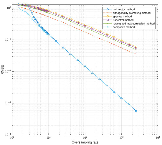
Figure 1. RMSE vs. oversampling rate of several initialization method. $n=100$, $T_1=n,T_2=0.3n$ for the composite initialization method, while for the other algorithms, the involved parameters are selected according to related articles.

Figure 2 illustrates the importance of initialization method on refining the success rate of TAF algorithm [12]. In each simulation, each initialization generates an estimate as the initializer for the TAF algorithm. A trial is considered to be successful if TAF algorithm can return a result with RMSE less than ${10}^{-5}$. When $m/n$ is large, all the presented initialization methods ensure almost 100% success rate. However, when $m/n$ approaches 0, the differences in success rates of various methods appear gradually. Therefore, the composite initialization method can help TAF to achieve better success rate compared with the other two methods.

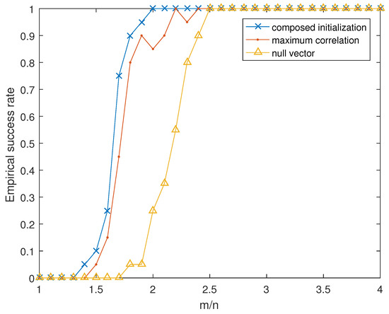
Figure 2. Empirical success rate of different initialization methods versus number of measurements with $n=100$, with $m/n$ varying form 1 to 4 for TAF.

Table 1 illustrates the CPU time needed for the TAF using our method as an initializer compared with other two typical initialization methods. To distinguish the performance more clearly, the length of signal is set as a large number $n=1000$. The proposed method and null vector method need to solve a linear system of equations at each inverse power computation, which makes it more time-consuming than the power computation of the maximal correlation method. However, the proposed method provides a more accurate initializer, which can help TAF converges faster. Hence, the overall efficiency of our algorithm is not far behind power-type methods as shown in Table 1.

Table 1. CPU time (s) for TAF using the proposed initialization method compared with other two typical initializer.

	Method	Initialization Stage	TAF Stage	Overall
	Null vector	1.24	1.34	2.58
$m/n=2$	Maximal correlation	0.47	0.76	1.23
	Proposed	0.72	0.70	1.42
	Null vector	1.12	1.02	2.14
$m/n=3$	Maximal correlation	0.42	0.49	0.91
	Proposed	0.73	0.47	1.2
	Null vector	0.95	1.02	1.97
$m/n=5$	Maximal correlation	0.44	0.45	0.89
	Proposed	0.67	0.46	1.13

5. Conclusions

This paper proposes a new initialization method that combines the advantages of two methods constructed from two totally contrary intuitions. Both theoretical analysis and numerical experiments indicate the validness of our method and higher accuracy compared with other methods. Future work will focus on extending our initialization algorithms to the more generalized problem of PR, e.g., the quadratic sensing and the matrix reconstruction problems [21].

Appendix B.1. The Upper Bound for τ *

Construct the following function.

$$\widehat{\rho }\left(x\right)={\rho }_0\frac{1-\sqrt{x}/2}{\sqrt{x}},$$

(A21)

Then, it can be proved that the following is the case.

$$e^{-x^2/2}>1-x/2,\forall x\in (0,2].$$

(A22)

Therefore, we have the following.

$$\rho \left(x\right)>\widehat{\rho }\left(x\right),\forall x\in (0,4].$$

(A23)

Define $\widehat{F}\left(\tau \right)={\int }_0^{\tau }\widehat{\rho }\left(x\right)dx$. Then, it is obvious that the following is the case.

$$F\left(x\right)>\widehat{F}\left(x\right),\forall x\in (0,4].$$

(A24)

Since $F\left(\tau \right)$ and $\widehat{F}\left(\tau \right)$ are both strictly monotone decreasing over $(0,4]$, their inverse functions satisfy the following:

$${\tau }_{*}=F^{-1}\left(p\right)<{\widehat{F}}^{-1}\left(p\right):=\widehat{\tau },\forall p\in (0,\widehat{F}\left(4\right)].$$

(A25)

where $\widehat{F}\left(4\right)$ is about $0.79$.

In the orthogonality promoting apporach using inverse power, $\left|\mathcal{I}\right|/m$ is always less than 1/2 to achieve a tolerant performance. Therefore, in our concerned range ($0<p<1/2$), it is accessible to estimate ${\tau }_{*}$ by function ${\widehat{F}}^{-1}$.

Now, we compute $\widehat{F}$.

$$\widehat{F}\left(\tau \right)={\int }_0^{\tau }{\rho }_0\frac{1-\sqrt{x}/2}{\sqrt{x}}dx={\rho }_0\left(4\sqrt{\tau }-\tau \right)/2.$$

(A26)

Then, we obtain $\widehat{\tau }$ by solving $\widehat{F}\left(\tau \right)=p$.

$${\tau }_{\pm }={\left(2\pm \sqrt{4-2p/{\rho }_0}\right)}^2.$$

(A27)

Picking out the unreasonable solution with excess $(0,4]$, we have the following.

$$\widehat{\tau }={\left(2-\sqrt{4-2p/{\rho }_0}\right)}^2.$$

(A28)

Since $2p/{\rho }_0<1$ and $\forall s\in [0,1],2-\sqrt{4-s}<s/3$, we can determine the following upper bound of $\widehat{\tau }$.

$$\widehat{\tau }<{\left(\frac{2p}{3{\rho }_0}\right)}^2.$$

(A29)

Appendix B.2. Lower Bound for τ *

Similarly, consider the following function.

$$\check{\rho }\left(x\right)={\rho }_0\frac{1}{\sqrt{x}}\ge \rho \left(x\right).$$

(A30)

Define $\check{F}\left(\tau \right)={\int }_0^{\tau }\check{\rho }\left(x\right)dx$. Then, it is obvious that the following is the case.

$$F\left(\tau \right)\le \check{F}\left(\tau \right).$$

(A31)

Therefore, we have the following.

$$\check{\tau }={\check{F}}^{-1}\left(p\right)={\left(\frac{p}{2{\rho }_0}\right)}^2<F^{-1}\left(p\right)={\tau }_{*}.$$

(A32)

References

- Miao, J.; Charalambous, P.; Kirz, J.; Sayre, D. Extending the methodology of X-ray crystallography to allow imaging of micrometre-sized non-crystalline specimens. Nature 1999, 400, 342. [Google Scholar] [CrossRef]
- Shechtman, Y.; Eldar, Y.C.; Cohen, O.; Chapman, H.N.; Miao, J.; Segev, M. Phase retrieval with application to optical imaging: A contemporary overview. IEEE Signal Process. Mag. 2015, 32, 87–109. [Google Scholar] [CrossRef] [Green Version]
- Stefik, M. Inferring DNA structures from segmentation data. Artif. Intell. 1978, 11, 85–114. [Google Scholar] [CrossRef]
- Fienup, C.; Dainty, J. Phase retrieval and image reconstruction for astronomy. Image Recover. Theory Appl. 1987, 231, 275. [Google Scholar]
- Luo, Q.; Wang, H. The Matrix Completion Method for Phase Retrieval from Fractional Fourier Transform Magnitudes. Math. Probl. Eng. 2016, 2016, 4617327. [Google Scholar] [CrossRef] [Green Version]
- Candes, E.J.; Strohmer, T.; Voroninski, V. Phaselift: Exact and stable signal recovery from magnitude measurements via convex programming. Commun. Pure Appl. Math. 2013, 66, 1241–1274. [Google Scholar] [CrossRef] [Green Version]
- Waldspurger, I.; d’Aspremont, A.; Mallat, S. Phase recovery, maxcut and complex semidefinite programming. Math. Program. 2015, 149, 47–81. [Google Scholar] [CrossRef] [Green Version]
- Netrapalli, P.; Jain, P.; Sanghavi, S. Phase retrieval using alternating minimization. IEEE Trans. Signal Process. 2015, 63, 4814–4826. [Google Scholar] [CrossRef] [Green Version]
- Elser, V. Phase retrieval by iterated projections. JOSA A 2003, 20, 40–55. [Google Scholar] [CrossRef] [PubMed] [Green Version]
- Candes, E.J.; Li, X.; Soltanolkotabi, M. Phase retrieval via Wirtinger flow: Theory and algorithms. IEEE Trans. Inf. Theory 2015, 61, 1985–2007. [Google Scholar] [CrossRef] [Green Version]
- Zhang, H.; Liang, Y. Reshaped wirtinger flow for solving quadratic system of equations. Adv. Neural Inf. Process. Syst. 2016, 29, 2622–2630. [Google Scholar]
- Wang, G.; Giannakis, G.; Saad, Y.; Chen, J. Solving most systems of random quadratic equations. arXiv 2017, arXiv:1705.10407. [Google Scholar]
- Wang, G.; Giannakis, G.B.; Saad, Y.; Chen, J. Phase retrieval via reweighted amplitude flow. IEEE Trans. Signal Process. 2018, 66, 2818–2833. [Google Scholar] [CrossRef]
- Luo, Q.; Wang, H.; Lin, S. Phase retrieval via smoothed amplitude flow. Signal Process. 2020, 177, 107719. [Google Scholar] [CrossRef]
- Luo, Q.; Lin, S.; Wang, H. Robust phase retrieval via median-truncated smoothed amplitude flow. In Inverse Problems in Science and Engineering; Taylor & Francis: Abingdon-on-Thames, UK, 2021; pp. 1–17. [Google Scholar]
- Nesterov, Y. Introductory Lectures on Convex Optimization: A Basic Course; Springer Science: New York, NY, USA, 2013; Volume 87. [Google Scholar]
- Chen, P.; Fannjiang, A.; Liu, G.R. Phase retrieval by linear algebra. SIAM J. Matrix Anal. Appl. 2017, 38, 854–868. [Google Scholar] [CrossRef] [Green Version]
- Wishart, J. The generalised product moment distribution in samples from a normal multivariate population. Biometrika 1928, 20, 32–52. [Google Scholar] [CrossRef] [Green Version]
- Vershynin, R. Introduction to the non-asymptotic analysis of random matrices. arXiv 2010, arXiv:1011.3027. [Google Scholar]
- Li, C.K.; Li, R.C. A note on eigenvalues of perturbed Hermitian matrices. Linear Algebra Its Appl. 2005, 395, 183–190. [Google Scholar] [CrossRef] [Green Version]
- Chi, Y.; Lu, Y.M.; Chen, Y. Nonconvex optimization meets low-rank matrix factorization: An overview. IEEE Trans. Signal Process. 2019, 67, 5239–5269. [Google Scholar] [CrossRef] [Green Version]
Publisher’s Note: MDPI stays neutral with regard to jurisdictional claims in published maps and institutional affiliations. |
© 2021 by the authors. Licensee MDPI, Basel, Switzerland. This article is an open access article distributed under the terms and conditions of the Creative Commons Attribution (CC BY) license (https://creativecommons.org/licenses/by/4.0/).