An Ulm-Type Inverse-Free Iterative Scheme for Fredholm Integral Equations of Second Kind

Abstract

In this paper, we present an iterative method based on the well-known Ulm’s method to numerically solve Fredholm integral equations of the second kind. We support our strategy in the symmetry between two well-known problems in Numerical Analysis: the solution of linear integral equations and the approximation of inverse operators. In this way, we obtain a two-folded algorithm that allows us to approximate, with quadratic order of convergence, the solution of the integral equation as well as the inverses at the solution of the derivative of the operator related to the problem. We have studied the semilocal convergence of the method and we have obtained the expression of the method in a particular case, given by some adequate initial choices. The theoretical results are illustrated with two applications to integral equations, given by symmetric non-separable kernels.

1. Introduction

In this paper, we are concerned with obtaining an approximate solution of Fredholm integral equations of a second kind given by

$$z\left(x\right)=g\left(x\right)+\lambda {\int }_a^{b}N(x,t)z\left(t\right)dt,x\in [a,b],\lambda \in \mathbb{R},$$

(1)

where $-\infty <a<b<+\infty$, $\lambda \in \mathbb{R}$, $g\left(x\right)\in \mathcal{C}[a,b]$ is a given function, and $N(x,t)$ is a known function in $[a,b]\times [a,b]$, called the kernel of the integral equation. Finally, $z\left(x\right)\in \mathcal{C}[a,b]$ is the unknown function to be determined. This integral equation is said to be homogeneous if function $g\left(x\right)$ is zero. Otherwise, if $g\left(x\right)$ is not zero, it is said not to be homogeneous.

The problem of solving integral equations is quite general, so in this work we focus on a particular type of integral equation called Fredholm integral equations [1]. In general, this kind of integral equation appears frequently in Mathematical Physics, Mathematics, and other fields of Science and Engineering [2,3,4,5,6]. Several physical processes (Fluid Mechanics, Biology, Chemistry, etc.) can be modeled by these equations. In addition, other purely mathematical problems, such as initial and boundary value problems, can be transformed into integral equations.

We introduce the integral operator $\mathcal{N}:\mathcal{C}[a,b]\to \mathcal{C}[a,b]$, given by

$$\left[\mathcal{N}\left(y\right)\right]\left(x\right)={\int }_a^{b}N(x,t)y\left(t\right)dt,x\in [a,b],$$

that allow us to express Equation (1) in the following form:

$$(\mathcal{I}-\lambda \mathcal{N})z\left(x\right)=g\left(x\right).$$

(2)

Therefore, if there exists ${(\mathcal{I}-\lambda \mathcal{N})}^{-1}$, a solution of the Equation (1) is given by

$$z^{*}\left(x\right)={(\mathcal{I}-\lambda \mathcal{N})}^{-1}g\left(x\right).$$

(3)

With Formula (3), it is possible to obtain the exact solution of integral Equation (1) in a theoretical way. However, in practice, the calculation of the inverse ${(\mathcal{I}-\lambda \mathcal{N})}^{-1}$ could be very complicated (or even impossible). Consequently, we present a strategy based on the symmetry between the problem of numerically solving linear integral equations and the problem of approximating the inverse of a linear operator. With this idea, the use of iterative methods gives us an alternative way of approaching this inverse and therefore the solution of the integral equation, instead of trying to calculate the exact solution of the problem (see [7,8,9,10]).

There exist other techniques to numerically solve Fredholm integral equations of a second kind, or even systems of such equations. For instance, in [11], the idea is to approximate the operator associated with the same integral equation, instead of approximating an inverse operator as we propose in this paper. In [12] or [13], discretization techniques (Galerkin method, collocation method) are used to solve the finite dimensional equations

$$(\mathcal{I}-\lambda {\mathcal{N}}_n)z_n=g_n,$$

related to (2), where ${\mathcal{N}}_n$ is a discrete approximation of $\mathcal{N}$ and $z_n$, $g_n$ the corresponding discrete solutions. Iterative techniques can be also used for other types of integral equations, as made in [14] or [15] for example.

Along this paper, we consider an operator $\mathcal{G}:\Omega \subseteq \mathcal{C}[a,b]⟶\mathcal{C}[a,b]$, defined on a nonempty convex domain $\Omega$ in $\mathcal{C}[a,b]$, with

$$\mathcal{G}\left(z\right)\left(x\right)=z\left(x\right)-\lambda {\int }_a^{b}N(x,t)z\left(t\right)dt-g\left(x\right).$$

(4)

Instead of approaching directly ${(\mathcal{I}-\lambda \mathcal{N})}^{-1}$ by means of an iterative method, as made in [10] for instance, in this paper, we apply Newton’s method to the equation $\mathcal{G}\left(z\right)=0$. As we will see later (see (7)), the calculation of ${\left[{\mathcal{G}}^{\prime }\left(z\right)\right]}^{-1}$ is also related to the calculation of ${(\mathcal{I}-\lambda \mathcal{N})}^{-1}$. Consequently, Newton’s method is only applicable in cases where this inverse can be calculated (for instance, separable kernels, as seen in [16]). One of the targets of this work is to use Newton’s method for solving $\mathcal{G}\left(z\right)=0$. In this point, we introduce the use of iterative methods for the calculus of the inverse. This is the main difference compared with other previous works as [10]: here, we consider firstly the equation $\mathcal{G}\left(z\right)=0$ and next we consider iterative methods for approaching the inverse instead of approaching the inverses directly.

Amongst the plethora of iterative methods for solving nonlinear equations $F\left(x\right)=0$, in this work, we have chosen what is known as Ulm’s method that is a Newton-type method given by

$$\left\{\begin{array}{c}{x}_{n+1}=x_n-B_{n}F\left(x_n\right),n\ge 0,\hfill \\ B_{n+1}=2B_n-B_n{F}^{\prime }\left(x_{n+1}\right)B_n,n\ge 0.\hfill \end{array}\right.$$

(5)

The method presents some attractive features. Firstly, it has quadratic convergence, that is, the same order of convergence of Newton’s method. Secondly, the proposed method does not contain inverse operators in its expression, or equivalently it is not necessary to solve a linear equation per iteration. Thirdly, in addition to solving the nonlinear equation $F\left(x\right)=0$, the method produces successive approximations $\left\{B_n\right\}$ to the value of the inverse operator $F^{\prime }{\left(x^{*}\right)}^{-1}$, where $x^{*}$ is a solution of the equation. The method was firstly proposed by Ulm in [17], as a variant of a similar method given by Moser [18] that has just superlinear convergence. A study of its semilocal convergence by using the $\alpha$-theory of Smale, as well as an application to approximate the solution of integral equations of Fredholm-type can be seen in [19]. The local convergence of the method can be seen in [20].

2. Construction of an Iterative Scheme of Ulm-Type

We consider the equation given by the operator $\mathcal{G}$ defined in (4). Let us note that finding a solution of the equation $\mathcal{G}\left(z\right)=0$ is equivalent to solving the integral Equation (1). Iterative methods are among the most used methods to solve these kinds of equations. The idea is to start with an initial approximation of $z^{*}$, a solution of the equation $\mathcal{G}\left(z\right)=0$. Next, a sequence $\left\{z_n\right\}$ of approximations to the solution $z^{*}$ is obtained at each step, satisfying $\{\parallel z_n-z_{n-1}\parallel \}$ is strictly decreasing. Obviously, our interest is focused on the case ${lim}_n{z}_n=z^{*}$. It is possible to obtain the sequence of approximations $\left\{z_n\right\}$ by using different iterative algorithms. For instance, Newton’s method is one of the most used for this purpose. It is defined by the following recursive process:

$$\left\{\begin{array}{c}{z}_0\mathrm{given}\mathrm{in}\Omega ,\hfill \\ z_{n+1}=z_n-{\left[{\mathcal{G}}^{\prime }\left(z_n\right)\right]}^{-1}\mathcal{G}\left(z_n\right),n=0,1,2\dots \hfill \end{array}\right.$$

(6)

In practice, it is not easy to construct an iterative scheme like (6) for operators defined on infinite dimension spaces. The main difficulties arise for calculating at each step the inverse of the linear operator ${\mathcal{G}}^{\prime }\left(z_n\right)$ or, equivalently, for solving the associated linear equation.

In our case, we have that the operator $\mathcal{G}$ is Fréchet differentiable, with ${\mathcal{G}}^{\prime }\left(z\right)$ defined by

$$\begin{array}{c}\hfill \left[{\mathcal{G}}^{\prime }\left(z\right)w\right]\left(x\right)=w\left(x\right)-\lambda {\int }_a^{b}N(x,t)w\left(t\right)dt,x\in [a,b],\end{array}$$

for each function $w\in \mathcal{C}[a,b]$. In order to calculate the inverse of ${\mathcal{G}}^{\prime }\left(z\right)$ for $z\in \Omega \subseteq \mathcal{C}[a,b]$, let us write $\left[{\mathcal{G}}^{\prime }\left(z\right)\right]w\left(x\right)=\varphi \left(x\right)$ for a given $\varphi \in \mathcal{C}[a,b]$. Then, if there exists ${\left[{\mathcal{G}}^{\prime }\left(z\right)\right]}^{-1}$, the following equality must be satisfied:

$${\left[{\mathcal{G}}^{\prime }\left(z\right)\right]}^{-1}\varphi \left(x\right)=w\left(x\right)=\varphi \left(x\right)+\lambda {\int }_a^{b}N(x,t)w\left(t\right)dt.$$

If we denote ${\displaystyle J\left(x\right)={\int }_a^{b}N(x,t)w\left(t\right)dt}$, the value of $J\left(x\right)$ can be obtained independently from w. To do this, we multiply the next-to-last equality by $N(\xi ,x)$, $\xi \in [a,b]$, and we integrate it between a and b in the x variable. In this way, we obtain

$${\int }_a^{b}N(\xi ,x)w\left(x\right)dx={\int }_a^{b}N(\xi ,x)\varphi \left(x\right)dx+\lambda {\int }_a^{b}N(\xi ,x)J\left(x\right)dx.$$

By means of the change of the variable $x=t$ in the previous integrals, we obtain

$${\int }_a^{b}N(\xi ,t)w\left(t\right)dt={\int }_a^{b}N(\xi ,t)\varphi \left(t\right)dt+\lambda {\int }_a^{b}N(\xi ,t)J\left(t\right)dt.$$

Then,

$$J\left(\xi \right)=\left[\mathcal{N}\right(\varphi \left)\right]\left(\xi \right)+\lambda \left[\mathcal{N}\right(J\left)\right]\left(\xi \right),$$

so

$$(\mathcal{I}-\lambda \mathcal{N})J\left(\xi \right)=\left[\mathcal{N}\right(\varphi \left)\right]\left(\xi \right)$$

and, therefore,

$$J\left(\xi \right)={[\mathcal{I}-\lambda \mathcal{N}]}^{-1}\left[\mathcal{N}\left(\varphi \right)\right]\left(\xi \right).$$

Consequently,

$${\left[{\mathcal{G}}^{\prime }\left(z\right)\right]}^{-1}\varphi \left(\xi \right)=\varphi \left(\xi \right)+\lambda {[\mathcal{I}-\lambda \mathcal{N}]}^{-1}\left[\mathcal{N}\left(\varphi \right)\right]\left(\xi \right).$$

(7)

Now, as a consequence of the last equation, we can rewrite an iteration of Newton’s iterative scheme (6) as follows:

$$\begin{array}{ccc}\hfill z_{n+1}\left(x\right)& =& z_n\left(x\right)-\mathcal{G}\left(z_n\right)\left(x\right)-\lambda {[\mathcal{I}-\lambda \mathcal{N}]}^{-1}\left[\mathcal{N}\left(\mathcal{G}\left(z_n\right)\right)\right]\left(x\right)\hfill \\ & =& \lambda \mathcal{N}{z}_n\left(x\right)+g\left(x\right)-\lambda {[\mathcal{I}-\lambda \mathcal{N}]}^{-1}\left[\mathcal{N}\left(\mathcal{G}\left(z_n\right)\right)\right]\left(x\right).\hfill \end{array}$$

(8)

Let us note that, if $\left|\lambda \right|\parallel \mathcal{N}\parallel <1$, Banach’s Lemma on invertible operators guarantees the existence of the operator ${(\mathcal{I}-\lambda \mathcal{N})}^{-1}$. Now, our target is to approximate the inverse of the linear operator

$$A=\mathcal{I}-\lambda \mathcal{N}$$

(9)

by using iterative methods for solving nonlinear equations.

Let $\mathcal{L}\left(\mathcal{C}\right[a,b],\mathcal{C}[a,b\left]\right)$ be the set of bounded linear operators from the Banach space $\mathcal{C}[a,b]$ into the Banach space $\mathcal{C}[a,b]$. Within this set, we consider the subset of invertible operators:

$$GL(\mathcal{C}[a,b],\mathcal{C}[a,b])=\{L\in \mathcal{L}(\mathcal{C}[a,b],\mathcal{C}[a,b]):L^{-1}\mathrm{exists}\}.$$

Now, we use Newton’s method for approaching the inverse of a given linear operator $A\in GL\left(\mathcal{C}\right[a,b],\mathcal{C}[a,b\left]\right)$, or equivalently for solving:

$$\mathcal{H}\left(L\right)=0,\mathrm{where}\mathcal{H}\left(L\right)=L^{-1}-A.$$

Therefore, proceeding as in [16], Newton’s iteration in this case can be written in the following way:

$$\left\{\begin{array}{c}{L}_0\in \mathcal{L}(\mathcal{C}[a,b],\mathcal{C}[a,b])\mathrm{given},\hfill \\ L_{n+1}=2L_n-L_{n}A{L}_n,n\ge 0.\hfill \end{array}\right.$$

(10)

We would like to highlight that Newton’s method does not use inverse operators for approximating the inverse operator $A^{-1}={(I-\lambda \mathcal{N})}^{-1}$.

Now, taking into account the previous reasoning, we approximate ${(\mathcal{I}-\lambda \mathcal{N})}^{-1}$ in (8) by means of the Newton sequence (10) and then we define the following Ulm-type algorithm:

$$\left\{\begin{array}{c}{z}_0\mathrm{given}\mathrm{in}\Omega \mathrm{and}{L}_0\in \mathcal{L}(\mathcal{C}[a,b],\mathcal{C}[a,b])\mathrm{respectively},\hfill \\ z_{n+1}=g+\lambda \left[\mathcal{N}\left(z_n\right)\right]-\lambda L_n\left[\mathcal{N}\left(\mathcal{G}\left(z_n\right)\right)\right],\hfill \\ L_{n+1}=2L_n-L_{n}A{L}_{n}n=0,1,2\dots .\hfill \end{array}\right.$$

(11)

Let us notice that (11) is an inverse-free iterative process, as the Ulm’s method given by (5). In the next section, we are going to study the semilical convergence of this method as well as its order of convergence.

3. Main Convergence Result

As a first step in our study, we analyze the convergence of the sequence of linear operators $\left\{L_n\right\}$ defined in (10). Our target is to state a semilocal convergence result, without assuming the existence of the inverse $A^{-1}$.

Lemma 1.

Let $L_0\in \mathcal{L}(\mathcal{C}[a,b],\mathcal{C}[a,b])$ such that $\parallel \mathcal{I}-A{L}_0\parallel \le \eta$, with $\eta \in \left({\displaystyle 0,\frac{\sqrt{5}-1}{2}}\right)$. Then, the sequence $\left\{L_n\right\}$ defined by (10) belongs to $B\left(L_0,\frac{\parallel L_0\parallel }{1-\eta (1+\eta )}\right)$ and converges quadratically to $L^{*}$, with $A{L}^{*}=\mathcal{I}$. Moreover,

$$\parallel \mathcal{I}-A{L}_n\parallel \le {\eta }^{2^n-1}\parallel \mathcal{I}-A{L}_0\parallel .$$

Proof. 

As a direct application of (10), we obtain

$$\mathcal{I}-A{L}_n={(\mathcal{I}-A{L}_{n-1})}^2,$$

and therefore:

$$\parallel \mathcal{I}-A{L}_n\parallel \le \parallel \mathcal{I}-A{L}_{n-1}{\parallel }^2\le \cdots \le {\parallel \mathcal{I}-A{L}_0\parallel }^{2^n}\le {\eta }^{2^n}.$$

(12)

On the other hand, as $\parallel \mathcal{I}\parallel \le 1,$ we have

$$\parallel L_n\parallel \le \parallel 2L_{n-1}-L_{n-1}A{L}_{n-1}\parallel \le \parallel L_{n-1}\parallel (1+\parallel \mathcal{I}-A{L}_{n-1}\parallel ).$$

Now, we apply recursively the previous inequality and we take into account (12). Thus, we obtain:

$$\parallel L_n\parallel \le \prod _{j=0}^{n-1}(1+{\eta }^{2^j})\parallel L_0\parallel <{(1+\eta )}^n\parallel L_0\parallel .$$

(13)

As a consequence, by the definition of the sequence (10) and by the inequalities (12) and (13), we have the following bound for each $m\in \mathbb{N}$:

$$\begin{array}{ccc}\hfill \parallel L_{m+n}-L_n\parallel & \le & \parallel L_{m+n}-L_{m+n-1}\parallel +\cdots +\parallel L_{n+1}-L_n\parallel \hfill \\ \hfill & \le & \sum _{j=0}^{m-1}\parallel L_{n+j}\parallel \parallel \mathcal{I}-A{L}_{n+j}\parallel \hfill \\ \hfill & \le & \left(\sum _{j=0}^{k-1}{(1+\eta )}^{n+j}{\eta }^{2^{n+j}}\right)\parallel L_0\parallel \hfill \\ \hfill & <& \left(\sum _{j=0}^{k-1}{\left[\eta (1+\eta )\right]}^{n+j}\right)\parallel L_0\parallel .\hfill \\ \hfill \end{array}$$

Therefore, as $\eta (1+\eta )<1$, for $n=0$, we have:

$$\parallel L_m-L_0\parallel <\frac{\parallel L_0\parallel }{1-\eta (1+\eta )}.$$

Then, $L_m\in B\left(L_0,\frac{\parallel L_0\parallel }{1-\eta (1+\eta )}\right)$ for $m\ge 1$. Moreover, we obtain:

$$\parallel L_{m+n}-L_n\parallel <\frac{{\left[\eta (1+\eta )\right]}^n-{\left[\eta (1+\eta )\right]}^{m+n}}{1-\eta (1+\eta )}\parallel L_0\parallel ,$$

and it follows that $\left\{L_n\right\}$ is a Cauchy sequence. Then, $\left\{L_n\right\}$ converges to $L^{*}$. In addition, as:

$$\parallel \mathcal{I}-A{L}_n\parallel \le \parallel \mathcal{I}-A{L}_0{\parallel }^{2^n}\le {\eta }^{2^n},$$

we have ${lim}_{m\to \infty }(\mathcal{I}-A{L}_n)=0$ and then $A{L}^{*}=\mathcal{I}$. □

Let us notice that, if we prove that $A^{-1}$ exists, then $L^{*}=A^{-1}$. Otherwise, if we do not suppose the existence of the inverse $A^{-1}$, and we consider $L_0$ such that $A{L}_0=L_{0}A$, we have:

$$L_{1}A=(2L_0-L_{0}A{L}_0)A=2L_{0}A-L_{0}A{L}_{0}A=2A{L}_0-A{L}_{0}A{L}_0=A{L}_1.$$

Hence, by following an inductive procedure, we deduce that $A{L}_n=L_{n}A$ and then $L^{*}A=\mathcal{I}$. Thus, in this case, $L^{*}$ is the inverse operator of A. However, in general, if $L_{0}A\ne A{L}_0$, then $L^{*}={lim}_{n\to \infty }{L}_n$ satisfies only $A{L}^{*}=\mathcal{I}$, so that the sequence $\left\{L_n\right\}$ converges to the right inverse of A.

Lemma 2.

Under the conditions of Lemma 1, let us assume that $z_j\in \Omega$ for $j=0,1\dots ,n$. Then, the sequence $\left\{z_n\right\}$ defined by (11) satisfies

$$\begin{array}{c}\parallel \mathcal{G}\left(z_n\right){\parallel \le \left(\right|\lambda |\parallel \mathcal{N}\parallel )}^n\parallel \mathcal{I}-A{L}_0{\parallel }^{2^n-1}\parallel \mathcal{G}\left(z_0\right)\parallel .\hfill \end{array}$$

(14)

Proof. 

Firstly, using (4) and (11), as $z_{n-1},z_n\in \Omega$, we have

$$\begin{array}{ccc}\hfill \mathcal{G}\left(z_n\right)& =& (\mathcal{I}-\lambda \mathcal{N})z_n-g\hfill \\ \hfill & =& (\mathcal{I}-\lambda \mathcal{N})(\lambda \left[\mathcal{N}\left(z_{n-1}\right)\right]+g-\lambda L_{n-1}\left[\mathcal{N}\left(\mathcal{G}\left(z_{n-1}\right)\right)\right])-g\hfill \\ \hfill & =& \lambda (\mathcal{I}-\lambda \mathcal{N})\left[\mathcal{N}\left(z_{n-1}\right)\right]+(\mathcal{I}-\lambda \mathcal{N})g-\lambda (\mathcal{I}-\lambda \mathcal{N})L_{n-1}[\mathcal{N}\left(\mathcal{G}\left(z_{n-1}\right)\right]-g\hfill \\ \hfill & =& \lambda \mathcal{N}(\mathcal{I}-\lambda \mathcal{N})z_{n-1}+(\mathcal{I}-\lambda \mathcal{N})g-\lambda (\mathcal{I}-\lambda \mathcal{N})L_{n-1}[\mathcal{N}\left(\mathcal{G}\left(z_{n-1}\right)\right]-g\hfill \\ \hfill & =& \lambda \mathcal{N}(\mathcal{G}\left(z_{n-1}\right)+g)+(\mathcal{I}-\lambda \mathcal{N})g-\lambda (\mathcal{I}-\lambda \mathcal{N})L_{n-1}[\mathcal{N}\left(\mathcal{G}\left(z_{n-1}\right)\right]-g\hfill \\ \hfill & =& \lambda \left[\mathcal{N}\mathcal{G}\left(z_{n-1}\right)\right]-\lambda (\mathcal{I}-\lambda \mathcal{N})L_{n-1}[\mathcal{N}\left(\mathcal{G}\left(z_{n-1}\right)\right]\hfill \\ \hfill & =& \lambda (\mathcal{I}-A{L}_{n-1})[\mathcal{N}\left(\mathcal{G}\left(z_{n-1}\right)\right].\hfill \end{array}$$

Secondly, taking norms in the previous equality and from Lemma 1, we get

$$\parallel \mathcal{G}\left(z_n\right)\parallel \le \left|\lambda \right|\parallel \mathcal{I}-A{L}_{n-1}\parallel \parallel \mathcal{N}\parallel \parallel \mathcal{G}\left(z_{n-1}\right)\parallel \le \left|\lambda \right|\parallel \mathcal{I}-A{L}_0{\parallel }^{2^{n-1}}\parallel \mathcal{N}\parallel \parallel \mathcal{G}\left(z_{n-1}\right)\parallel .$$

Thirdly, by a recursive procedure, as $z_j\in \Omega$ for $j=0,1\dots ,n$, we obtain

$$\begin{array}{c}\parallel \mathcal{G}\left(z_n\right){\parallel \le \left(\right|\lambda |\parallel \mathcal{N}\parallel )}^n\parallel \mathcal{I}-A{L}_0{\parallel }^{2^{n-1}+2^{n-2}+\cdots +1}\parallel \mathcal{G}\left(z_0\right)\parallel \hfill \\ ={\left(\right|\lambda |\parallel \mathcal{N}\parallel )}^n\parallel \mathcal{I}-A{L}_0{\parallel }^{2^n-1}\parallel \mathcal{G}\left(z_0\right)\parallel ,\hfill \end{array}$$

and the result is then proved. □

With the aid of these two technical lemmas, we can prove a result of semilocal convergence for the sequence $\left\{z_n\right\}$ defined by (11).

Theorem 1.

Let A be the operator defined in (9) and let $L_0$ be an initial approach to $A^{-1}$ such that

$$\parallel \mathcal{I}-A{L}_0\parallel \le \eta with\eta \in \left(0,\frac{1}{2}min\left\{\sqrt{1+\frac{4}{\left|\lambda \right|\parallel \mathcal{N}\parallel }}-1,\sqrt{5}-1\right\}\right).$$

(15)

In addition, let us assume that the initial guess $z_0$ satisfies $B(z_0,R)\in \Omega$ with

$$R=\frac{(1+\parallel L_0\parallel \parallel \mathcal{N}\parallel )\parallel \mathcal{G}\left(z_0\right)\parallel }{1-\eta (1+\eta )\left|\lambda \right|\parallel \mathcal{N}\parallel }.$$

Then, the sequence $\left\{z_k\right\}$ defined in (11) belongs to $B(z_0,R)$ and converges quadratically to $z^{*}$, a solution of $\mathcal{G}\left(z\right)=0$.

Proof. 

From Lemma 1, it follows that the sequence $\left\{L_n\right\}$ converges quadratically to the right inverse of A and

$$\parallel \mathcal{I}-A{L}_n\parallel \le \parallel \mathcal{I}-A{L}_0{\parallel }^{2^n}.$$

On the other hand, if $z_j\in \Omega$ for $j=0,1\dots ,n$, from Lemma 2, as $2^n-1\ge n$ for $n\ge 0$, we obtain

$$\begin{array}{c}\parallel \mathcal{G}\left(z_n\right){\parallel \le \left(\right|\lambda |\parallel \mathcal{N}\parallel )}^n\parallel \mathcal{I}-A{L}_0{\parallel }^{2^n-1}\parallel \mathcal{G}\left(z_0\right){\parallel \le \left(\right|\lambda |\eta \parallel \mathcal{N}\parallel )}^n\parallel \mathcal{G}\left(z_0\right)\parallel .\hfill \end{array}$$

(16)

Therefore, from (13), it follows that

$$\begin{array}{ccc}\hfill \parallel z_{n+1}-z_n\parallel & \le & \parallel \mathcal{I}+\lambda L_n\mathcal{N}\parallel \parallel \mathcal{G}\left(z_n\right)\parallel \hfill \\ & \le & \parallel \mathcal{I}+\lambda L_n{\mathcal{N}\parallel \left(\right|\lambda |\parallel \mathcal{N}\parallel )}^n\parallel \mathcal{I}-L_0{A\parallel }^{2^n-1}\parallel \mathcal{G}\left(z_0\right)\parallel \hfill \\ & \le & {\displaystyle {\left(\eta \right|\lambda |\parallel \mathcal{N}\parallel )}^n{(1+(1+\eta )}^n\parallel L_0\parallel \parallel \mathcal{N}\parallel )\parallel \parallel \mathcal{G}\left(z_0\right)\parallel }\hfill \\ & <& {\left(\eta (1+\eta )\right|\lambda |\parallel \mathcal{N}\parallel )}^n(1+\parallel L_0\parallel \parallel \mathcal{N}\parallel )\parallel \parallel \mathcal{G}\left(z_0\right)\parallel .\hfill \end{array}$$

Consequently, for $R={\displaystyle \frac{(1+\parallel L_0\parallel \parallel \mathcal{N}\parallel )\parallel \mathcal{G}\left(z_0\right)\parallel }{1-\eta (1+\eta )\left|\lambda \right|\parallel \mathcal{N}\parallel }}$, we get

$$\begin{array}{ccc}\hfill \parallel z_{m+n}-z_n\parallel & \le & \parallel z_{m+n}-z_{m+n-1}\parallel +\cdots +\parallel z_{n+1}-z_n\parallel \hfill \\ \hfill & \le & \sum _{j=0}^{m-1}\parallel z_{n+j+1}-z_{n+j}\parallel \hfill \\ \hfill & \le & {\displaystyle \sum _{j=0}^{m-1}{\left(\eta (1+\eta )\right|\lambda |\parallel \mathcal{N}\parallel )}^{n+j}(1+\parallel L_0\parallel \parallel \mathcal{N}\parallel )\parallel \parallel \mathcal{G}\left(z_0\right)\parallel }\hfill \\ \hfill & =& {\left(\eta (1+\eta )\right|\lambda |\parallel \mathcal{N}\parallel )}^n{\displaystyle \frac{1-{\left(\eta (1+\eta )\right|\lambda |\parallel \mathcal{N}\parallel )}^m}{1-\eta (1+\eta )\left|\lambda \right|\parallel \mathcal{N}\parallel }}(1+\parallel L_0\parallel \parallel \mathcal{N}\parallel )\parallel \mathcal{G}\left(z_0\right)\parallel ,\hfill \\ \hfill & =& {\left(\eta (1+\eta )\right|\lambda |\parallel \mathcal{N}\parallel )}^n{(1-(\eta (1+\eta )\left|\lambda \right|\parallel \mathcal{N}\parallel )}^m)R.\hfill \end{array}$$

Then, if we take $n=0,$ it is obvious that $z_m\in B(z_0,R)\subseteq \Omega$ for all $m\ge 1$. Moreover, it follows that the sequence $\left\{z_n\right\}$ is a Cauchy sequence and therefore there exists a function $z^{*}$ such that $lim{z}_n=z^{*}.$ On the other hand, by (16) and the continuity of the function $\mathcal{G}$, we obtain that $\mathcal{G}\left(z^{*}\right)=0$.

Next, to prove the quadratic convergence of the sequence $\left\{z_n\right\}$. It is easy to check that $\mathcal{N}A=A\mathcal{N}$ and then

$$\begin{array}{ccc}\hfill z_{n+1}-z^{*}& =& \lambda \left[\mathcal{N}\left(z_n\right)\right]+f-\lambda L_n\left[\mathcal{N}\left(\mathcal{G}\left(z_n\right)\right)\right]-z^{*}\hfill \\ & =& \lambda \left[\mathcal{N}(z_n-z^{*})\right]-\lambda L_n\left[\mathcal{N}(\mathcal{G}\left(z_n\right)-\mathcal{G}\left(z^{*}\right))\right]\hfill \\ & =& \lambda (\mathcal{N}-L_n\mathcal{N}A)(z_n-z^{*})\hfill \\ & =& \lambda (\mathcal{N}-L_{n}A\mathcal{N})(z_n-z^{*})\hfill \\ & =& \lambda (\mathcal{I}-L_{n}A)\mathcal{N}(z_n-z^{*}).\hfill \end{array}$$

Thus, from Lemma 1, it follows

$$\parallel z_{n+1}-z^{*}\parallel \le \parallel \mathcal{I}-L_0{A\parallel }^{2^n}\left|\lambda \right|\parallel \mathcal{N}\parallel \parallel z_n-z^{*}\parallel ,$$

and then $\left\{z_k\right\}$ converges quadratically to $z^{*}$. □

4. A Particular Case

Now, we consider the application of the iterative method (11) to the problem (1) in the particular case given by the initial choices $z_0\left(x\right)=g\left(x\right)$ and $L_0=\mathcal{I}$.

In this case, it is easy to check that, if $\left|\lambda \right|\parallel \mathcal{N}\parallel <{\displaystyle \frac{\sqrt{5}-1}{2}}$, the condition (15) is verified. Then, by Theorem 1, if $R\in \left(0,{\displaystyle \frac{(1+\parallel \mathcal{N}\parallel )\left|\lambda \right|\parallel \mathcal{N}\parallel }{1-\left|\lambda \right|\parallel \mathcal{N}\parallel }}\parallel g\parallel \right)\subseteq \Omega$, the sequence $\left\{z_k\right\}$ defined in (11) belongs to $B(z_0,R)$ and converges quadratically to $z^{*}$, a solution of $\mathcal{G}\left(z\right)=0$.

In addition, the following sequences of iterates can be explicitly obtained, one $\left\{z_k\right\}$ for approaching a solution $z^{*}$:

$${\displaystyle z_k\left(x\right)=\sum _{j=0}^{2^k+k-1}{\lambda }^j{\mathcal{N}}^{j}g\left(x\right),k=0,1,2\dots ,}$$

(17)

and the other one $\left\{L_k\right\}$ for approaching the inverses of ${\mathcal{G}}^{\prime }\left(z_k\right)$:

$${\displaystyle L_k=\sum _{j=0}^{2^k-1}{\lambda }^j{\mathcal{N}}^j,k=0,1,2\dots .}$$

(18)

Note that the operator $L_k$ is given by the $(2^k-1)$th partial sum of the series ${\sum }_{j\ge 0}{\left(\lambda \mathcal{N}\right)}^j$ that gives the inverse of the operator $A=\mathcal{I}-\lambda \mathcal{N}$, when it exists. We can prove that Equations (17) and (18) hold by following an inductive procedure. For the operators $L_k$, it is clear that the Formula (18) is true for $k=0$. Now, if we assume that the Formula (18) is true for $k\le n$, we have:

$$A{L}_n=(\mathcal{I}-\lambda \mathcal{N})L_n=\mathcal{I}-{\left(\lambda \mathcal{N}\right)}^{2^n},$$

and therefore, taking into account the recurrence for $L_n$ given in (11):

$${\displaystyle L_{n+1}=2L_n-L_{n}A{L}_n=2L_n-L_n+L_n{\left(\lambda \mathcal{N}\right)}^{2^n}=\sum _{j=0}^{2^n-1}{\left(\lambda \mathcal{N}\right)}^j+\sum _{j=0}^{2^k-1}{\left(\lambda \mathcal{N}\right)}^{j+2^k}=\sum _{j=0}^{2^{k+1}-1}{\lambda }^j{\mathcal{N}}^j,}$$

the Formula (18) is true for $k=n+1$.

For the case of functions $z_k$, it is clear again that the Formula (17) is true for $k=0$. Now, let us suppose that the Formula (17) holds for $k\le n$. Then, taking into account the recurrence for $L_n$ given in (11), we have:

$$z_{n+1}=g+\lambda \mathcal{N}\left(z_n\right)-\lambda L_n\left[\mathcal{N}\left(\mathcal{G}\left(z_n\right)\right)\right].$$

By using the inductive hypothesis, we deduce

$$\mathcal{G}\left(z_n\right)=z_n-\lambda \mathcal{N}\left(z_n\right)-g=-{\left(\lambda \mathcal{N}\left(z_n\right)\right)}^{n+2^n}g,$$

$$g+\lambda \mathcal{N}\left(z_n\right)=\sum _{j=0}^{2^n+n}{\lambda }^j{\mathcal{N}}^{j}g$$

and therefore, rearranging superscripts,

$$z_{n+1}=\sum _{j=0}^{2^n+n}{\lambda }^j{\mathcal{N}}^{j}g+\sum _{j=0}^{2^n-1}{\left(\lambda \mathcal{N}\right)}^{j+2^n+n+1}g=\sum _{j=0}^{2^{n+1}+n}{\lambda }^j{\mathcal{N}}^{j}g.$$

Thus, the Formula (17) is true for $k=n+1$.

Notice that Equation (17) can be expressed in the following way to approximate the solution $z^{*}$ of Equation (1):

$${\displaystyle z_k\left(x\right)=z_{k-1}\left(x\right)+\sum _{j=2^{k-1}+k-2}^{2^k+k-1}{\lambda }^j{\mathcal{N}}^{j}g\left(x\right),k=1,2\dots .}$$

(19)

5. Numerical Examples

We finish this paper with two particular examples given by integral equations with symmetric non-separable kernels.

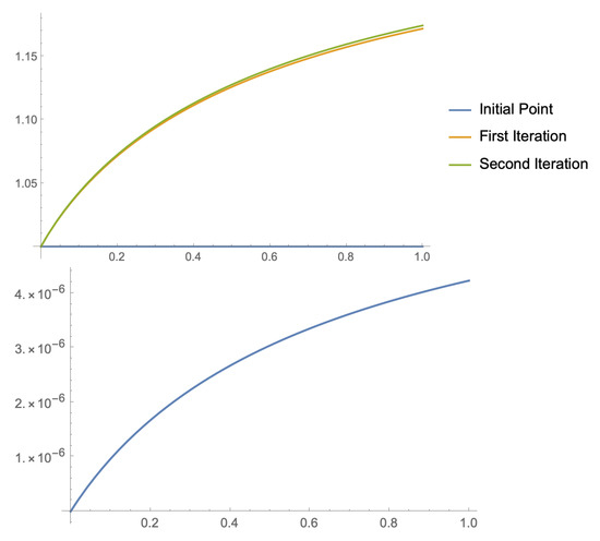
Example 1.

We consider the following Fredholm integral equation of Chandrasekhar type ([5,21]):

$$z\left(x\right)=1-\frac{1}{2}{\int }_0^1\frac{xt}{x+t}z\left(t\right)dt.$$

(20)

We take $z_0\left(x\right)=g\left(x\right)=1$ and $L_0=\mathcal{I}$ as starting points in the couple of recurrences given by (11). Let us note that, with this choice of initial guesses, the conditions of Theorem 1 are fulfilled. Actually,

$$\parallel \mathcal{I}-A{L}_0\parallel =\parallel \lambda \parallel \parallel \mathcal{N}\parallel \le \frac{1-log2}{2}\approx 0.153426$$

that is less than

$$\frac{1}{2}min\left\{\sqrt{1+\frac{4}{\left|\lambda \right|\parallel \mathcal{N}\parallel }}-1,\sqrt{5}-1\right\}=\frac{\sqrt{5}-1}{2}\approx 0.618034.$$

We would like to highlight that, in this example, we can prove the existence of a solution of Equation (20) without prior knowledge of it.

Then, taking into account the procedure explained in Section 4, we can obtain the approximated values of

$${\displaystyle z_1\left(x\right)=\sum _{j=0}^2{\lambda }^j{\mathcal{N}}^{j}g\left(x\right),z_2\left(x\right)=\sum _{j=0}^5{\lambda }^j{\mathcal{N}}^{j}g\left(x\right),}$$

and so on. In this case, we have approximated the integral operator $\mathcal{N}:\mathcal{C}[0,1]\to \mathcal{C}[0,1]$, given by

$$\mathcal{N}\left(y\right)\left(x\right)={\int }_0^1\frac{xt}{x+t}y\left(t\right)dt,$$

by using, for each $x\in [0,1]$, a Gauss–Legendre quadrature formula with four nodes and weights. We have used

$$\parallel z_n-z_{n-1}\parallel \le {10}^{-4}$$

as a stopping criterium. As we can see in Figure 1, with just a couple of iterations, we obtain a good approximation of the solution.

Figure 1. At the top, graphics of the first two iterates of Ulm’s type method (11) applied to Equation (20). In the bottom, comparison between the second and third iterations (graphic of $z_3\left(x\right)-z_2\left(x\right)$).

Example 2.

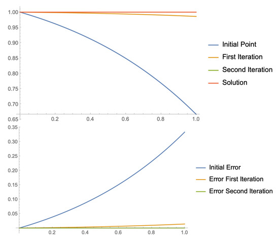
We consider now another example

$$z\left(x\right)=g\left(x\right)-\frac{1}{3}{\int }_0^{1}xt{e}^{xt}z\left(t\right)dt$$

(21)

where $g\left(x\right)$ is chosen in order to $z\left(x\right)=1$ be a solution. In this case,

$$g\left(x\right)=1-\frac{e^x(x-1)+1}{3x}ifx\ne 0;g\left(0\right)=1.$$

We take $z_0\left(x\right)=g\left(x\right)$ and $L_0=\mathcal{I}$ in (11). With this choice of initial values, the conditions of Theorem 1 are fulfilled. Actually,

$$\parallel \mathcal{I}-A{L}_0\parallel =\parallel \lambda \parallel \parallel \mathcal{N}\parallel \le \frac{1}{3}\le \frac{1}{2}min\left\{\sqrt{1+\frac{4}{\left|\lambda \right|\parallel \mathcal{N}\parallel }}-1,\sqrt{5}-1\right\}=\frac{\sqrt{5}-1}{2}\approx 0.618034.$$

Now, following the procedure explained in Section 4 and using, as in the previous example, a Gauss–Legendre quadrature formula with four nodes and weights for approximating the integral operator $\mathcal{N}:\mathcal{C}[0,1]\to \mathcal{C}[0,1]$, given by

$$\mathcal{N}\left(y\right)\left(x\right)={\int }_0^{1}xt{e}^{xt}y\left(t\right)dt,$$

we obtain, with the same stopping criterium, the approximations to the solution shown on the left side of Figure 2. In addition, as the exact solution is known, we can see the error committed by these iterations on the right side of Figure 2.

Figure 2. At the top, graphics of the first two iterates of Ulm’s type method (11) applied to Equation (21). In the bottom, graphics of the errors in these iterates.

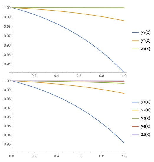
Finally, we finish with a numerical comparison between our method and Picard’s iterative method, one of the most known iterative methods for solving equations, based on a fixed point strategy. For the case of Equation (21) and starting with the same initial seed $y_0\left(x\right)=g\left(x\right)$, the following sequence of approximations to the solution can be constructed:

$$y_{n+1}\left(x\right)=g\left(x\right)-\frac{1}{3}{\int }_0^{1}xt{e}^{xt}{y}_n\left(t\right)dt,n\ge 0.$$

(22)

In Figure 3, we appreciate the faster convergence of Ulm’s type method (11) compared with Picard’s iteration (22). At the top of Figure 3, we compare the first iteration $z_1\left(x\right)$ of method (11) with two iterations $y_1\left(x\right)$ and $y_2\left(x\right)$ of Picard’s method (22). In the bottom of Figure 3, the second iteration $z_2\left(x\right)$ is compared with four iterations of Picard’s method.

Figure 3. Comparison between iterations of Ulm’s type method (11) applied to Equation (21), denoted by $z_n\left(x\right)$ and iterations of Picard’s method (22) applied to the same equation, denoted by $y_n\left(x\right)$.

6. Conclusions

We have considered the numerical solution of Fredholm integral equations of the second kind by means of iterative methods. This problem can be reduced, via the symmetry between solving linear integral equations and calculating inverse operators, to another one where it is needed to approximate the inverse of a given operator related with the integral equation. Different iterative methods can be used for this purpose, as we can see in the recent literature on this problem. For instance, Newton’s and Picard’s type methods have been used for this purpose. The use of iterative methods provides an alternative strategy for approaching this inverse and consequently the solution of the involved integral equation, instead of calculating the exact solution of the problem (see [7,9,10]).

In this paper, we have considered a variant of the well-known Ulm’s method given by (5). The choice of this method is justified by three interesting numerical properties:

• It has quadratic convergence.
• It does not contain inverse operators, or, equivalently, it is not necessary to solve a linear equation at each iteration.
• The method generates successive approximations of the inverses of the derivative at the solution, a question that is interesting to analyze the stability of the problem.

A semilocal convergence study of the method is made and a particular case of its application to a given integral Equation (1) is considered. Actually, the expression of the method for the particular initial choices $z_0\left(x\right)=g\left(x\right)$ and $L_0=\mathcal{I}$ is obtained. The paper finishes with two applications to integral equations, given by symmetric non-separable kernels.

References

- Porter, D.; Stirling, D.S.G. Integral Equations; Cambridge University Press: Cambridge, UK, 1990. [Google Scholar]
- Argyros, I.K. On a class of nonlinear integral equations arising in neutron transport. Aequationes Math. 1988, 36, 99–111. [Google Scholar] [CrossRef]
- Argyros, I.K.; Regmi, S. Undergraduate Research at Cameron University on Iterative Procedures in Banach and Other Spaces; Nova Science Publisher: New York, NY, USA, 2019. [Google Scholar]
- Bruns, D.D.; Bailey, J.E. Nonlinear feedback control for operating a nonisothermal CSTR near an unstable steady state. Chem. Eng. Sci. 1977, 32, 257–264. [Google Scholar] [CrossRef]
- Chandrasekhar, S. Radiative Transfer; Dover: New York, NY, USA, 1960. [Google Scholar]
- Davis, H.T. Introduction to Nonlinear Differential and Integral Equations; Dover: New York, NY, USA, 1962. [Google Scholar]
- Amat, S.; Ezquerro, J.A.; Hernández-Verón, M.A. Approximation of inverse operators by a new family of high-order iterative methods. Numer. Linear Algebra Appl. 2014, 21, 629–644. [Google Scholar] [CrossRef]
- Ezquerro, J.A.; Hernández-Verón, M.A. Nonlinear Fredholm integral equations and majorant functions. Numer. Algorithms 2019, 82, 1303–1323. [Google Scholar] [CrossRef]
- Gutiérrez, J.M.; Hernández-Verón, M.Á.; Martínez Molada, E. Improved iterative solution of linear Fredholm integral equations of second kind via inverse-free iterative schemes. Mathematics 2020, 8, 1747. [Google Scholar] [CrossRef]
- Hernández-Verón, M.Á.; Yadav, S.; Martínez Molada, E.; Singh, S. Solving nonlinear integral equations with non-separable kernel via a high-order iterative process. Appl. Math. Comput. 2021, 409, 126385. [Google Scholar]
- Radzuan, N.Z.F.M.; Suardi, M.N.; Sulaiman, J. KSOR iterative method with quadrature scheme for solving system of Fredholm integral equations of second kind. J. Fundam. Appl. Sci. 2017, 9, 609–623. [Google Scholar] [CrossRef][Green Version]
- Chen, Z.; Long, G.; Nelakanti, G. The Discrete Multi-Projection Method for Fredholm Integral Equations of the Second Kind. J. Int. Equation Appl. 2007, 19, 143–162. [Google Scholar] [CrossRef]
- Laurita, C.; Mastroianni, G. Condition Numbers in Numerical Methods for Fredholm Integral Equations of the Second Kind. J. Int. Equation Appl. 2002, 14, 311–341. [Google Scholar] [CrossRef]
- Sidorov, N.A.; Sidorov, D.N. Solving the Hammerstein integral equation in the irregular case by successive approximations. Sib. Math. J. 2010, 51, 325–329. [Google Scholar] [CrossRef]
- Sidorov, D.N. Existence and blow-up of Kantorovich principal continuous solutions of nonlinear integral equations. Diff. Equat. 2014, 50, 1217–1224. [Google Scholar] [CrossRef]
- Gutiérrez, J.M.; Hernández-Verón, M.Á. A Picard-Type Iterative Scheme for Fredholm Integral Equations of the Second Kind. Mathematics 2021, 9, 83. [Google Scholar] [CrossRef]
- Ulm, S. On iterative methods with successive approximation of the inverse operator (Russian). Izv. Akad Nauk Est. SSR 1967, 16, 403–411. [Google Scholar]
- Moser, J. Stable and random motions in dynamical systems with special emphasis on celestial mechanics. In Herman Weil Lectures, Annals of Mathematics Studies; Princeton University Press: Princeton, NJ, USA, 1973. [Google Scholar]
- Gutiérrez, J.M.; Hernández-Verón, M.Á.; Romero, N. A note on a modification of Moser’s method. J. Complexity 2008, 24, 185–197. [Google Scholar] [CrossRef][Green Version]
- Gutiérrez, J.M.; Hernández-Verón, M.Á. On the Convergence of Newton-Moser Method from Data at One Point. In Understanding Banach Spaces; Nova Science Publishers, Inc.: New York, NY, USA, 2019; pp. 189–198. [Google Scholar]
- Argyros, I.K. Quadratic equations and applications to Chandrasekhar’s and related equations. Bull. Austral. Math. Soc. 1985, 32, 275–292. [Google Scholar] [CrossRef]
Publisher’s Note: MDPI stays neutral with regard to jurisdictional claims in published maps and institutional affiliations. |
© 2021 by the authors. Licensee MDPI, Basel, Switzerland. This article is an open access article distributed under the terms and conditions of the Creative Commons Attribution (CC BY) license (https://creativecommons.org/licenses/by/4.0/).