On a Vector-Valued Measure of Multivariate Skewness

Abstract

The canonical skewness vector is an analytically simple function of the third-order, standardized moments of a random vector. Statistical applications of this skewness measure include semiparametric modeling, independent component analysis, model-based clustering, and multivariate normality testing. This paper investigates some properties of the canonical skewness vector with respect to representations, transformations, and norm. In particular, the paper shows its connections with tensor contraction, scalar measures of multivariate kurtosis and Mardia’s skewness, the best-known scalar measure of multivariate skewness. A simulation study empirically compares the powers of tests for multivariate normality based on the squared norm of the canonical skewness vector and on Mardia’s skewness. An example with financial data illustrates the statistical applications of the canonical skewness vector.

1. Introduction

Let $\mathbf{x}$ be a p-dimensional random vector with mean $\mathbf{\mu }$, nonsingular covariance matrix $\mathbf{\Sigma }$ and finite third-order moments. Ref. [1] introduced the vector-valued measure of multivariate skewness as follows:

$${\mathbf{\gamma }}_{1V}=\mathrm{E}\left({\mathbf{z}}^{\top }\mathbf{zz}\right),$$

where $\mathbf{z}={\mathbf{\Sigma }}^{-1/2}\left(\mathbf{x}-\mathbf{\mu }\right)$ is the standardization of $\mathbf{x}$ and ${\mathbf{\Sigma }}^{-1/2}$ is the positive definite symmetric square root of the concentration matrix ${\mathbf{\Sigma }}^{-1}$, that is, the inverse of $\mathbf{\Sigma }$:

$${\mathbf{\Sigma }}^{-1/2}>0,{\mathbf{\Sigma }}^{-1/2}={\left({\mathbf{\Sigma }}^{-1/2}\right)}^{\top },{\mathbf{\Sigma }}^{-1/2}{\mathbf{\Sigma }}^{-1/2}={\mathbf{\Sigma }}^{-1},{\mathbf{\Sigma }}^{-1/2}{\mathbf{\Sigma }\mathbf{\Sigma }}^{-1/2}={\mathbf{I}}_p.$$

The i-th element of ${\mathbf{\gamma }}_{1V}$ is as follows:

$$\mathrm{E}\left({\mathbf{z}}^{\top }\mathbf{z}{Z}_i\right)=\mathrm{E}\left(Z_1^2{Z}_i\right)+...+\mathrm{E}\left(Z_p^2{Z}_i\right),$$

where $Z_k$ is the k-th component of $\mathbf{z}$. We shall refer to ${\mathbf{\gamma }}_{1V}$ as the canonical skewness vector to distinguish it from less known vector-valued measures of multivariate skewness [2,3]. In the following, all vectors are regarded as column vectors.

The intuition behind ${\mathbf{\gamma }}_{1V}$ might be better appreciated by considering some special but relevant cases. In the univariate case, that is, when the only component of $\mathbf{x}$ is the random variable X, the skewness vector coincides with the skewness of X, that is, its third standardized moment, as follows:

$${\mathbf{\gamma }}_{1V}\left(\mathbf{x}\right)={\gamma }_1\left(X\right)=\frac{\mathrm{E}\left\{{\left(X-\mu \right)}^3\right\}}{{\sigma }^3},$$

where $\mu$ and $\sigma$ are the expected value and the standard deviation, respectively, of X. The canonical skewness vector is a null vector when $\mathbf{x}$ is centrally symmetric, that is, if $\mathbf{x}-\mathbf{\mu }$ and if $\mathbf{\mu }-\mathbf{x}$ are identically distributed [4]. In the bivariate case, the skewness vector admits the simpler representation as follows:

$${\mathbf{\gamma }}_{1V}\left(\begin{array}{c}{X}_1\\ X_2\end{array}\right)=\left(\begin{array}{c}\mathrm{E}\left(Z_1^3\right)+\mathrm{E}\left(Z_1^2{Z}_2\right)\\ \mathrm{E}\left(Z_2^3\right)+\mathrm{E}\left(Z_2^2{Z}_1\right)\end{array}\right).$$

The canonical skewness vector ${\mathbf{\gamma }}_{1V}$ appears in several areas of multivariate statistical analysis. In model-based clustering, the projection of the standardized data onto the direction of the sample counterpart of ${\mathbf{\gamma }}_{1V}$ is used to estimate the best discriminant projection [5]. In independent component analysis (ICA), ${\mathbf{\gamma }}_{1V}$ is the product of an orthogonal matrix and the vector whose i-th element is the skewness of the i-th independent component ([6]). In the semiparametric model posed by [7], ${\mathbf{\gamma }}_{1V}$ is instrumental in identifying the parameter of the model. Within an invariant coordinate selection (ICS) approach, the vector ${\mathbf{\gamma }}_{1V}$ might be regarded as the standardized difference between two appropriately chosen random vectors ([8]).

Unfortunately, the canonical skewness vector might be a null vector, even if the underlying distribution is skewed with finite third moments and a positive definite covariance matrix. For example, let the density function of the random vector $\mathbf{x}={\left(X_1,X_2,X_3\right)}^{\top }$ be $f\left(x_1,x_2,x_3;\theta \right)=2\varphi \left(x_1\right)\varphi \left(x_2\right)\varphi \left(x_3\right)\mathsf{\Phi }\left(\theta x_1{x}_2{x}_3\right)$, where $\varphi \left(·\right)$ is the standard normal probability density function, $\mathsf{\Phi }\left(·\right)$ is the standard normal cumulative distribution function, and $\theta$ is a non-null real value. Then, $\mathbf{x}$ is a standard random vector, and its only non-null third moment is $E\left(X_1{X}_2{X}_3\right)$. The canonical skewness vector is then the three-dimensional null vector.

The partial skewness ${\beta }_{1P}\left(\mathbf{x}\right)$ of $\mathbf{x}$ is just the squared norm of its canonical skewness vector:

$${\beta }_{1P}\left(\mathbf{x}\right)={∥{\mathbf{\gamma }}_{1V}\left(\mathbf{x}\right)∥}^2={\mathbf{\gamma }}_{1V}^{\top }\left(\mathbf{x}\right){\mathbf{\gamma }}_{1V}\left(\mathbf{x}\right)=\underset{i=1}{\sum ^p}\underset{h=1}{\sum ^p}\underset{k=1}{\sum ^p}\mathrm{E}\left(Z_h^2{Z}_i\right)\mathrm{E}\left(Z_k^2{Z}_i\right).$$

It was independently proposed by several authors (see, for example, refs. [1,8,9]) as a scalar measure of multivariate skewness; its name reminds that it does not depend on the cross-product moment $\mathrm{E}\left(Z_i{Z}_j{Z}_k\right)$ when i, j, and k differ from each other [6]. Partial skewness is nonnegative, equals zero if $\mathbf{x}$ is centrally symmetric, and is invariant with respect to affine, nonsingular transformations. Its statistical applications include multivariate normality testing [10] and multivariate analysis of variance [9].

Ref. [11] proposed to measure the skewness of $\mathbf{x}$ by the following expectation:

$${\beta }_{1T}\left(\mathbf{x}\right)=\mathrm{E}\left\{{\left({\mathbf{z}}^{\top }\mathbf{w}\right)}^3\right\},$$

where $\mathbf{z}$ and $\mathbf{w}$ are identically distributed and mutually independent. In the following, we shall refer to ${\beta }_{1T}$ as the total skewness since it depends on all third-order standardized moments of $\mathbf{x}$. Just like partial skewness, total skewness is nonnegative, equals zero if the underlying distribution is centrally symmetric, and is invariant with respect to nonsingular affine transformations. Moreover, just like partial skewness, total skewness is used in multivariate normality testing [11] and in multivariate analysis of variance [9]. However, ${\beta }_{1T}$ is by far more popular than ${\beta }_{1P}$, to the point of being a default measure of multivariate skewness, as remarked by [3].

The total skewness is always positive when some third-order cumulants of the underlying distribution are non-null and the covariance matrix is positive definite. This feature constitutes a major advantage of total skewness over partial skewness. For example, the total skewness and the partial skewness of the random vector $\mathbf{x}={\left(X_1,X_2,X_3\right)}^{\top }$ with probability density function $f\left(x_1,x_2,x_3;\theta \right)=2\varphi \left(x_1\right)\varphi \left(x_2\right)\varphi \left(x_3\right){\Phi }\left(\theta x_1{x}_2{x}_3\right)$ are ${\beta }_{1T}\left(\mathbf{x}\right)=6{\mathrm{E}}^2\left(X_1{X}_2{X}_3\right)$ and ${\beta }_{1P}\left(\mathbf{x}\right)=0$. As remarked before, the sample counterparts of both skewness measures were used to test normality, but they are suited for testing symmetry since there are many multivariate distributions which are centrally symmetric without being normal, such as the multivariate Student t distribution.

There are many more measures of multivariate skewness (see, for example, ref. [12]). Similarly, there are other notions of multivariate symmetry other than central symmetry, such as weak symmetry, sign symmetry and elliptical symmetry. A detailed investigation of notions of multivariate symmetry and measures of multivariate skewness falls outside the scope of the present paper. We defer the interested reader to [4], where the previous literature on both topics is thoroughly reviewed.

This paper contributes to the literature on the canonical skewness vector both with empirical and theoretical results. The theorems in Section 2 provide some alternative representations for ${\mathbf{\gamma }}_{1V}$, ${\beta }_{1P}$ and ${\beta }_{1T}$, together with some skewness–kurtosis inequalities and some insights into the behavior of these skewness measures under some well-known transformations. The simulation studies in Section 3 compare the performance of partial skewness and total skewness for testing multivariate symmetry. Section 4 uses financial data to illustrate the statistical applications of the canonical skewness vector and partial skewness. Section 5 contains some concluding remarks and hints for future research. The proofs of the theorems are relegated to Appendix A.

2. Theory

This section contains several theoretical results related to the canonical skewness vector. Theorems 1 and 2 represent the canonical skewness vector by means of the star product of matrices and the vectorization operator. Theorems 3 and 4 investigate the behavior of the canonical skewness vector under linear transformations and convolution. Theorems 5 and 6 focus on partial skewness and total skewness by providing alternative representations and by establishing skewness–kurtosis inequalities.

The third moment matrix of a p-dimensional random vector $\mathbf{x}$ with finite third-order moments is as follows:

$${\mathbf{M}}_{3,\mathbf{x}}=\mathrm{E}\left(\mathbf{x}\otimes {\mathbf{x}}^{\top }\otimes \mathbf{x}\right).$$

The matrix $\mathbf{A}\otimes \mathbf{B}$ denotes the Kronecker product of the matrices $\mathbf{A}=\left\{a_{ij}\right\}\in {\mathbb{R}}^p\times {\mathbb{R}}^q$ and $\mathbf{B}=\left\{b_{ij}\right\}\in {\mathbb{R}}^h\times {\mathbb{R}}^k$, that is, the block matrix whose $i,j$-th block is the matrix $a_{ij}\mathbf{B}.$ The third cumulant of $\mathbf{x}$, that is, the third moment of $\mathbf{x}-\mathbf{\mu }$, is the following:

$${\mathbf{K}}_{3,\mathbf{x}}={\mathbf{M}}_{3,\mathbf{x}-\mathbf{\mu }}=\mathrm{E}\left\{\left(\mathbf{x}-\mathbf{\mu }\right)\otimes {\left(\mathbf{x}-\mathbf{\mu }\right)}^{\top }\otimes \left(\mathbf{x}-\mathbf{\mu }\right)\right\}.$$

The third standardized moment of $\mathbf{x}$, which coincides with its third standardized cumulant, is the third moment (cumulant) of $\mathbf{z}$, given as follows:

$${\mathbf{K}}_{3,\mathbf{z}}={\mathbf{M}}_{3,\mathbf{z}}=\mathrm{E}\left(\mathbf{z}\otimes {\mathbf{z}}^{\top }\otimes \mathbf{z}\right).$$

The matrices ${\mathbf{M}}_{3,\mathbf{x}}$, ${\mathbf{K}}_{3,\mathbf{x}}$ and ${\mathbf{K}}_{3,\mathbf{z}}$ are the matricized versions of the third moment tensor, as follows:

$${\mathcal{M}}_{3,\mathbf{x}}=\left\{\mathrm{E}\left(X_i{X}_j{X}_h\right)\right\},$$

the third cumulant tensor, as follows:

$${\mathcal{K}}_{3,\mathbf{x}}=\left\{\mathrm{E}\left[\left(X_i-{\mu }_i\right)\left(X_j-{\mu }_j\right)\left(X_h-{\mu }_h\right)\right]\right\}$$

and the third standardized moment tensor, as follows:

$${\mathcal{M}}_{3,\mathbf{z}}=\left\{\mathrm{E}\left(Z_i{Z}_j{Z}_h\right)\right\},$$

that is, the third-order arrays containing all the third moments of $\mathbf{x}$, $\mathbf{x}-\mathbf{\mu }$, and $\mathbf{z}$. Third-order tensors provide a natural tool for representing the skewness of a random vector [1]. In particular, the canonical skewness vector is just the tensor contraction of ${\mathbf{K}}_{3,\mathbf{z}}$ and ${\mathbf{I}}_p$. Its i-th component is as follows:

$$\underset{j=1}{\sum ^p}\underset{h=1}{\sum ^p}\mathrm{E}\left(Z_i{Z}_j{Z}_h\right){\delta }_{jh},\mathrm{where}{\delta }_{jh}=\left\{\begin{array}{ccc}1& & j=h\\ & & \\ 0& & j\ne h\end{array}\right..$$

Some tensor contractions might be represented by means of the star product of matrices as defined by [13]. The star product of the $a\times b$ matrix $\mathbf{M}=\left\{m_{ij}\right\}$ and the $ac\times bd$ block matrix $\mathbf{N}=\left\{{\mathbf{N}}_{ij}\in {\mathbb{R}}^c\times {\mathbb{R}}^d\right\}$ is the $c\times d$ matrix as follows:

$$\mathbf{M}\star \mathbf{N}=\underset{i=1}{\sum ^a}\underset{j=1}{\sum ^b}{m}_{ij}{\mathbf{N}}_{ij},$$

that is, the linear combination of the blocks of $\mathbf{N}$ where the coefficients are the elements of $\mathbf{M}$. The following theorem shows that the canonical skewness vector is the star product of an identity matrix and the third standardized moment.

Theorem 1.

Let $\mathbf{z}$ be the standardization of a $\mathit{p}$-dimensional random vector $\mathbf{x}$ with a positive definite covariance matrix and finite third-order moments. Then, the canonical skewness vector ${\mathbf{\gamma }}_{1V}$ of $\mathbf{x}$ is the star product of the $p\times p$ identity matrix ${\mathbf{I}}_p$ and the third standardized cumulant matrix ${\mathbf{K}}_{3,\mathbf{z}}$:

$${\mathbf{\gamma }}_{1V}={\mathbf{I}}_p\star {\mathbf{K}}_{3,\mathbf{z}}.$$

We illustrate the above theorem with the bivariate random vector ${\left(X_1,X_2\right)}^{\top }$, whose standardization is ${\left(Z_1,Z_2\right)}^{\top }$. The star product of the $2\times 2$ identity matrix and the third standardized moment of ${\left(X_1,X_2\right)}^{\top }$ is as follows:

$$\begin{array}{c}\left(\begin{array}{cc}1& 0\\ 0& 1\end{array}\right)\star \left(\begin{array}{cc}\mathrm{E}\left(Z_1^3\right)& \mathrm{E}\left(Z_1^2{Z}_2\right)\\ \mathrm{E}\left(Z_1^2{Z}_2\right)& \mathrm{E}\left(Z_1{Z}_2^2\right)\\ \mathrm{E}\left(Z_1^2{Z}_2\right)& \mathrm{E}\left(Z_1{Z}_2^2\right)\\ \mathrm{E}\left(Z_1{Z}_2^2\right)& \mathrm{E}\left(Z_2^3\right)\end{array}\right)=1·\left(\begin{array}{c}\mathrm{E}\left(Z_1^3\right)\\ \mathrm{E}\left(Z_1^2{Z}_2\right)\end{array}\right)+\\ \\ 0·\left(\begin{array}{c}\mathrm{E}\left(Z_1^2{Z}_2\right)\\ \mathrm{E}\left(Z_1{Z}_2^2\right)\end{array}\right)+0·\left(\begin{array}{c}\mathrm{E}\left(Z_1^2{Z}_2\right)\\ \mathrm{E}\left(Z_1{Z}_2^2\right)\end{array}\right)+1·\left(\begin{array}{c}\mathrm{E}\left(Z_1{Z}_2^2\right)\\ \mathrm{E}\left(Z_2^3\right)\end{array}\right)=\\ \\ \left(\begin{array}{c}\mathrm{E}\left(Z_1^3\right)\\ \mathrm{E}\left(Z_1^2{Z}_2\right)\end{array}\right)+\left(\begin{array}{c}\mathrm{E}\left(Z_1{Z}_2^2\right)\\ \mathrm{E}\left(Z_2^3\right)\end{array}\right)=\left(\begin{array}{c}\mathrm{E}\left(Z_1^3\right)+\mathrm{E}\left(Z_1{Z}_2^2\right)\\ \mathrm{E}\left(Z_1^2{Z}_2\right)+\mathrm{E}\left(Z_2^3\right)\end{array}\right),\end{array}$$

which coincides with the canonical skewness vector of ${\left(X_1,X_2\right)}^{\top }$, as defined in the Introduction.

A location vector $\mathbf{l}\left(\mathbf{x}\right)$ and a scatter matrix $\mathbf{S}\left(\mathbf{x}\right)$ of a p-dimensional random vector $\mathbf{x}$ are a p-dimensional vector and a symmetric, positive definite $p\times p$ matrix, satisfying the following:

$$\mathbf{l}\left(\mathbf{Ax}+\mathbf{b}\right)=\mathbf{Al}\left(\mathbf{x}\right)+\mathbf{b}\mathrm{and}\mathbf{S}\left(\mathbf{Ax}+\mathbf{b}\right)=\mathbf{AS}\left(\mathbf{x}\right){\mathbf{A}}^{\top }$$

for any $p\times p$ matrix $\mathbf{A}$ of full rank and for any p-dimensional real vector $\mathbf{b}$ (see, for example, ref. [14]). The mean $\mathbf{\mu }$ and

$${\mathbf{\mu }}_{3,\mathbf{x}}=\mathrm{E}\left\{{\left(\mathbf{x}-\mathbf{\mu }\right)}^{\top }{\mathbf{\Sigma }}^{-1}\left(\mathbf{x}-\mathbf{\mu }\right)\mathbf{x}\right\}$$

are examples of location vectors [8]. The covariance and

$${\mathbf{Q}}_{\mathbf{x}}=\mathrm{E}\left\{{\left(\mathbf{x}-\mathbf{\mu }\right)}^{\top }{\mathbf{\Sigma }}^{-1}\left(\mathbf{x}-\mathbf{\mu }\right){\mathbf{xx}}^{\top }\right\}$$

are examples of scatter matrices [8]. Let ${\mathbf{l}}_1\left(\mathbf{x}\right)$, ${\mathbf{l}}_2\left(\mathbf{x}\right)$ and $\mathbf{S}\left(\mathbf{x}\right)$ be two location vectors and a scatter matrix of a p-dimensional random vector $\mathbf{x}$. Ref. [14] suggests using the following:

$${∥\mathbf{a}\left(\mathbf{x}\right)∥}^2={\left\{{\mathbf{l}}_1\left(\mathbf{x}\right)-{\mathbf{l}}_2\left(\mathbf{x}\right)\right\}}^{\top }{\mathbf{S}}^{-1}\left(\mathbf{x}\right)\left\{{\mathbf{l}}_1\left(\mathbf{x}\right)-{\mathbf{l}}_2\left(\mathbf{x}\right)\right\}$$

as a scalar measure of multivariate skewness, where ${\mathbf{S}}^{-1}\left(\mathbf{x}\right)$ is the inverse of $\mathbf{S}\left(\mathbf{x}\right)$. It measures the skewness in the direction of the vector-valued measure of multivariate skewness:

$$\mathbf{a}\left(\mathbf{x}\right)={\mathbf{S}}^{-1/2}\left(\mathbf{x}\right)\left\{{\mathbf{l}}_1\left(\mathbf{x}\right)-{\mathbf{l}}_2\left(\mathbf{x}\right)\right\},$$

where ${\mathbf{S}}^{-1/2}\left(\mathbf{x}\right)$ is the positive definite symmetric square root of ${\mathbf{S}}^{-1}\left(\mathbf{x}\right)$. The following theorem represents the canonical skewness vector and the partial skewness as $\mathbf{a}\left(\mathbf{x}\right)$ and ${∥\mathbf{a}\left(\mathbf{x}\right)∥}^2$, where the following holds:

$${\mathbf{l}}_1\left(\mathbf{x}\right)={\mathbf{\mu }}_{3,\mathbf{x}},{\mathbf{l}}_2\left(\mathbf{x}\right)=p\mathbf{\mu }\mathrm{and}\mathbf{S}\left(\mathbf{x}\right)=\mathbf{\Sigma }.$$

The theorem also represents the canonical skewness vector by means of simple matrix functions acting on the third cumulant and on the covariance matrix.

Theorem 2.

Let $\mathbf{x}$ be a p-dimensional random vector with a positive, definite covariance matrix and finite third-order moments. Additionally, let $\mathbf{\mu }$, ${\mathsf{\Sigma }}^{-1}$, and ${\mathbf{K}}_{3,\mathbf{x}}$ be the mean vector, the concentration matrix and the third cumulant of $\mathbf{x}$. Then, the canonical skewness vector of $\mathbf{x}$ is as follows:

$${\mathbf{\gamma }}_{1V}={\mathbf{\Sigma }}^{-1/2}{\mathbf{K}}_{3,\mathbf{x}}^{\top }vec\left({\mathbf{\Sigma }}^{-1}\right)={\mathbf{\Sigma }}^{-1/2}\left[\mathrm{E}\left\{{\left(\mathbf{x}-\mathbf{\mu }\right)}^{\top }{\mathbf{\Sigma }}^{-1}\left(\mathbf{x}-\mathbf{\mu }\right)\mathbf{x}\right\}-p\mathbf{\mu }\right],$$

where ${\mathbf{\Sigma }}^{-1/2}$ is the positive definite symmetric square root of ${\mathbf{\Sigma }}^{-1}$.

The canonical skewness vector is location invariant: ${\mathbf{\gamma }}_{1V}\left(\mathbf{x}\right)={\mathbf{\gamma }}_{1V}\left(\mathbf{x}+\mathbf{v}\right)$ for any p-dimensional real vector $\mathbf{v}$. On the other hand, the canonical skewness vector is neither invariant nor equivariant with respect to linear transformations: ${\mathbf{\gamma }}_{1V}\left(\mathbf{Ax}\right)$ may differ from both ${\mathbf{\gamma }}_{1V}\left(\mathbf{x}\right)$ and $\mathbf{A}{\mathbf{\gamma }}_{1V}\left(\mathbf{x}\right)$, where $\mathbf{A}$ is a nonsingular $p\times p$ real matrix. Ref. [5] conjectures that ${\mathbf{\gamma }}_{1V}\left(\mathbf{Ax}\right)=\mathbf{U}{\mathbf{\gamma }}_{1V}\left(\mathbf{x}\right)$ for some orthogonal $p\times p$ matrix $\mathbf{U}$. The following theorem makes this statement more precise.

Theorem 3.

Let ${\mathbf{\gamma }}_{1V}\left(\mathbf{x}\right)$ be the canonical skewness vector of the p-dimensional random vector $\mathbf{x}$. Additionally, let ${\mathbf{\gamma }}_{1V}\left(\mathbf{Ax}+\mathbf{b}\right)$ be the canonical skewness vector of $\mathbf{Ax}+\mathbf{b}$, where $\mathbf{A}$ is a nonsingular $p\times p$ matrix and $\mathbf{b}$ is a p-dimensional real vector. Finally, let $\mathbf{U}={\mathbf{\Sigma }}^{-1/2}{\mathbf{A}}^{-1}{\mathsf{\Omega }}^{1/2}$, where ${\mathbf{\Sigma }}^{-1/2}$ and ${\mathsf{\Omega }}^{1/2}$ are the positive definite symmetric square roots of the concentration matrix of $\mathbf{x}$ and of the covariance matrix of $\mathbf{Ax}+\mathbf{b}$. Then, $\mathbf{U}$ is orthogonal, coincides with $\mathbf{A}$ when $\mathbf{A}$ itself is orthogonal and ${\mathbf{\gamma }}_{1V}\left(\mathbf{x}\right)=\mathbf{U}{\mathbf{\gamma }}_{1V}\left(\mathbf{Ax}+\mathbf{b}\right)$.

Let $X_1$, ..., $X_n$ be independent and identically distributed random variables whose third standardized cumulant is ${\gamma }_1$. It is well-known that the third cumulant of the sum $X_1+...+X_n$ is ${\gamma }_1/\sqrt{n}$. The following theorem generalizes this statement to multivariate random vectors.

Theorem 4.

Let ${\mathbf{x}}_1$, ..., ${\mathbf{x}}_n$ be $\mathit{n}$ independent and identically distributed $\mathit{p}$-dimensional random vectors with positive definite covariance matrices and finite third-order moments. Additionally, let ${\mathbf{\gamma }}_{1V}\left({\mathbf{x}}_i\right)$, ${\beta }_{1P}\left({\mathbf{x}}_i\right)$ and ${\beta }_{1T}\left({\mathbf{x}}_i\right)$ be the canonical skewness vector, the partial skewness and the total skewness of ${\mathbf{x}}_i$, for $\mathit{i}=\mathit{1}$, ..., $\mathit{n}$. Finally, let ${\mathbf{\gamma }}_{1V}\left({\mathbf{s}}_n\right)$, ${\beta }_{1P}\left({\mathbf{s}}_n\right)$ and ${\beta }_{1T}\left({\mathbf{s}}_n\right)$ be the canonical skewness vector, the partial skewness and the total skewness of ${\mathbf{s}}_n={\mathbf{x}}_1+...+{\mathbf{x}}_n$. Then, the following identities hold true:

$${\mathbf{\gamma }}_{1V}\left({\mathbf{s}}_n\right)=\frac{{\mathbf{\gamma }}_{1V}\left({\mathbf{x}}_i\right)}{\sqrt{n}},{\beta }_{1P}\left({\mathbf{s}}_n\right)=\frac{{\beta }_{1P}\left({\mathbf{x}}_i\right)}{n}\mathrm{and}{\beta }_{1T}\left({\mathbf{s}}_n\right)=\frac{{\beta }_{1T}\left({\mathbf{x}}_i\right)}{n}.$$

The total skewness and the partial skewness are the squared norms of the third standardized moment matrix and the canonical skewness vector. Therefore, both skewness measures are functions of the third standardized moments. The following theorem shows that they can also be represented as functions of the second and third central moments, by means of simple matrix operations acting on the covariance and on the third cumulant. Thus, the following theorem provides an alternative representation for the partial and total skewness measures.

Theorem 5.

Let $\mathbf{x}$ be a p-dimensional random vector with finite third-order moments and positive definite covariance matrix. Additionally, let ${\mathbf{K}}_{3,\mathbf{x}}$ and ${\mathbf{\Sigma }}^{-1}$ be the third cumulant and the concentration matrix of $\mathbf{x}$. Then, the total skewness and the partial skewness of $\mathbf{x}$ are as follows:

$$\begin{array}{c}{\beta }_{1T}=tr\left\{{\mathbf{\Sigma }}^{-1}{\mathbf{K}}_{3,\mathbf{x}}^{\top }\left({\mathbf{\Sigma }}^{-1}\otimes {\mathbf{\Sigma }}^{-1}\right){\mathbf{K}}_{3,\mathbf{x}}\right\}\mathrm{and}\\ \\ {\beta }_{1P}=ve{c}^{\top }\left({\mathbf{\Sigma }}^{-1}\right)\left({\mathbf{K}}_{3,\mathbf{x}}{\mathbf{\Sigma }}^{-1}{\mathbf{K}}_{3,\mathbf{x}}^{\top }\right)vec\left({\mathbf{\Sigma }}^{-1}\right).\end{array}$$

The fourth-order standardized moment of a p-dimensional random vector $\mathbf{x}$ with finite fourth-order moments and positive definite covariance is as follows:

$${\mathbf{M}}_{4,\mathbf{z}}=\mathrm{E}\left(\mathbf{z}\otimes {\mathbf{z}}^{\top }\otimes \mathbf{z}\otimes {\mathbf{z}}^{\top }\right),$$

where $\mathbf{z}$ is the standardization of $\mathbf{x}$. Refs. [11,15] defined the partial kurtosis (also known as Mardia’s kurtosis) and the total kurtosis (also known as Koziol’s kurtosis) as the trace and the squared norm of the following: ${\mathbf{M}}_{4,\mathbf{z}}$:

$${\beta }_{2P}\left(\mathbf{x}\right)=tr\left({\mathbf{M}}_{4,\mathbf{z}}\right)\mathrm{and}{\beta }_{2T}\left(\mathbf{x}\right)={∥{\mathbf{M}}_{4,\mathbf{z}}∥}^2.$$

Ref. [1] as well as [16] provided some skewness–kurtosis inequalities involving partial skewness. The following theorem contributes to the literature on inequalities between multivariate measures of skewness and kurtosis.

Theorem 6.

Let $\mathbf{x}$ be a $\mathit{p}$-dimensional random vector with a positive definite covariance matrix and finite fourth-order moments. Additionally, let ${\beta }_{1T}$, ${\beta }_{1P}$, ${\beta }_{2T}$, and ${\beta }_{2P}$ be the total skewness, the partial skewness, the total kurtosis and the partial kurtosis of $\mathbf{x}$. Then, the following inequalities hold true:

$${\beta }_{1T}\le \frac{p-p^2+{\beta }_{2T}}{2}\mathrm{and}{\beta }_{1P}\le \frac{p-p^4+{\beta }_{2P}^2}{2}.$$

As a corollary, the inequality $2{\gamma }_1^2\le {\beta }_2$ holds true for a random variable X whose third and fourth standardized moments are ${\gamma }_1$ and ${\beta }_2$.

3. Simulations

In this section, we use simulations for comparing the powers of symmetry tests based on partial and total skewness. To this end, we simulated from the two-component normal mixture with proportional covariances and the multivariate skew-normal distribution. For both models, testing symmetry is a crucial issue, where ordinary likelihood-based methods are somewhat problematic. For each choice of the parameters, variables and units, we computed the percentage of samples rejected at the $0.05$ level by the testing procedure proposed by [1,11]. We refer to the former and the latter testing procedures as “Mori” and “Mardia”, respectively. The results given by the simulations clearly hint that “Mori” is a strong competitor for “Mardia”.

We first simulated 10,000 samples of 100 observations from the mixture ${\pi }_1{N}_p\left({\mathbf{0}}_p,{\mathbf{I}}_p\right)+\left(1-{\pi }_1\right)N_p\left({\mathbf{1}}_p,c·{\mathbf{I}}_p\right),$for ${\pi }_1=0.1$, $0.2$, $0.3$, $0.4$, $p=5$, 10, 15, 20 and $c=0.5$, 1, 2. The symbols ${\mathbf{0}}_p$, ${\mathbf{1}}_p$ and ${\mathbf{I}}_p$ denote the $p-$dimensional vector of zeros, the $p-$dimensional vector of ones and the $p-$dimensional identity matrix, respectively. The two-component normal mixture with proportional covariances describes the worst case from a multivariate outlier detection perspective and leads to an unbounded likelihood function (see, for example, ref. [5]). The scatter plot in Figure 1 depicts 10,000 outcomes from $0.2·N_2\left({\mathbf{0}}_2,{\mathbf{I}}_2\right)+0.8·N_2\left(2.5·{\mathbf{1}}_2,{\mathbf{I}}_2\right)$ and exemplifies the skewness of normal mixtures.

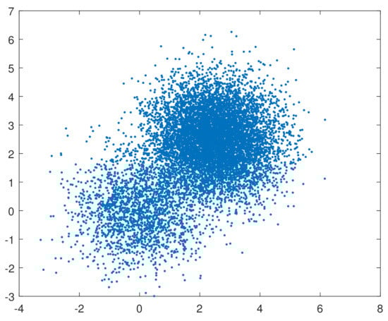
Figure 1. Scatterplot of 10,000 outcomes from $0.2·N_2\left({\mathbf{0}}_2,{\mathbf{I}}_2\right)+0.8·N_2\left(2.5·{\mathbf{1}}_2,{\mathbf{I}}_2\right)$.

The results of this simulation study are reported in Table 1 and may be summarized as follows. When less weight is placed on the more dispersed component, “Mori” always outperforms “Mardia”, although both tests show a very high power. When the components are equally dispersed, “Mardia” always outperforms “Mori”, although only slightly. Both tests show a very low power, which tends to decrease with the absolute difference between the components’ weights. When more weight is placed on the more dispersed component, “Mori” always outperforms “Mardia”, except when the weight of the less dispersed component is $0.1$. The powers of “Mardia” and “Mori” increase as $\left|2{\pi }_1-1\right|$ increases, that is, as the absolute difference between the mixture weights ${\pi }_1$ and $1-{\pi }_1$ increases.

Table 1. For samples generated from normal mixture distributions, the columns contain the percentages of samples rejected by the test based on Mardia’s skewness (header: Mardia) and by the test based on partial skewness (header: Mori) at the $0.05$ level for ${\pi }_1=0.1,0.2,0.3,0.4$, $p=5,10,15,20$ and $c=0.5,1,2$.

$\begin{array}{c}\mathit{p}\end{array}$	$\begin{array}{c}{\mathit{\pi }}_1\end{array}$	$\begin{array}{c}\mathit{c}=0.5\end{array}$	$\begin{array}{c}\mathit{c}=1\end{array}$	$\begin{array}{c}\mathit{c}=2\end{array}$
$\begin{array}{c}\mathbf{5}\end{array}$	0.1 0.2 0.3 0.4	Mardia  Mori 82.29   87.81 86.94   97.32 78.89   96.74 66.24   92.45	Mardia  Mori 10.82   9.82 7.47   7.30 5.41   4.68 3.45   3.08	Mardia  Mori 5.62   4.81 10.19   10.31 18.55   25.88 31.33   48.33
$\begin{array}{c}\\ \mathbf{10}\\ \end{array}$	0.1 0.2 0.3 0.4	Mardia  Mori 93.90   97.50 94.88   99.83 92.37   99.92 85.82   99.68	Mardia  Mori 10.83   8.64 6.11   5.23 3.79   3.11 2.63   2.10	Mardia  Mori 6.33   4.08 15.23   19.06 32.18   52.37 53.60   82.97
$\begin{array}{c}\\ \mathbf{15}\\ \end{array}$	0.1 0.2 0.3 0.4	Mardia  Mori 95.94   98.56 98.29   99.92 97.53   99.98 95.74   99.98	Mardia  Mori 7.12   4.86 3.81   2.52 2.45   1.45 1.66   0.89	Mardia  Mori 6.19   3.97 20.69   29.58 47.77   75.36 72.81   95.62
$\begin{array}{c}\\ \mathbf{20}\\ \end{array}$	0.1 0.2 0.3 0.4	Mardia  Mori 96.13   98.31 99.08   99.96 99.28   99.99 98.61   99.99	Mardia  Mori 4.10   2.08 1.88   0.91 1.17   0.47 0.78   0.33	Mardia  Mori 5.67   3.76 26.45   38.11 61.38   84.68 86.13   98.41

We also simulated 10,000 samples of sizes $n=100$, 200, 500 from the multivariate skew–normal density function $2{\varphi }_p\left(\mathbf{x};{\mathbf{0}}_p,{\mathbf{I}}_p\right)\Phi \left(\alpha {\mathbf{1}}_p^{\top }\mathbf{x}\right)$, where $\alpha =1$, 2, 3, 4 and ${\varphi }_p\left(\mathbf{x};{\mathbf{0}}_p,{\mathbf{I}}_p\right)$ is the probability density function of a p-dimensional standard normal distribution, with $p=5$, 10, 15, and 20. The information matrix of the multivariate skew–normal distribution is singular when $\alpha =0$, thus preventing the use of standard likelihood-based methods when testing symmetry. Table 2 reports the results given in this simulation study, which somewhat differ from those in the previous one. Firstly, “Mardia” nearly always outperforms “Mori”, although only slightly. Secondly, the performance of both “Mardia” and “Mori” improves with the number of units and the parameter $\alpha$, but deteriorate with the number of variables. Thirdly, the difference between the performance of “Mardia” and “Mori” tends to decrease as the number of units increases. The scatter plot in Figure 2 depicts 10,000 outcomes from $2{\varphi }_2\left(x_1,x_2;{\mathbf{0}}_2,{\mathbf{I}}_2\right)\Phi \left(2.5x_1+2.5x_2\right)$ and exemplifies the skewness of skew–normal distributions.

Table 2. For samples generated from skew–normal distributions, the columns contain the percentages of samples rejected by the test based on Mardia’s skewness (header: Mardia) and by the test based on partial skewness (header: Mori) at the $0.05$ level for $\alpha =1,2,3,4$, $p=5,10,15,20$ and $n=100,200,500$.

$\begin{array}{c}\mathit{p}\end{array}$	$\begin{array}{c}\mathit{\alpha }\end{array}$	$\begin{array}{c}\mathit{n}=100\end{array}$	$\begin{array}{c}\mathit{n}=200\end{array}$	$\begin{array}{c}\mathit{n}=500\end{array}$
$\begin{array}{c}\mathbf{5}\end{array}$	1 2 3 4	Mardia  Mori 12.58   11.59 26.67   24.97 33.46   32.24 35.99   34.40	Mardia  Mori 24.05   24.08 62.61   58.06 75.08   68.85 78.95   72.82	Mardia  Mori 67.51   62.43 99.55   97.52 99.96   99.17 99.96   99.48
$\begin{array}{c}\\ \mathbf{10}\\ \end{array}$	1 2 3 4	Mardia  Mori 6.92   5.81 10.48   9.15 11.33   10.10 11.82   10.20	Mardia  Mori 15.57   15.73 28.48   28.06 31.83   31.83 32.90   32.66	Mardia  Mori 50.83   49.70 84.04   77.13 88.89   82.61 91.34   85.02
$\begin{array}{c}\\ \mathbf{15}\\ \end{array}$	1 2 3 4	Mardia  Mori 4.17   2.45 4.88   3.04 4.94   3.19 5.38   3.22	Mardia  Mori 10.06   8.56 13.55   13.05 15.52   14.23 15.81   15.01	Mardia  Mori 33.29   34.03 51.70   51.34 57.02   55.55 58.27   56.17
$\begin{array}{c}\\ \mathbf{20}\\ \end{array}$	1 2 3 4	Mardia  Mori 2.19   0.75 2.52   1.00 2.36   1.02 2.25   0.97	Mardia  Mori 6.02   5.32 7.69   6.78 7.82   7.12 8.39   7.02	Mardia  Mori 21.27   23.43 30.64   33.01 32.63   34.13 33.89   35.27

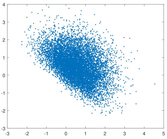
Figure 2. Scatterplot of 10,000 outcomes from $2{\varphi }_2\left(x_1,x_2;{\mathbf{0}}_2,{\mathbf{I}}_2\right)\mathsf{\Phi }\left(2.5x_1+2.5x_2\right)$.

4. Example

This section uses the financial data in [17] to illustrate a statistical application of the canonical skewness vector and the partial skewness. The dataset, which we shall refer to as ALL, includes the percentage logarithmic daily returns recorded in the French, Dutch and Spanish financial markets from 25 June 2003 to 23 June 2008. Let GOOD be the subset of ALL, which includes the returns in ALL following a positive return of the U.S. financial market, that is, good news from the leading world financial market. Similarly, let BAD be the subset of ALL, which includes all the returns in ALL following a negative return of the U.S. financial market, that is, bad news from the leading world financial market. The three datasets are instrumental in investigating the behavior of financial markets in the presence of either good or bad news [18,19].

Let $X_i$ be the i-th univariate observation in a sample of size n. The sample mean, the sample variance and the sample skewness are as follows:

$$\overline{X}=\frac{1}{n}\underset{i=1}{\sum ^n}{X}_i,S^2=\frac{1}{n}\underset{i=1}{\sum ^n}{\left(X_i-\overline{X}\right)}^2\mathrm{and}{g}_1=\frac{1}{n}\underset{i=1}{\sum ^n}{\left(\frac{X_i-\overline{X}}{S}\right)}^3.$$

The sample skewnesses of the French, Danish and Spanish data in ALL are negative: $-0.349$, $-0.236$ and $-0.461$.The sample skewnesses of the French, Danish and Spanish data in BAD are negative as well: $-0.942$, $-0.734$ and $-1.283$. On the other hand, the sample skewnesses of the French, Danish and Spanish data in GOOD are positive: $0.578$, $0.585$ and $0.774$. The absolute skewnesses of the three markets in ALL are smaller than the corresponding absolute skewnesses in GOOD, which in turn are smaller than the corresponding absolute skewnesses in BAD. All these features are well-known stylized facts of financial markets and are modeled by the SGARCH model in [18].

Let the vector ${\mathbf{x}}_i$ be the i-th multivariate observation in a sample of size n. The sample mean, the sample variance, the sample canonical skewness vector and the sample partial skewness are as follows:

$$\begin{array}{c}\overline{\mathbf{x}}=\frac{1}{n}\underset{i=1}{\sum ^n}{\mathbf{x}}_i,\mathbf{S}=\frac{1}{n}\underset{i=1}{\sum ^n}\left({\mathbf{x}}_i-\overline{\mathbf{x}}\right){\left({\mathbf{x}}_i-\overline{\mathbf{x}}\right)}^{\top },{\mathbf{z}}_i={\mathbf{S}}^{-1/2}\left({\mathbf{x}}_i-\overline{\mathbf{x}}\right),\\ \\ {\mathbf{g}}_{1V}=\frac{1}{n}\underset{i=1}{\sum ^n}{\mathbf{z}}_i^{\top }{\mathbf{z}}_i{\mathbf{z}}_i\mathrm{and}{b}_{1P}={∥{\mathbf{g}}_{1V}∥}^2=\frac{1}{n^2}\underset{i=1}{\sum ^n}\underset{j=1}{\sum ^n}{\mathbf{z}}_i^{\top }{\mathbf{z}}_i{\mathbf{z}}_j^{\top }{\mathbf{z}}_j{\mathbf{z}}_i^{\top }{\mathbf{z}}_j.\end{array}$$

In the ALL, GOOD and BAD datasets, ${\mathbf{x}}_i$ is the trivariate vector whose elements are the returns of the French, Dutch and Spanish financial markets recorded during the i-th day. The canonical skewness vectors of ALL, GOOD and BAD are negative, positive and negative:

$${\mathbf{g}}_{1V}^{ALL}=\left(\begin{array}{c}-0.359\\ -0.111\\ -0.341\end{array}\right),{\mathbf{g}}_{1V}^{GOOD}=\left(\begin{array}{c}0.275\\ 0.362\\ 0.633\end{array}\right),{\mathbf{g}}_{1V}^{BAD}=\left(\begin{array}{c}-0.771\\ -0.295\\ -1.008\end{array}\right).$$

Their squared norms, that is, the partial skewnesses of ALL, GOOD and BAD are as follows:

$$b_{1P}^{ALL}=0.258,b_{1P}^{GOOD}=0.607,b_{1P}^{BAD}=1.697.$$

The partial skewness of ALL is smaller than the partial skewness of GOOD, which in turn is smaller than the partial skewness of BAD. Therefore, for the data at hand, the canonical skewness vector and the partial skewness nicely generalize to the multivariate case and the univariate features of financial returns.

5. Conclusions

This paper investigated some theoretical and empirical properties of the canonical skewness vector. The theoretical contribution is threefold. Theorems 1 and 2 pertain to the representation of the canonical skewness vector, either with the star product or with some location vectors. Theorems 3 and 4 deal with transformations, which may be either linear transformations or convolutions. Theorems 5 and 6 highlight some connections between the partial skewness and the total skewness, with respect to representations and inequalities. The empirical contribution is twofold. Firstly, the results of the simulation studies hint that partial skewness might outperform total skewness as a test statistic for symmetry. Secondly, the canonical skewness vector, when applied to the financial data in Section 4, generalizes to multivariate financial returns—a well-known feature of univariate financial returns.

Regrettably, the literature on the analytical forms and properties of the canonical skewness vector under well-known parametric assumptions is quite sparse. For example, to the best of our knowledge, there does not exist any theoretical result regarding the canonical skewness vector of skew–elliptical distributions [20], which are very useful in modeling linear functions of order statistics (see, for example, ref. [21]). We believe that the problem might be conveniently addressed within the smaller class of scale mixtures of skew–normal distributions by jointly using the results on their moments [22,23,24] and those in this paper (see, for example, Theorem 5). Additionally, the projection of a random vector onto the direction of its canonical skewness vector has a simple parametric interpretation when the underlying distribution is a location mixture of two normal distributions with proportional covariance matrices [5]. It would be interesting to know whether this result might be somewhat extended to scale mixtures of skew–normal distributions.

For the dataset in Section 4, the canonical skewness vector and the partial skewness generalize to the multivariate case the tendency of univariate financial returns to be more skewed in the presence of bad news. This empirical result encourages addressing the following research questions. Firstly, do the results for the dataset in Section 4 hold for other financial markets and for other time periods? Secondly, could the canonical skewness vector be meaningfully used to measure the effect of news about the COVID-19 pandemic on financial markets? Thirdly, does the canonical skewness vector or the partial skewness have a simple analytical form under the multivariate SGARCH model? Fourthly, is the partial skewness of several small, capitalized financial markets smaller than the partial skewness of the same number of larger financial markets? We hope to address these interesting research questions in future works.

References

- Mòri, T.; Rohatgi, V.; Székely, G. On multivariate skewness and kurtosis. Theory Probab. Its Appl. 1993, 38, 547–551. [Google Scholar] [CrossRef]
- Balakrishnan, N.; Brito, M.; Quiroz, A. A Vectorial Notion of Skewness and Its Use in Testing for Multivariate Symmetry. Commun. Stat.-Theory Methods 2007, 36, 1757–1767. [Google Scholar] [CrossRef]
- Kollo, T. Multivariate skewness and kurtosis measures with an application in ICA. J. Multivar. Anal. 2008, 99, 2328–2338. [Google Scholar] [CrossRef]
- Serfling, R.J. Multivariate symmetry and asymmetry. In Encyclopedia of Statistical Sciences, 2nd ed.; Kotz, S., Read, C.B., Balakrishnan, N., Vidakovic, B., Eds.; Wiley: New York, NY, USA, 2006. [Google Scholar]
- Loperfido, N. Vector-Valued Skewness for Model-Based Clustering. Stat. Probab. Lett. 2015, 99, 230–237. [Google Scholar] [CrossRef]
- Loperfido, N. Singular Value Decomposition of the Third Multivariate Moment. Linear Algebra Its Appl. 2015, 473, 202–216. [Google Scholar] [CrossRef]
- Nordhausen, K.; Oja, H.; Ollila, E. Multivariate models and the first four moments. In Nonparametric Statistics and Mixture Models—A Festschrift for Thomas P. Hettmansperger; Hunter, D., Richards, D., Rosenberger, J.L., Eds.; World Scientific Publishing Co Pte Ltd.: Singapore, 2011. [Google Scholar]
- Ilmonen, P.; Oja, H.; Serfling, R. On Invariant Coordinate System (ICS) Functionals. Int. Stat. Rev. 2012, 80, 93–110. [Google Scholar] [CrossRef]
- Davis, A. On the Effects of Moderate Multivariate Nonnormality on Wilks’s Likelihood Ratio Criterion. Biometrika 1980, 67, 419–427. [Google Scholar] [CrossRef]
- Henze, N. Limit laws for multivariate skewness in the sense of Mòri, Rohatgi and Székely. Stat. Probab. Lett. 1997, 33, 299–307. [Google Scholar] [CrossRef]
- Mardia, K. Measures of multivariate skewness and kurtosis with applications. Biometrika 1970, 57, 519–530. [Google Scholar] [CrossRef]
- Malkovich, J.; Afifi, A. On Tests for Multivariate Normality. J. Am. Stat. Assoc. 1973, 68, 176–179. [Google Scholar] [CrossRef]
- MacRae, E. Matrix derivatives with an application to an adaptive linear decision problem. Ann. Stat. 1974, 2, 337–346. [Google Scholar] [CrossRef]
- Kankainen, A.; Taskinen, S.; Oja, H. Tests of multinormality based on location vectors and scatter matrices. Stat. Methods Appl. 2007, 16, 357–379. [Google Scholar] [CrossRef]
- Koziol, J. A note on measures of multivariate kurtosis. Biom. J. 1989, 31, 619–624. [Google Scholar] [CrossRef]
- Ogasawara, H. Extensions of Pearson’s inequality between skewness and kurtosis to multivariate cases. Stat. Probab. Lett. 2017, 30, 12–16. [Google Scholar] [CrossRef]
- De Luca, G.; Loperfido, N. Modelling Multivariate Skewness in Financial Returns: A SGARCH Approach. Eur. J. Financ. 2015, 21, 1113–1131. [Google Scholar] [CrossRef]
- De Luca, G.; Loperfido, N. A Skew-in-Mean GARCH Model for Financial Returns. In Skew-Elliptical Distributions and Their Applications: A Journey Beyond Normality; Genton, M.G., Ed.; Chapman & Hall, CRC: Boca Raton, FL, USA, 2004; pp. 205–222. [Google Scholar]
- De Luca, G.; Genton, M.; Loperfido, N. A Multivariate Skew-Garch Model. In Advances in Econometrics: Econometric Analysis of Economic and Financial Time Series, Part A (Special Volume in Honor of Robert Engle and Clive Granger, the 2003 Winners of the Nobel Prize in Economics); Terrell, D., Ed.; Elsevier: Oxford, UK, 2006; Volume 20, pp. 33–56. [Google Scholar]
- Branco, M.; Dey, D. A general class of skew-elliptical distributions. J. Multivar. Anal. 2001, 79, 99–113. [Google Scholar] [CrossRef]
- Loperfido, N. A Note on Skew-Elliptical Distributions and Linear Functions of Order Statistics. Stat. Probab. Lett. 2008, 78, 3184–3186. [Google Scholar] [CrossRef]
- Kim, H.M. Moments of variogram estimator for a generalized skew t distribution. J. Korean Stat. Soc. 2005, 34, 109–123. [Google Scholar]
- Kim, H.M. A note on scale mixtures of skew-normal distributions. Stat. Probab. Lett. 2008, 78, 1694–1701. [Google Scholar] [CrossRef]
- Kim, H.M. Corrigendum to “A note on scale mixtures of skew normal distribution” [Statist. Probab. Lett. 78 (2008) 1694–1701]. Stat. Probab. Lett. 2013, 83, 1937. [Google Scholar] [CrossRef]
- Rao, C.; Rao, M. Matrix Algebra and Its Applications to Statistics and Econometrics; World Scientific Co. Pte. Ltd.: Singapore, 1998. [Google Scholar]
- Kollo, T.; Srivastava, M. Estimation and testing of parameters in multivariate Laplace distribution. Commun. Stat.-Theory Methods 2005, 33, 2363–2687. [Google Scholar] [CrossRef]
- Kotz, S.; Balakrishnan, N.; Johnson, N. Continuous Multivariate Distributions, Volume 1: Models and Applications, 2nd ed.; Wiley: New York, NY, USA, 2000. [Google Scholar]
Publisher’s Note: MDPI stays neutral with regard to jurisdictional claims in published maps and institutional affiliations. |
© 2021 by the author. Licensee MDPI, Basel, Switzerland. This article is an open access article distributed under the terms and conditions of the Creative Commons Attribution (CC BY) license (https://creativecommons.org/licenses/by/4.0/).