Behavior of the Eigenvalues and Eignfunctions of the Regge-Type Problem

Abstract

This article investigates the spectral theory of the problem of the Regge-type with transmission conditions and discontinuous coefficients. We formulate a new linear operator, by which we can deal with simplicity and boundedness of the eigenpairs of the problem. The aim of this work is to conduct that the problem has an infinite number of simple positive eigenvalues.

1. Introduction

A variety of scholars have studied the process of seeking eigen-pairs of the topic of spectral problem. Naimark [1] examined the general linear differential operator of nth order. He has derived an approximate formula for fundamental solutions, eigen-pairs to the problem. Eventually, a second order differential operator was investigated by Kerimov and Mamedov [2]. They have obtained valid approximate formulas for self-value and self-function. The Regge problem arises in the development of quantum scattering when the potential is present a finite support for interaction. The S-wave radial Schrödinger equation in physics, which occurs after separation of variables in the three-dimensional Schrödinger equation with radial symmetric potential, is just the Sturm–Liouville equation on the semiaxis (for more details about Regge problem, see Reference [3]):

$$-y^{{}^{″}}(x,\lambda )+q\left(x\right)y(x,\lambda )={\lambda }^{2}y(x,\lambda ).$$

(1)

At $x=0$, the boundary condition is:

$$y(0,\lambda )=0.$$

(2)

Although the type of interaction in nuclear physics is unclear, various models have been suggested. Regge’s assertion was that the potential has finite support, for a positive number a, then boundary condition is:

$$y^{{}^{\prime }}(a,\lambda )+i\lambda y(a,\lambda )=0,$$

(3)

Móller and Pivovarchik [4] claimed the quantum mechanics problem that $q\left(x\right)\in L^2(0,a)$ must be real. It should be observed that different authors look for different classes of potentials, e.g., $L^1(0,a)$ or $C(0,a)$. The problem (1)–(3) on $L^2(0,a)$ is referred to the Regge problem.

Lately, the investigation of the problem of finding eigenvalue has the line of discontinuity on the solutions or coefficients of the differential operator [5,6,7,8,9]. In their article [10], Yang and Wang studied the class of Sturm–Liouville operators with their spectral parameter-dependent boundary conditions and transmission conditions at finite interior points. By manipulating the inner product in the appropriate Krein space associated with the problem, a new self-adjoint operator is generated in such a way that the eigenvalues of such a problem correspond with those of the operator, for more information on about linear operators in Hilbert and Krein spaces, we recommend reference [11]. Many authors work on Regge-type problems for different cases [12,13,14], but there is no specific working for the Regge problem with transmission conditions. Stimulated by Reference [15], we examine the problem of the Regge-type with transmission conditions and discontinuous coefficient. In this paper, we analyze the spectral properties and the approximate properties of the problem. Next, we construct the problem as follows:

$$L\left[y\right]=-y^{{}^{″}}(x,\lambda )+q\left(x\right)y(x,\lambda )=\lambda y(x,\lambda )$$

(4)

on the interval $[0,r)\cup (r,a]$, where a is a positive real number, and $0<r<a$, with the boundary condition at $x=0$:

$$L_1\left[y\right]=y(0,\lambda )=0,$$

(5)

with the transmission conditions at $x=r$:

$$L_2\left[y\right]=y(r+,\lambda )-y(r-,\lambda )+\lambda {\delta }_1{y}^{{}^{\prime }}(r-,\lambda )=0,$$

(6)

$$L_3\left[y\right]=y^{{}^{\prime }}(r+,\lambda )-y{}^{\prime }(r-,\lambda )+\lambda {\delta }_{2}y(r-,\lambda )=0,$$

(7)

and the boundary condition at $x=a$:

$$L_4\left[y\right]=y^{{}^{\prime }}(a,\lambda )+i\lambda y(a,\lambda )=0,$$

(8)

where $\lambda$ is the complex spectral parameter; ${\delta }_1$, ${\delta }_2$ are real constants with $|{\delta }_1|+|{\delta }_2|\ne 0$, and $q\left(x\right)$ is a discontinuous function defined on $[0,r)\cup (r,a]$ as follows:

$$q\left(x\right)=\left\{\begin{array}{cc}{q}_1\left(x\right);\hfill & x\in [0,r)\hfill \\ q_1\left(x\right);\hfill & x\in (r,a].\hfill \end{array}\right.$$

(9)

The functions $q_1\left(x\right)$, $q_2\left(x\right)$ are continuous on the interval $[0,r)$, $(r,a]$, respectively, $q_1\in C^2[0,r)$, $q_2\in C^2(r,a]$, and they have finite limits, $q_1(r\pm )={lim}_{x\to r\pm }{q}_1\left(x\right)$, $q_2(r\pm )={lim}_{x\to r\pm }{q}_2\left(x\right)$.

This work is structured as follows: Firstly, we give some preliminaries on problem’s converted linear operator. In Section 3, we are focused on estimating formulas for linearly independent solutions of (4). We also measure the upper limit for the solution. The last part of this paper is devoted to formulate the approximate formulas for the eigen-pairs of problems (4)–(8). As for Theorem 4, the problem (4)–(8) has an infinite number of eigenvalues. Theorem 5 has then shown that the zeros of $W_1\left(\lambda \right)$ are the peculiar values of the query.

2. The Operator Formulation for the Problem

In this section, we investigate the properties of the Regge-type problem (4)–(8) in terms of a linear operator U that introduced in a special Hilbert space $H:=L^2\left((0,r)\cup (r,a)\right)\oplus \mathbb{C}\oplus {\mathbb{C}}_{{\delta }_1}\oplus {\mathbb{C}}_{{\delta }_2}$. First of all, we reconstruct an inner product $⟨.,.⟩$ in the linear space H. The linear operator U is defined by means of this inner product $⟨.,.⟩$. As a special case, the problem (4)–(8) can be rewritten as the spectral problem for U. To begin with, we introduce the inner product ${⟨.,.⟩}_1$ on $L^2\left((0,r)\cup (r,a)\right)$, for any $f,g\in L^2\left((0,r)\cup (r,a)\right)$ as follows:

$${⟨f,g⟩}_1={\int }_0^r{f}_1\overline{g_1}dx+{\int }_r^a{\overline{f}}_2{g}_{2}dx,$$

(10)

where $f_1{=f\left(x\right)|}_{[0,r)}$, and $f_2{=f\left(x\right)|}_{(r,a]}$. It is easy to show that $(L^2\left((0,r)\cup (r,a)\right),{⟨·⟩}_1)$ form a Hilbert space. Suppose that $[.,.]$ is defined in H as:

$$[F,G]={⟨f,g⟩}_1+⟨h_1,k_1⟩+⟨h_2,k_2⟩+⟨h_3,k_3⟩,$$

(11)

for any $F=(f,h_1,h_2,h_3)$ and $G=(g,k_1,k_2,k_3)$ in the space H. Now, the inner product $(.,.)$ defined by means of $[.,.]$ as:

$$(f,g)=[Jf,g],$$

where J is the fundamental symmetry of the Krein space H. Now, we want to formulate the process of finding the eigenvalues of problem (4)–(8). This method has been studied by many authors [6,7,8,16,17]: If $J_0:L^2\left(I\right)\to L^2\left(I\right)$ is defined by $\left(J_{0}f\right)\left(x\right)=f\left(x\right)$, then

$$J=\left[\begin{array}{cccc}{J}_0& 0& 0& 0\\ 0& 1& 0& 0\\ 0& 0& sgn{\delta }_1& 0\\ 0& 0& 0& sgn{\delta }_2\end{array}\right].$$

It is clear that $⟨.,.⟩=[J.,.]$ is a positive definite on H. This means that H is a Hilbert space with the inner product $⟨.⟩=[J.,.]$ as specified by $H_0:=(H,⟨.,.⟩)$. Let U be a linear operator defined according to the conditions of our problem (4)–(8):

$$\begin{array}{cc}\hfill D\left(U\right):=\{& (f,h_1,h_2,h_3)\in H|f_1^{\left(i\right)}\in A{C}_{loc}\left((0,r)\right),f_2^{\left(i\right)}\in A{C}_{loc}\left((r,a)\right),i=1,2,\hfill \\ & Lf\in L^2\left((0,r)\cup (r,a)\right),L_{k}f=0,k=1,2,h_1=-{\delta }_1{f}^{{}^{\prime }}\left(r\right),h_2=-{\delta }_{2}f\left(r\right),\hfill \\ & h_3=if\left(a\right)\}\hfill \end{array}$$

Then, for any $F=(f,-{\delta }_1{f}^{{}^{\prime }}\left(r\right),-{\delta }_{2}f\left(r\right),if\left(a\right))\in D\left(A\right)$, we have

$$UF=(Lf,f(r+)-f(r-),f^{{}^{\prime }}(r+)-f^{{}^{\prime }}(r-),f^{{}^{\prime }}\left(a\right)).$$

(12)

Hence, we can represent problem (4)–(8) in the following form:

$$UF=\lambda F.$$

Note that the eigenvalues of the Regge-type problem (4)–(8) and the linear operator U defined on H are the same. This allows one to address the problem in the direction of operator theory. We will interact with the properties of this operator at a higher stage in the Krein or Hilbert spaces. The G subset of the normalized linear space X is said to be dense in X, if each element x of G is the limit for the series in X. In the following Theorem, we analyze the domain density of the operator U, which was established in $H0$ due to problem (4)–(8). As a consequence, we show that U is self-adjoint in $H_0$.

Theorem 1.

The linear operator U, that is defined in (12), is densely defined in the Hilbert space $H_0$.

Proof. 

If $\varphi \left(x\right)$ is introduced as:

$$\varphi \left(x\right)=\left\{\begin{array}{cc}{\varphi }_1\left(x\right):\hfill & x\in [0,r)\hfill \\ {\varphi }_2\left(x\right):\hfill & x\in (r,a]\hfill \end{array}\right.,$$

(13)

where ${\varphi }_1\left(x\right)\in C^{\infty }(0,r)$ and ${\varphi }_2\left(x\right)\in C^{\infty }(r,a)$. If W is the set of all functions of the form $\varphi \left(x\right)$, then W is dense in $H_0$, (see Reference [16], Lemma 2.1). Hence, $D\left(U\right)$ is dense set in $H_0$. □

Theorem 2.

The operator U, defined in (12), is self-adjoint in $H_0$.

Proof. 

The proof is similar to Reference [16], Theorem 2.2. □

Let A be a linear map on a subspace of a Hilbert space H, which it is known as the “domain” of A. We assume that $Dom\left(A\right)$ is a dense subspace of H. Then, A is said to be symmetric if

$$⟨Ax,y⟩=⟨x,Ay⟩$$

for all elements x and y in $D\left(A\right)$.

Theorem 3.

The linear operator U, that is defined in (12), is symmetric in the Hilbert space $H_0$.

Proof. 

It is similar to Reference [15], Theorem 2.2. □

Theorem 4.

The set of eigenvalues of the operator U, that is defined in (12), containing infinity positive eigenvalues.

Proof. 

For the proof, see Reference [18], Proposition 1.8. □

Lemma 1.

For any $\lambda \in \mathbb{C}$ and $b\in [0,r)\cup (r,a]$, the differential equation

$$y^{{}^{″}}(x,\lambda )+q_i\left(x\right)y(x,\lambda )=\lambda y(x,\lambda ),fori=1,2$$

has a unique solution, which satisfies the initial conditions

$$y(b,\lambda )=C_1\left(\lambda \right),y^{{}^{\prime }}(b,\lambda )=C_2\left(\lambda \right),$$

where $q_1\left(x\right)$, $q_2\left(x\right)$ are continuous functions on the interval $[0,r)$, $(r,a]$, respectively, defined in (9) and $C_i\left(\lambda \right)$, (for $i=1,2$) are entirely on $\mathbb{C}$.

Proof. 

When the functions $q_1\left(x\right)$ and $q_2\left(x\right)$ are continuous functions on the domain $[0,r)$, $(r,a]$, respectively, the proof is obtained directly by using the Existence and Uniqueness Theorem. □

Because $b=0$, therefore, the solution ${\xi }_{11}(x,\lambda )$ of the differential Equation (4) on $[0,r)$ occurs by Lemma 1, such that the initial conditions were met.

$$\begin{array}{c}\hfill {\xi }_{11}\left(0\right)=0,{\xi }_{11}^{{}^{\prime }}\left(0\right)=-1.\end{array}$$

(14)

Owing to this solution, we take another solution ${\xi }_{12}(x,\lambda )$ of the differential Equation (4) at the interval $(r,a]$, so that the initial conditions at $a=r$ are fulfilled.

$$\begin{array}{c}\hfill {\xi }_{12}\left(r\right)={\xi }_{11}\left(r\right)-\lambda {\delta }_1{\xi }_{11}^{{}^{\prime }}\left(r\right),{\xi }_{12}^{{}^{\prime }}\left(r\right)={\xi }_{11}^{{}^{\prime }}\left(r\right)-\lambda {\delta }_2{\xi }_{11}\left(r\right).\end{array}$$

(15)

Hence,

$$u(x,\lambda )=\left\{\begin{array}{cc}{\xi }_{11}(x,\lambda );\hfill & x\in [0,r)\hfill \\ {\xi }_{12}(x,\lambda );\hfill & x\in (r,a]\hfill \end{array}\right.$$

(16)

is a linearly independent solution for the differential Equation (4) on the interval $[0,r)$, $(r,a]$. Finally, we have to find another linearly independent solution to measure the formula for the problem pairs (4)–(8). Again, using Lemma 1, Equation (4) has two solutions: ${\varphi }_{21}(x,\lambda )$ and ${\varphi }_{22}(x,\lambda )$ on the intervals $[0,r)$ and $(r,a]$, respectively.

$$\begin{array}{c}\hfill \left\{\begin{array}{cc}{\varphi }_{22}\left(a\right)=-1,{\varphi }_{22}^{{}^{\prime }}\left(a\right)=i\lambda \hfill & \\ {\varphi }_{21}\left(r\right)={\varphi }_{22}\left(r\right)+\lambda {\delta }_1{\varphi }_{22}^{{}^{\prime }}\left(r\right),{\varphi }_{21}^{{}^{\prime }}\left(r\right)={\varphi }_{22}^{{}^{\prime }}\left(r\right)+\lambda {\delta }_2{\varphi }_{22}\left(r\right)\hfill \end{array}\right..\end{array}$$

(17)

This means that the function $v(x,\lambda )$ forms a linearly independent solution for (4) on the interval $[0,r)$, $(r,a]$, where:

$$v(x,\lambda )=\left\{\begin{array}{cc}{\varphi }_{21}(x,\lambda );\hfill & x\in [0,r)\hfill \\ {\varphi }_{22}(x,\lambda );\hfill & x\in (r,a]\hfill \end{array}\right..$$

(18)

Consider the linear differential operator:

$$L\left[y\right]=y^{\left(2\right)}\left(x\right)+q\left(x\right)y=\lambda \omega \left(x\right)y(x,\lambda ).$$

The above differential equation has a fundumental system of 2 linearly independent solutions $y_1,y_2$ at the interval $[a,b]\subseteq \mathbb{R}$ [19]. If we have the following boundary conditions $L_i{\left[y\right]}_{a,b}={\alpha }_i$, for $i=1,2$, then the problem’s eigenvalues are the roots of the equation:

$$\left|\begin{array}{cc}{L}_1\left[y_1\right]& L_1\left[y_2\right]\\ L_2\left[y_1\right]& L_2\left[y_2\right]\end{array}\right|=0.$$

(19)

From the boundary conditions (5)–(8) and Equation (19), we provide the following Wronskians:

$$W_1\left(\lambda \right)=\left|\begin{array}{cc}{\xi }_{11}(x,\lambda )& {\varphi }_{21}(x,\lambda )\\ {\xi }_{11}^{{}^{\prime }}(x,\lambda )& {\varphi }_{21}^{{}^{\prime }}(x,\lambda )\end{array}\right|,$$

(20)

and

$$W_2\left(\lambda \right)=\left|\begin{array}{cc}{\xi }_{12}(x,\lambda )& {\varphi }_{22}(x,\lambda )\\ {\xi }_{12}^{{}^{\prime }}(x,\lambda )& {\varphi }_{22}^{{}^{\prime }}(x,\lambda )\end{array}\right|.$$

(21)

The Wronskians are equivalent. That is, $W_1\left(\lambda \right)=W_2\left(\lambda \right)$, for $\lambda \in \mathbb{C}$. Hence, (19)–(21) imply the following significant properties for obtaining a formula to establish the eigenvalues of problem (4)–(8):

Theorem 5.

The eigenvalues the problem of (4)–(8) are the roots of the characteristic equations $W_1\left(\lambda \right)=W_2\left(\lambda \right)$.

Theorem 6.

The problem (4)–(8) has only simple eigenvalues.

Proof. 

See the last note of Section 4. □

3. Construction of the Fundamental Solutions

This section focuses on calculating formulas for linearly independent solutions of (4) such that each solution meets the initial conditions (14)–(17), respectively. We also measure the upper limit for the solution.

Lemma 2.

Let $\lambda =s^2,s=\sigma +i\tau$. Then, the fundamental solution (16) (respectively, its derivative) satisfy the following integral equations:

$$\begin{array}{c}\hfill {\xi }_{11}(x,\lambda )=\frac{-1}{s}sin\left(sx\right)-\frac{1}{s}{\int }_0^{x}sin\left(s(x-t)\right)q_1\left(t\right){\xi }_{11}\left(t\right)dt,\end{array}$$

(22)

$$\begin{array}{c}\hfill {\xi }_{11}^{{}^{\prime }}(x,\lambda )=-cos\left(sx\right)-{\int }_0^{x}cos\left(s(x-t)\right)q_1\left(t\right){\xi }_{11}\left(t\right)dt,\end{array}$$

(23)

$$\begin{array}{cc}\hfill {\xi }_{12}(x,\lambda )& =\left[\frac{1}{s}{\xi }_{11}^{{}^{\prime }}\left(r\right)-s{\delta }_2{\xi }_{11}\left(r\right)\right]sin\left(s(x-r)\right)+\left[{\xi }_{11}\left(r\right)-s^2{\delta }_1{\xi }_{11}^{{}^{\prime }}\left(r\right)\right]cos\left(s(x-r)\right)\hfill \\ & -\frac{1}{s}{\int }_r^{x}sin\left(s(x-t)\right)q_2\left(t\right){\xi }_{12}\left(t\right)dt,\hfill \end{array}$$

(24)

$$\begin{array}{cc}\hfill {\xi }_{12}^{{}^{\prime }}(x,\lambda )& =\left[{\xi }_{11}^{{}^{\prime }}\left(r\right)-s^2{\delta }_2{\xi }_{11}\left(r\right)\right]cos\left(s(x-r)\right)+\left[s{\xi }_{11}\left(r\right)-s^3{\delta }_1{\xi }_{11}^{{}^{\prime }}\left(r\right)\right]sin\left(s(x-r)\right)\hfill \\ & -{\int }_r^{x}cos\left(s(x-t)\right)q_2\left(t\right){\xi }_{12}\left(t\right)dt.\hfill \end{array}$$

(25)

Proof. 

Remember Equation (4), so that we can now reform it as follows:

$$y^{{}^{″}}(x,\lambda )+s^{2}y(x,\lambda )=m\left(x\right).$$

(26)

Assuming $m\left(x\right)=q_1\left(x\right)y(x,\lambda )$, therefore, expression (26) has an unique linearly independent solution ${\xi }_{11}(x,\lambda )$ on $[0,r)$, which passes the initial condition (14) of Lemma 1. It is simple to confirm that $e^{isx}$, and $e^{-isx}$ are linearly independent solutions:

$$y^{{}^{\prime }}(x,\lambda )-s^{2}y(x,\lambda )=0.$$

Using the Parameter Variance process, the solution ${\xi }_{11}(x,\lambda )$ has the following form:

$$\begin{array}{c}\hfill {\xi }_{11}(x,\lambda )=\frac{-1}{s}sin\left(sx\right)-\frac{1}{s}{\int }_0^{x}sin\left(s(x-t)\right)q_1\left(t\right){\xi }_{11}\left(t\right)dt.\end{array}$$

Thus, we acquire (22). By applying the Lebintz law, we differentiate this integral inequality with respect to x, and then we obtain (23). Using related arguments, we get (24) and (25). □

Lemma 3.

Let $\lambda =s^2,s=\sigma +i\tau$. Then, for a sufficiently large value of $\left|\lambda \right|$, the fundamental solution (16) (respectively, its derivative) has the following approximate formulas:

$$\begin{array}{c}\hfill {\xi }_{11}(x,\lambda )=\frac{-1}{s}sin\left(sx\right)+O\left(\frac{1}{{\left|s\right|}^2}{e}^{\left|s\right|x}\right),\end{array}$$

(27)

$$\begin{array}{c}\hfill {\xi }_{11}^{{}^{\prime }}(x,\lambda )=-cos\left(sx\right)+O\left(\frac{1}{\left|s\right|}{e}^{\left|s\right|x}\right),\end{array}$$

(28)

$$\begin{array}{c}\hfill {\xi }_{12}(x,\lambda )=-s^2{\delta }_1{\xi }_{11}^{{}^{\prime }}\left(r\right)cos\left(s(x-r)\right)+O\left(\left|s\right|e^{\left|s\right|x}\right),\end{array}$$

(29)

$$\begin{array}{c}\hfill {\xi }_{12}^{{}^{\prime }}(x,\lambda )=s^3{\delta }_1{\xi }_{11}^{{}^{\prime }}\left(r\right)sin\left(s(x-r)\right)+O\left({\left|s\right|}^2{e}^{\left|s\right|x}\right).\end{array}$$

(30)

Proof. 

Suppose that $F_{11}(x,\lambda )=\left|s\right|e^{-\left|s\right|x}{\xi }_{11}(x,\lambda )$, and $M=ma{x}_{x\in [0,r)}\left|F_{11}(x,\lambda )\right|$; then, we have the following inequality for $F_{11}(x,\lambda )$:

$$|F_{11}(x,\lambda )|\le 1+M{\int }_0^x|q_1\left(t\right)dt.$$

Since $q_1\left(t\right)$ is continuous on $[0,r)$, then ${\int }_0^x|q_1\left(t\right)dt$ is bounded, which implies that $F_{11}(x,\lambda )=O\left(1\right)$. Hence, we have ${\xi }_{11}=O\left(\frac{1}{\left|s\right|}{e}^{\left|s\right|x}\right)$. By substituting this value in (22), then the approximate formula (27) holds. Similarly, we obtain (28), by differentiating (23) with respect to x. If $x=r$ in the integral Equation (22), then

$$\begin{array}{c}\hfill {\xi }_{11}(r,\lambda )=\frac{-1}{s}sin\left(sr\right)-\frac{1}{s}{\int }_0^{r}sin\left(s(r-t)\right)q_1\left(t\right){\xi }_{11}\left(t\right)dt,\end{array}$$

(31)

$$\begin{array}{c}\hfill {\xi }_{11}^{{}^{\prime }}(r,\lambda )=-cos\left(sr\right)-{\int }_0^{r}cos\left(s(r-t)\right)q_1\left(t\right){\xi }_{11}\left(t\right)dt.\end{array}$$

(32)

Substituting (31), (32) in (29), putting $F_{12}(x,\lambda )={\left|s\right|}^{-2}{e}^{-\left|s\right|x}{\xi }_{12}(x,\lambda )$ and $M_1=ma{x}_{x\in [0,r)}\left|F_{11}(x,\lambda )\right|$, we obtain the following inequality for $F_{12}(x,\lambda )$:

$$|F_{12}(x,\lambda )|\le \frac{2}{{\left|s\right|}^3}+\frac{{\delta }_2}{{\left|s\right|}^2}+\frac{M_1}{\left|s\right|}{\int }_r^x|q\left(t\right)dt+M_0,$$

for some $M_0>0$, which implies that $F_{12}(x,\lambda )=O\left(1\right)$. Hence, we have ${\xi }_{12}=O\left({\left|s\right|}^2{e}^{\left|s\right|x}\right)$. By substituting this value in (24), then the approximate formula (29) holds. Similarly, we obtain (30), by differentiating (25) with respect to x. □

During the next Lemma, we set the approximate formula for the linearly independent solution $v(x,\lambda )$.

Lemma 4.

Let $\lambda =s^2,s=\sigma +i\tau$. Then, for a sufficiently large value of $\left|\lambda \right|$, the fundamental solution (18) (respectively, its derivative) has the following approximate formulas:

$$\begin{array}{c}\hfill {\varphi }_{22}(x,\lambda )=issin\left(s(x-a)\right)+O\left(e^{\left|s\right|(a-x)}\right),\end{array}$$

(33)

$$\begin{array}{c}\hfill {\varphi }_{22}^{{}^{\prime }}(x,\lambda )=-i{s}^{2}cos\left(s(x-a)\right)+O\left(\left|s\right|e^{\left|s\right|(a-x)}\right),\end{array}$$

(34)

$$\begin{array}{c}\hfill {\varphi }_{21}(x,\lambda )=-s^2{\delta }_1{\varphi }_{22}^{{}^{\prime }}\left(r\right)cos\left(s(x-r)\right)+O\left({\left|s\right|}^3{e}^{\left|s\right|(a-x)}\right),\end{array}$$

(35)

$$\begin{array}{c}\hfill {\varphi }_{21}^{{}^{\prime }}(x,\lambda )=s^3{\delta }_1{\varphi }_{22}^{{}^{\prime }}\left(r\right)sin\left(s(x-r)\right)+O\left({\left|s\right|}^4{e}^{\left|s\right|(a-x)}\right).\end{array}$$

(36)

Proof. 

It is similar to Lemma 3. □

Next, we are inspired to approximate the upper limits for the solutions of the problem under certain thought. First of all, from Equation (22):

$$\begin{array}{c}\hfill {\xi }_{11}(x,\lambda )=\frac{-1}{s}sin\left(sx\right)-\frac{1}{s}{\int }_0^{x}sin\left(s(x-t)\right)q_1\left(t\right){\xi }_{11}\left(t\right)dt,\end{array}$$

consider $s=\sigma +i\tau$, $M={\max }_{x\in \left[0,r\right)}{e}^{\left|w_1\left(x+1\right)\right|}$, $Q_1\left(t\right)={max}_{t\in [0,r)}\left\{\right|q_1\left(t\right)\left|\right\}$,${\int }_0^x\left|Q\left(t\right)\right|dt<\infty$ and $\left|\tau \right|\le \left|\sigma \right|$. Then, the following relations $\left|\sin z\right|\le e^{\left|Imz\right|}$ and $\left|\cos z\right|\le e^{\left|Imz\right|}$, imply the following inequalities: $\left|\sin s\left(x\right)\right|\le M^{\left|\tau \right|}\le M^{\left|\sigma \right|}$. Hence, we obtain an upper bound for the solution (16):

$$\left|{\xi }_{11}\right|\le M^{\left|\sigma \right|}{C}_1{e}^{C_2},$$

for $C_2={\int }_0^x\left|Q\left(t\right)\right|dt$ and $C_1=\frac{1}{\left|s\right|}$. In the same way as above, we can estimate upper bounds for Equations (23)–(30). Hence, we have the following result:

Theorem 7.

The spectrum λ is eigenvalue for problem (4)–(8), for all $\lambda >0$, where the following conditions were occurred

$$\underset{x\in \left[0,r\right)\cup (r,a]}{\sup }u(x,\lambda )={\xi }_0<\infty ,$$

$${\int }_0^x\left|q_1\left(t\right)\right|dt<\infty and{\int }_x^a\left|q_2\left(t\right)\right|dt<\infty .$$

Proof. 

Since the linearly independent solutions are bounded, the proof is similar to Reference [8], Theorem 2.1. □

4. Approximate Formulas for the Egenvalues and Eigenfunctions of Problem (4)–(8)

For this part, we create the necessary approximate formulas for the eigen-pairs of problems (4)–(8). As for Theorem 4, the problem (4)–(8) has an infinite number of eigenvalues. Theorem 5 has then shown that the zeros of $W_1\left(\lambda \right)$ are the peculiar values of the query. So, again, we need to calculate the expression for $W_1\left(\lambda \right)$:

Theorem 8.

Suppose that $\lambda =s^2,s=\sigma +i\tau$. Then, $W_1\left(\lambda \right)$ has the following expression form:

$$\begin{array}{c}\hfill W_1\left(\lambda \right)=-s^4{\delta }_{1}cos\left(s\left(r\right)\right)cos\left(s(r-a)\right)+O\left({\left|s\right|}^3{e}^{2\left|s\right|\left(a\right)}\right),\end{array}$$

(37)

for a sufficiently large $\left|\lambda \right|$.

Proof. 

Because the functions ${\xi }_{11}(x,\lambda )$ meet the initial conditions (14) and ${\varphi }_{22}(x,\lambda )$ meet the boundary conditions (8), then (29), (30), and (20), we derive the following expression:

$$W_1\left(\lambda \right)=\left|\begin{array}{cc}0& {\varphi }_{21}(0,\lambda )\\ -1& {\varphi }_{21}^{{}^{\prime }}(0,\lambda )\end{array}\right|={\varphi }_{21}(0,\lambda )=-s^2{\delta }_1{\varphi }_{22}^{{}^{\prime }}\left(r\right)cos\left(s\left(r\right)\right)+O\left({\left|s\right|}^3{e}^{2\left|s\right|\left(a\right)}\right).$$

(38)

If you evaluate ${\varphi }_{22}^{{}^{\prime }}(r,\lambda )$ and overwrite it with Equation (38), then you get (37). By a related argument, we can obtain the same approximation for the characteristic $W_2\left(\lambda \right)$ equation. □

Mind that, if $\lambda$ is a negative real number, say $\lambda =-t^2$, then we can logically argue that $W1(-t^2)\to \infty$ has a large value of t. Such an element means that the eigenvalues of problem (4)–(8) are bounded below, so that we can conclude that the eigenvalues are

$$\lambda 0\le \lambda 1\le \lambda 2\le \lambda 3\le \dots$$

throughout the manner of an increasing sequence. In the next theorem, we describe the approximate formula for the eigenvalues:

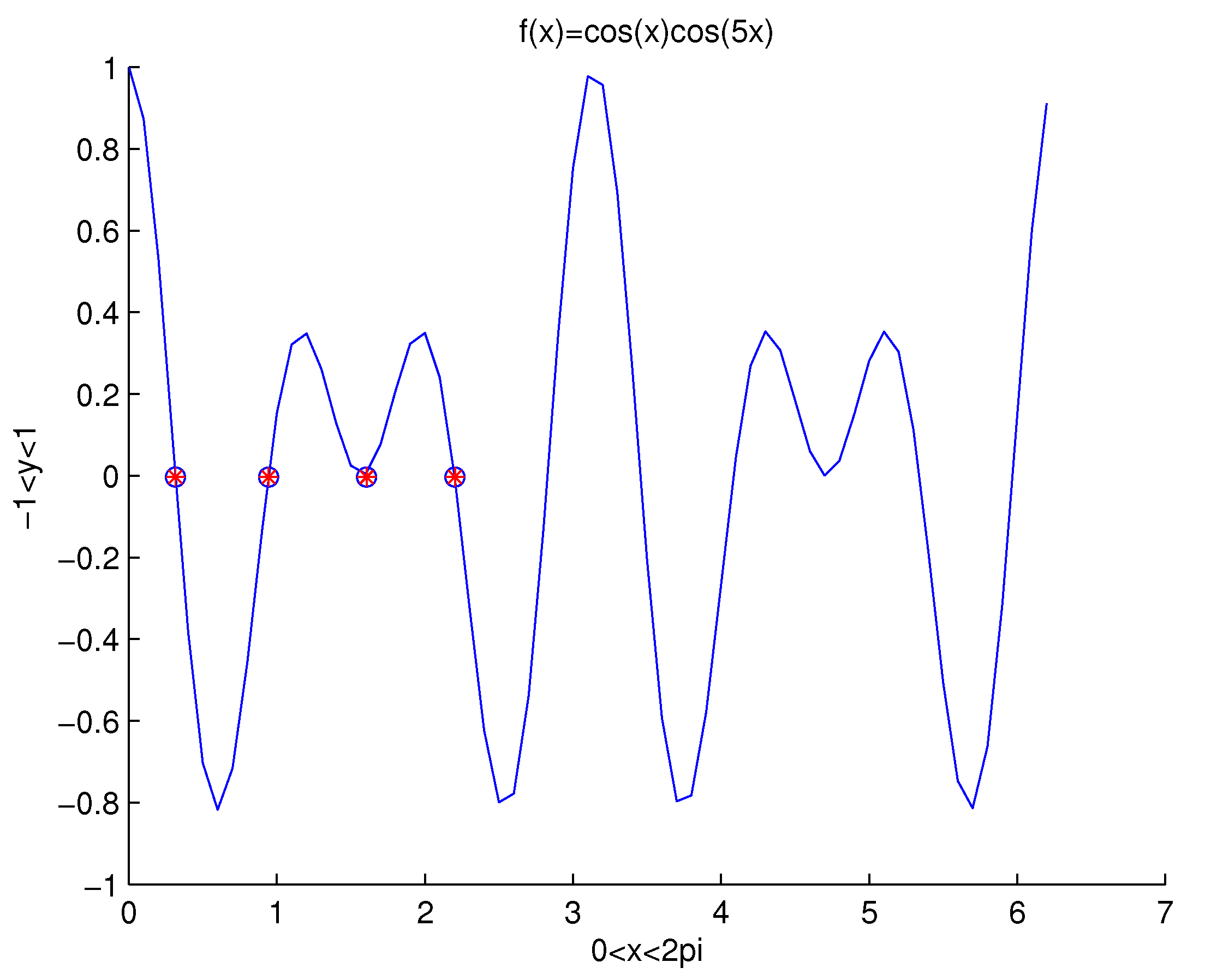
Theorem 9.

The sequence of eigenvalues of problem (4)–(8) has the following approximate formulas:

$$\sqrt{{\lambda }_{n,1}}=\frac{(2n-1)\pi }{2r}+O\left(\frac{1}{n}\right),$$

(39)

$$\sqrt{{\lambda }_{n,2}}=\frac{(2n-1)\pi }{2(a-r)}+O\left(\frac{1}{n}\right).$$

(40)

Proof. 

Because the problem’s eigenvalues are roots of $W1\left(\lambda \right)$ by Theorem 5, we have Equation (37), and then

$$\begin{array}{c}\hfill cos\left(s\left(r\right)\right)cos\left(s(r-a)\right)=O\left(\frac{1}{\left|s\right|}\right).\end{array}$$

(41)

Suppose that $f\left(s\right)$ and $g\left(s\right)$ are the left and right sides of Equation (41), respectively. It is easy to determine $\left|f\right(s\left)\right|\le \left|g\right(s\left)\right|$. Rouch’s theorem leads that $f\left(s\right)$ and $f\left(s\right)+g\left(s\right)$ have the same number of zeros. The roots of the function are similar to $\frac{(2n-1)\pi }{2r}$ or $\frac{(2n-1)\pi }{2(a-r)}$; see Figure 1. This is why we obtain (39) and (40). □

Figure 1. Approximate characteristic equation, where $r=1,a=6.$

This is from the approximate expressions of the linearly independent solutions, eigenvalues and the characteristic equation $W\left(\lambda \right)$. We shall create approximate formulas for eigenfunctions (see Reference [20], Theorem 4.1).

Theorem 10.

Approximate formulas for the eigenfunctions of (4)–(8) corresponding to the eigenvalues $\lambda n,1,lambdan,2$ include the following forms:

$$\begin{array}{c}\hfill {\varphi }_{n,1}(x,{\lambda }_{n,1})=cos\left(\frac{(2n-1)\pi }{2r}x\right)+O\left(\frac{1}{n}\right),\end{array}$$

(42)

$$\begin{array}{c}\hfill {\varphi }_{n,2}(x,{\lambda }_{n,2})=cos\left(\frac{(2n-1)\pi }{2(a-r)}(x-a)\right)+O\left(\frac{1}{n}\right).\end{array}$$

(43)

Proof. 

From calculations (22), (28)–(30), we can approximate ${\xi }_{11}(x,\lambda n,1)$, ${\xi }_{11}^{{}^{\prime }}(x,\lambda n,1)$, ${\varphi }_{21}(x,\lambda n,1)$, and ${\varphi }_{21}^{{}^{\prime }(x,\lambda n,1)}$ and replace them with an equation characteristic of $W\left(\lambda \right)$. A basic calculation (42) and (43) can therefore be obtained. □

Remember that, from (42), (43), we can check that the formulas (39) and (40) are simple. Generally speaking, the problem’s eigenvalues (4)–(8) are simple (see Reference [7], Theorem 4.2).

Example 1.

Consider the eigenvalue problem:

$$-y^{{}^{″}}(x,\lambda )+q\left(x\right)y(x,\lambda )=\lambda y(x,\lambda ),on[0,1)\cup (1,6],$$

(44)

with the following boundary:

$$y(0,\lambda )=0,y^{{}^{\prime }}(6,\lambda )+i\lambda y(6,\lambda )=0,$$

(45)

where

$$q\left(x\right)=\left\{\begin{array}{cc}1;\hfill & x\in [0,1)\hfill \\ 2;\hfill & x\in (1,6],\hfill \end{array}\right.$$

(46)

with the transmission conditions at $x=r$:

$$y(1+,\lambda )-y(1-,\lambda )+\lambda y^{{}^{\prime }}(1-,\lambda )=0,$$

(47)

$$y^{{}^{\prime }}(1+,\lambda )-y{}^{\prime }(1-,\lambda )+\lambda y(1-,\lambda )=0.$$

(48)

It is easy to see that, on the interval $[0,1)$, the eigenvalues of problem (45)–(48) are near to $\frac{(2n-1)\pi }{2}$, and, for sufficiently large n, and for each n, there is a corresponding eigenfunction of the form $cos\left(\frac{(2n-1)\pi }{2}x\right)$. In the same way, on the interval $(1,6]$, the eigenvalues of problem (45)–(48) are near $\frac{(2n-1)\pi }{10}$, and, for sufficiently large n, and for each n, there is a corresponding eigenfunction of the form $cos\left(\frac{(2n-1)\pi }{10}x\right)$ (see Figure 1).

5. Conclusions

In this article, we investigated the spectral properties of the Regge-type problem. First of all, we convert the problem for a linear operator in a special Krien space, and, according to this operator, we provide a formula for calculating the eigenvalues of the problem. Lastly, we obtained the simple and bounded eigenfunctions of the Regge-type problem (4)–(8).