On the Arcsecant Hyperbolic Normal Distribution. Properties, Quantile Regression Modeling and Applications

Abstract

This work proposes a new distribution defined on the unit interval. It is obtained by a novel transformation of a normal random variable involving the hyperbolic secant function and its inverse. The use of such a function in distribution theory has not received much attention in the literature, and may be of interest for theoretical and practical purposes. Basic statistical properties of the newly defined distribution are derived, including moments, skewness, kurtosis and order statistics. For the related model, the parametric estimation is examined through different methods. We assess the performance of the obtained estimates by two complementary simulation studies. Also, the quantile regression model based on the proposed distribution is introduced. Applications to three real datasets show that the proposed models are quite competitive in comparison to well-established models.

1. Introduction

Over the past twenty years, many statisticians and researchers have focused on proposing new extended or generalized distributions by adding additional parameters to the basic probability distributions. The common point of these studies is to obtain better inferences than those of the baseline probability distributions. In this context, especially, the modeling approaches on the unit interval have recently multiplied since they are related to specific issues such as the recovery rate, mortality rate, daily patient rate, etc. The beta distribution is the best-known distribution defined over the unit interval for modeling the above measures. It has great flexibility in the shapes of the probability density function (pdf) and hazard rate function (hrf). Although it has very flexible forms for data modeling, sometimes it is not sufficient for modeling and explaining unit datasets. For this reason, new alternative unit models have been proposed in the statistical distribution literature, including the Johnson $S_B$ [1], Topp-Leone [2], Kumaraswamy [3], standart two-sided power [4], log-Lindley [5], log-xgamma [6], unit Birnbaum-Saunders [7], unit Weibull [8], unit Lindley [9], unit inverse Gaussian [10], unit Gompertz [11], second degree unit Lindley [12], log-weighted exponential [13], logit slash [14], unit generalized half normal [15], unit Johnson $S_U$ [16], trapezoidal beta [17] and unit Rayleigh [18] distributions. Many of the above distributions were obtained by transforming the baseline distribution, and they performed better than the beta distribution in terms of data modeling. For instance, the Johnson $S_B$ distribution was created via logistic transformation of the ordinary normal distribution. In this way, a very flexible unit normal distribution was obtained over the unit interval. The other mentioned unit distributions introduced over the last decade can also be seen as alternatives to the well-known beta, Johnson $S_B$, Topp-Leone and Kumaraswamy distributions.

On the other hand, the ordinary regression models explain the response variable for given certain values of the covariates based on the conditional mean. However, the mean may be affected by a skewed distribution or outliers in the measurements. Possible solutions are provided by the quantile regression models proposed by [19], particularly popular for being less sensitive to outliers than the ordinary regression models.

In line with above, the aim of this study is to introduce a new alternative unit probability distribution based on the normal distribution. More precisely, we use a new transformation of the normal distribution based on the hyperbolic secant function. As a matter of fact, the use of the hyperbolic function has not received enough attention in the published literature on distribution theory, despite the great interest among students and practitioners of the few distributions based on it. Examples include the famous hyperbolic secant distribution and its generalizations as presented in [20]. In a sense, we show that the proposed methodology allows us to transport the applicability and working capacity of the normal distribution to the unit interval. In particular, we develop a new quantile regression modeling via the re-parameterizing of the new probability distribution in terms of any quantile. All these aspects are developed in the article through mathematical, graphical and numerical approaches.

The paper has been set as follows. We define the proposed distribution in Section 2. Its basic distributional properties are described in Section 3. Section 4 is devoted to the procedures of the different parametric estimation methods. Two different simulation studies are given to see the performance of the different estimates of the model parameters in Section 5. The new quantile regression model based on the proposed distribution and its residual analysis are introduced by Section 6. Three real data illustrations, one of which relates to quantile modeling and others to univariate data modeling, are illustrated in Section 7. Finally, the paper is ended with conclusions in Section 8.

2. The New Unit Distribution and Its Properties

The new unit distribution is defined as follows: Let Y be a random variable such that $Y\sim N(\mu ,{\sigma }^2)$ where $\mu \in \mathbb{R}$ and $\sigma >0$, and X be the random variable defined by

$$X=\mathrm{sech}Y,$$

where $\mathrm{sech}y=2/(e^y+e^{-y})=2e^y/(e^{2y}+1)\in (0,1)$ is the hyperbolic secant function for $y\in \mathbb{R}$, also known as the inverse of the hyperbolic cosine function. Then the distribution of X is called “arcsech” normal distribution and it is denoted by $ASHN$ or $ASHN(\mu ,\sigma )$ when $\mu$ and $\sigma$ are required. To our knowledge, it constitutes a new unit distribution; It is unlisted in the literature. Before stating the motivations for the $ASHN$ distribution, the corresponding cumulative distribution function (cdf) and pdf are presented in the following proposition.

Proposition 1.

The cdf and pdf of the $ASHN(\mu ,\sigma )$ distribution are given as

$$\begin{array}{c}\hfill F(x,\mu ,\sigma )=2-\mathsf{\Phi }\left(\frac{arcsechx+\mu }{\sigma }\right)-\mathsf{\Phi }\left(\frac{arcsechx-\mu }{\sigma }\right)\end{array}$$

(1)

and

$$\begin{array}{c}\hfill f(x,\mu ,\sigma )=\frac{1}{\sigma x\sqrt{1-x^2}}\left[\varphi \left(\frac{arcsechx+\mu }{\sigma }\right)+\varphi \left(\frac{arcsechx-\mu }{\sigma }\right)\right],\end{array}$$

(2)

respectively, for $x\in (0,1)$, where $arcsechz=log\left[\left(1+\sqrt{1-z^2}\right)/z\right]>0$ is the hyperbolic arcsecant function (or inverse hyperbolic secant function) for $z\in (0,1)$, $\mathsf{\Phi }\left(x\right)$ and $\varphi \left(x\right)$ are the cdf and pdf of the $N(0,1)$ distribution, respectively. For $x\notin (0,1)$, standard completions on these functions are performed.

For the sake of presentation, the proof of this result and those of the results to come are given in Appendix A.

Based on Proposition 1, as a first property, note that, for $\mu =0$ and $x\in (0,1)$, the cdf and pdf are reduced to the quite manageable functions:

$$\begin{array}{c}\hfill F(x,0,\sigma )=2\left[1-\mathsf{\Phi }\left(\frac{1}{\sigma }arcsechx\right)\right]\end{array}$$

(3)

and

$$\begin{array}{c}\hfill f(x,0,\sigma )=\frac{2}{\sigma x\sqrt{1-x^2}}\varphi \left(\frac{1}{\sigma }arcsechx\right).\end{array}$$

(4)

In full generality, for $x\in (0,1)$, an alternative formulation for the pdf is

$$f(x,\mu ,\sigma )=\sqrt{\frac{2}{\pi }}\frac{1}{\sigma x\sqrt{1-x^2}}{e}^{-\frac{{\left(arcsechx\right)}^2+{\mu }^2}{2{\sigma }^2}}cosh\left(\frac{\mu }{{\sigma }^2}arcsechx\right),$$

(5)

where $coshy=(e^y+e^{-y})/2$ is the hyperbolic cosine function for $y\in \mathbb{R}$. Eventually, we can express the cosh term in Equation (5) as

$$cosh\left(\frac{\mu }{{\sigma }^2}arcsechx\right)=\frac{1}{2}\left[{\left(\frac{1}{x}+\sqrt{\frac{1}{x^2}-1}\right)}^{\frac{\mu }{{\sigma }^2}}+{\left(\frac{1}{x}+\sqrt{\frac{1}{x^2}-1}\right)}^{-\frac{\mu }{{\sigma }^2}}\right].$$

Let us now focus on the behavior of $f(x,\mu ,\sigma )$ at the boundaries.

• When x tends to 0, since $arcsechx\sim -logx\to +\infty$ and it appears in power 2 the exponential term, we have $f(x,\mu ,\sigma )\to 0$.
• When x tends to 1, since $arcsech1=0$, we have

  $$f(x,\mu ,\sigma )\sim \frac{1}{\sqrt{\pi }}\frac{1}{\sigma \sqrt{1-x}}{e}^{-\frac{{\mu }^2}{2{\sigma }^2}}\to +\infty .$$
  If $\sigma$ is large and ${\mu }^2\approx 2{\sigma }^2$, or ${\mu }^2/2{\sigma }^2$ is large, the point $x=1$ appears as a “special singularity” in the following sense: The function $f(x,\mu ,\sigma )$ can decrease to 0 in the neighborhood of $x=1$, then suddenly explodes at $x=1$. This phenomenon is only punctual; this is not a particular disadvantage for statistical modeling purposes.

Also, from Equation (2), it can seen that

$$f(x,-\mu ,\sigma )=\frac{1}{\sigma x\sqrt{1-x^2}}\left[\varphi \left(\frac{arcsechx-\mu }{\sigma }\right)+\varphi \left(\frac{arcsechx+\mu }{\sigma }\right)\right]=f(x,\mu ,\sigma ).$$

This means that the pdf shapes of the $ASHN(\mu ,\sigma )$ distribution coincide with those of the $ASHN(-\mu ,\sigma )$ distribution. Another remark is that the $ASHN$ distribution can have one mode into $(0,1)$, and it corresponds to the x satisfying the following equation:

$$2{\sigma }^2{x}^2-{\sigma }^{2}arctanh\left(x\right)+\left(\sqrt{1-x^2}\right)arcsechx=0.$$

This equation is complex and needs a numerical treatment to determine the value of the mode, if it exists.

The hrf of the $ASHN(\mu ,\sigma )$ distribution is given by

$$\begin{array}{c}\hfill h(x,\mu ,\sigma )=\frac{\varphi \left(\frac{arcsechx+\mu }{\sigma }\right)+\varphi \left(\frac{arcsechx-\mu }{\sigma }\right)}{\sigma x\sqrt{1-x^2}\left[\mathsf{\Phi }\left(\frac{arcsechx+\mu }{\sigma }\right)+\mathsf{\Phi }\left(\frac{arcsechx-\mu }{\sigma }\right)-1\right]}.\end{array}$$

(6)

Some plots of $f(x,\mu ,\sigma )$ and $h(x,\mu ,\sigma )$ are shown in Figure 1.

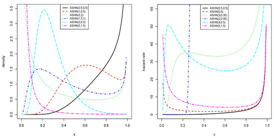
Figure 1. The possible pdf and hrf shapes of the $ASHN$ distribution.

From Figure 1, the flexibility of the obtained curves is flagrant; J, reversed J, U and bell shapes are observed for the pdf, whereas U, N and reversed J shapes are observed for the hrf. This panel of shapes is a plus for the $ASHN$ distribution, motivating its use for statistical modeling.

3. Distributional Properties

This section is devoted to some mathematical properties satisfied by the $ASHN$ distribution.

3.1. A Likelihood Ratio Order Result

The proposition below shows that the $ASHN$ distribution satisfies a strong intrinsic stochastic order result.

Proposition 2.

Let $X\sim ASHN(\mu ,{\sigma }_1)$ and $Y\sim ASHN(\mu ,{\sigma }_2)$ with $\mu =0$ and ${\sigma }_1>{\sigma }_2$. Then X is smaller than Y in likelihood ratio order.

In the general case where $\mu \ne 0$, there is no actual proof of such stochastic ordering properties. Further, let us mention that the likelihood order is a strong property, implying various stochastic orders such that the usual stochastic, hazard rate, reversed mean inactivity time, mean residual life and harmonic mean residual life orders, among others. We may refer the reader to [21] for all the theory and details about the concept of stochastic ordering.

3.2. Quantile Function

The theoretical definition of the quantile function (qf) of the $ASHN(\mu ,\sigma )$ distribution is the inverse function of Equation (1), that is

$$Q(y,\mu ,\sigma )=F^{-1}(y,\mu ,\sigma ),y\in (0,1).$$

In full generality, due to the complexity of $F(x,\mu ,\sigma )$, it is not possible to have a closed-form expression of this qf. However, in the case $\mu =0$, we arrive at

$$Q(y,\mu ,\sigma )=\mathrm{sech}\left[\sigma {\mathsf{\Phi }}^{-1}\left(1-\frac{y}{2}\right)\right],y\in (0,1),$$

where ${\mathsf{\Phi }}^{-1}\left(x\right)$ denotes the inverse function of $\mathsf{\Phi }\left(x\right)$, which also corresponds to the qf of the $N(0,1)$ distribution. In this case, the first quartile is obtained as $Q_1=Q(1/4,\mu ,\sigma )\approx \mathrm{sech}\left(\sigma \times 1.150349\right)$, the median is given by $M=Q(1/2,\mu ,\sigma )\approx \mathrm{sech}\left(\sigma \times 0.6744898\right)$, and the third quartile is defined by $Q_3=Q(3/4,\mu ,\sigma )\approx \mathrm{sech}\left(\sigma \times 0.3186394\right)$. Further, from $Q(y,\mu ,\sigma )$, one can generate values from the $ASHN$ distribution through basic simulation methods.

3.3. Moments

Let $X\sim ASHN(\mu ,\sigma )$. As prime definition, for any integer r, by denoting as E the expectation operator, the rth ordinary moment of X is defined by

$$\begin{array}{cc}\hfill m_r& =E\left(X^r\right)={\int }_0^1{x}^{r}f(x,\mu ,\sigma )dx\hfill \\ & =\frac{1}{\sigma }{\int }_0^1\frac{x^{r-1}}{\sqrt{1-x^2}}\left[\varphi \left(\frac{arcsechx+\mu }{\sigma }\right)+\varphi \left(\frac{arcsechx-\mu }{\sigma }\right)\right]dx.\hfill \end{array}$$

For the special case $\mu =0$, one can express it via the qf as

$$\begin{array}{c}\hfill m_r={\int }_0^1{\left[Q(y,\mu ,\sigma )\right]}^{r}dy={\int }_0^1{\left\{\mathrm{sech}\left[\sigma {\mathsf{\Phi }}^{-1}\left(1-\frac{y}{2}\right)\right]\right\}}^{r}dy.\end{array}$$

Clearly, there is no simple expression for $m_r$. When the parameters are fixed, it can be calculated numerically through standard numerical integration techniques. As the main analytical approach, one can consider a series expansion for $m_r$ as stated in the result below.

Proposition 3.

The rth moment of $X\sim ASHN(\mu ,\sigma )$ has the following expansion:

$$\begin{array}{cc}\hfill m_r& =2^r\left\{\sum _{k=0}^{+\infty }\left(\genfrac{}{}{0pt}{}{-r}{k}\right)e^{(2k+r)\mu }M\left(-\sigma (2k+r),\frac{\mu }{\sigma }\right)+\sum _{k=0}^{+\infty }\left(\genfrac{}{}{0pt}{}{-r}{k}\right)e^{-(2k+r)\mu }M\left(-\sigma (2k+r),-\frac{\mu }{\sigma }\right)\right\},\hfill \end{array}$$

where $M(x,a)=E\left[e^{xU}I(U>a)\right]$ with $U\sim N(0,1)$, $x\in \mathbb{R}$ and $a\in \mathbb{R}$, and $I(.)$ denotes the indicator function.

The function $M(x,a)$ introduced in Proposition 3 can be viewed as the upper incomplete version of the moment generating function of the $N(0,1)$ distribution. Naturally, it can be bounded from above as $M(x,a)\le E\left(e^{xU}\right)=e^{-\frac{x^2}{2}}$ for $x\in \mathbb{R}$ and $a\in \mathbb{R}$. By applying the Markov inequality, a lower is obtained as $M(x,a)\ge e^{xa}(1-\mathsf{\Phi }\left(a\right))$ for $x\ge 0$ and $a\in \mathbb{R}$.

Proposition 3 gives an analytical approach for mathematical manipulations or computations of $m_r$. Further, the following finite sum approximation is an immediate consequence:

$$\begin{array}{cc}\hfill m_r& \approx 2^r\left\{\sum _{k=0}^K\left(\genfrac{}{}{0pt}{}{-r}{k}\right)e^{(2k+r)\mu }M\left(-\sigma (2k+r),\frac{\mu }{\sigma }\right)+\sum _{k=0}^K\left(\genfrac{}{}{0pt}{}{-r}{k}\right)e^{-(2k+r)\mu }M\left(-\sigma (2k+r),-\frac{\mu }{\sigma }\right)\right\},\hfill \end{array}$$

where K denotes a reasonably large integer.

From the moments, we can derive other measures of interest for X. For instance, the mean of X is just $m_1$, the variance of X can be determined through the Koenig-Huyghens formula involving $m_1$ and $m_2$, that is $V=m_2-m_1^2$, the rth central moment defined by $m_r^c=E\left[{(X-m_1)}^r\right]$ can be expressed via $m_1,\dots ,m_r$ by using the binomial formula, the skewness coefficient of X is defined by $S=m_3^c{V}^{-\frac{3}{2}}$ and the kurtosis coefficient of X is given by $K=m_4^c{V}^{-2}$. These coefficients evaluate the “peakedness” and “tailedness” of the $ASHN$ distribution, respectively. Figure 2 represents these coefficients while varying the values for $\mu$ and $\sigma$.

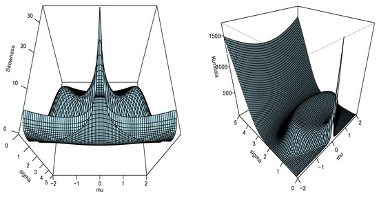
Figure 2. The skewness and kurtosis plots of the $ASHN$ distribution.

From Figure 2, we see that the skewness coefficient can be negative and positive, and the kurtosis coefficient can be either very small or very large. Both have a complex non-monotonic structure. These facts attest to the ability of the $ASHN$ distribution to adapt to various situations from heterogeneous unit data.

3.4. Order Statistics

The order statistics are important since they are involved in many statistical modeling and methods. Here, the basics of them in the context of the $ASHN$ distribution are described. Let $X_1,X_2,\dots ,X_n$ be a random sample from $X\sim ASHN(\mu ,\sigma )$, and $X_{\left(1\right)},X_{\left(2\right)},\dots ,X_{\left(n\right)}$ be the corresponding order statistics, that is $X_{\left(1\right)}\le X_{\left(2\right)}\le \dots \le X_{\left(n\right)}$. Then, the pdf of $X_{\left(i\right)}$ has the following general expression:

$$f_{X_{\left(i\right)}}(x,\mu ,\sigma )=\frac{n!}{(i-1)!(n-i)!}f(x,\mu ,\sigma ){\left[F(x,\mu ,\sigma )\right]}^{i-1}{[1-F(x,\mu ,\sigma )]}^{n-i}.$$

(7)

Owing to Equations (1) and (2), for $x\in (0,1)$, we obtain

$$\begin{array}{c}{f}_{X_{\left(i\right)}}(x,\mu ,\sigma )=\frac{n!}{(i-1)!(n-i)!}\frac{1}{\sigma x\sqrt{1-x^2}}\left[\varphi \left(\frac{arcsechx+\mu }{\sigma }\right)+\varphi \left(\frac{arcsechx-\mu }{\sigma }\right)\right]\times \hfill \\ {\left[2-\mathsf{\Phi }\left(\frac{arcsechx+\mu }{\sigma }\right)-\mathsf{\Phi }\left(\frac{arcsechx-\mu }{\sigma }\right)\right]}^{i-1}\times \hfill \\ {\left[\mathsf{\Phi }\left(\frac{arcsechx+\mu }{\sigma }\right)+\mathsf{\Phi }\left(\frac{arcsechx-\mu }{\sigma }\right)-1\right]}^{n-i}.\hfill \end{array}$$

The pdf of the extreme statistics $X_{\left(1\right)}$ and $X_{\left(n\right)}$ are derived by substituting $i=1$ and $i=n$ in the above equation, respectively. Other important results are that

$$\begin{array}{c}\hfill E\left[F(X_{\left(i\right)},\mu ,\sigma )\right]=\frac{i}{n+1},V\left[F(X_{\left(i\right)},\mu ,\sigma )\right]=\frac{i(n-i+1)}{(n+2){(n+1)}^2}.\end{array}$$

(8)

The order statistics, as well as their mean and variance, will be useful in the next section.

4. Different Methods of the Parameter Estimation

In this section, we point out some different estimators to estimate the parameters of the $ASHN$ model. More precisely, the maximum likelihood, maximum product spacings, least squares, weighted least squares, Anderson-Darling and Cramér-von Mises estimates are derived.

4.1. Maximum Likelihood Estimation

Let $X_1,X_2,\cdots ,X_n$ be a random sample from the $ASHN$ distribution with observed values $x_1,x_2,\cdots ,x_n,$ and $\mathsf{\Theta }={(\mu ,\sigma )}^T$ be the vector of the model parameters. Then, the log-likelihood function is given by

$$\begin{array}{cc}\hfill \ell =\ell \left(\mathsf{\Theta }\right)& =-nlog\sigma -\frac{n}{2}log\left(2\pi \right)-\sum _{i=1}^{n}log\left[x_i\sqrt{1-x_i^2}\right]-\frac{1}{2{\sigma }^2}\sum _{i=1}^n{\left(arcsech\left(x_i\right)-\mu \right)}^2\hfill \\ & +\sum _{i=1}^{n}log\left[1+e^{-\frac{2\mu }{{\sigma }^2}arcsech\left(x_i\right)}\right].\hfill \end{array}$$

(9)

Based on $\ell \left(\mathsf{\Theta }\right)$, the maximum likelihood estimations (MLEs) of $\mu$ and $\sigma$, say $\widehat{\mu }$ and $\widehat{\sigma }$, respectively, are obtained as

$$(\widehat{\mu },\widehat{\sigma })={\mathrm{argmax}}_{\mathsf{\Theta }\in \mathbb{R}\times (0,+\infty )}\ell \left(\mathsf{\Theta }\right).$$

Mathematically, this is equivalent to solve the following equations with respect to the parameters:

$$\frac{\partial \ell \left(\mathsf{\Theta }\right)}{\partial \mu }=\frac{1}{{\sigma }^2}\sum _{i=1}^n\left(arcsech\left(x_i\right)-\mu \right)-\frac{2}{{\sigma }^2}\sum _{i=1}^n\frac{arcsech\left(x_i\right)e^{-\frac{2\mu }{{\sigma }^2}arcsech\left(x_i\right)}}{1+e^{-\frac{2\mu }{{\sigma }^2}arcsech\left(x_i\right)}}=0$$

(10)

and

$$\frac{\partial \ell \left(\mathsf{\Theta }\right)}{\partial \sigma }=-\frac{n}{\sigma }+\frac{1}{{\sigma }^3}\sum _{i=1}^n{\left(arcsech\left(x_i\right)-\mu \right)}^2+\frac{4\mu }{{\sigma }^3}\sum _{i=1}^n\frac{arcsech\left(x_i\right)e^{-\frac{2\mu }{{\sigma }^2}arcsech\left(x_i\right)}}{1+e^{-\frac{2\mu }{{\sigma }^2}arcsech\left(x_i\right)}}=0.$$

(11)

From Equation (10), we have

$$\frac{1}{2}\sum _{i=1}^n\left(arcsech\left(x_i\right)-\mu \right)=\sum _{i=1}^n\frac{arcsech\left(x_i\right)e^{-\frac{2\mu }{{\sigma }^2}arcsech\left(x_i\right)}}{1+e^{-\frac{2\mu }{{\sigma }^2}arcsech\left(x_i\right)}}.$$

(12)

Substituting the right hand side of Equation (12) in Equation (11), the following equation is obtained for the desired solution for ${\sigma }^2$:

$$\begin{array}{c}\hfill {\sigma }^2=\frac{1}{n}\left[\sum _{i=1}^n{\left(arcsech\left(x_i\right)-\mu \right)}^2+2\mu \sum _{i=1}^n\left(arcsech\left(x_i\right)-\mu \right)\right]=\frac{1}{n}\sum _{i=1}^n{\left(arcsech\left(x_i\right)\right)}^2-{\mu }^2.\end{array}$$

(13)

Then, substituting Equation (13) in Equation (9), we obtain the profile log-likelihood according to $\mu$ as

$$\begin{array}{cc}\hfill \ell \left(\mu \right)=& -\frac{n}{2}log\left[\frac{1}{n}\sum _{i=1}^n{\left(arcsech\left(x_i\right)\right)}^2-{\mu }^2\right]-\frac{n}{2}log\left(2\pi \right)-\sum _{i=1}^{n}log\left[x_i\sqrt{1-x_i^2}\right]\hfill \\ & +\sum _{i=1}^{n}log\left[1+exp\left\{-2\mu arcsech\left(x_i\right){\left(\frac{1}{n}\sum _{i=1}^n{\left(arcsech\left(x_i\right)\right)}^2-{\mu }^2\right)}^{-1}\right\}\right]\hfill \\ & -\frac{{\displaystyle \sum _{i=1}^n}{\left(arcsech\left(x_i\right)-\mu \right)}^2}{2\left(\frac{1}{n}{\displaystyle \sum _{i=1}^n}{\left(arcsech\left(x_i\right)\right)}^2-{\mu }^2\right)}.\hfill \end{array}$$

Following the normal routine of the parameter estimation based on the profile log-likelihood function, we have

$$\begin{array}{c}\frac{\partial \ell \left(\mu \right)}{\partial \mu }=\frac{n\mu }{\frac{1}{n}{\displaystyle \sum _{i=1}^n}{\left(arcsech\left(x_i\right)\right)}^2-{\mu }^2}\hfill \\ -\frac{\mu {\displaystyle \sum _{i=1}^n}{\left(arcsech\left(x_i\right)-\mu \right)}^2-{\displaystyle \sum _{i=1}^n}\left(arcsech\left(x_i\right)-\mu \right)\left(\frac{1}{n}{\displaystyle \sum _{i=1}^n}{\left(arcsech\left(x_i\right)\right)}^2-{\mu }^2\right)}{{\left(\frac{1}{n}{\displaystyle \sum _{i=1}^n}{\left(arcsech\left(x_i\right)\right)}^2-{\mu }^2\right)}^2}\hfill \\ -{\displaystyle \sum _{i=1}^n}\frac{2arcsech\left(x_i\right)\left(\frac{1}{n}{\displaystyle \sum _{i=1}^n}{\left(arcsech\left(x_i\right)\right)}^2+4{\mu }^2\right)exp\left\{-2\mu arcsech\left(x_i\right){\left(\frac{1}{n}{\displaystyle \sum _{i=1}^n}{\left(arcsech\left(x_i\right)\right)}^2-{\mu }^2\right)}^{-1}\right\}}{{\left(\frac{1}{n}{\displaystyle \sum _{i=1}^n}{\left(arcsech\left(x_i\right)\right)}^2-{\mu }^2\right)}^2\left(1+exp\left\{-2\mu arcsech\left(x_i\right){\left(\frac{1}{n}{\displaystyle \sum _{i=1}^n}{\left(arcsech\left(x_i\right)\right)}^2-{\mu }^2\right)}^{-1}\right\}\right)}.\hfill \end{array}$$

Hence, the numerical methods are needed to obtain $\widehat{\mu }$. Once $\widehat{\mu }$ is obtained, the MLE $\widehat{\sigma }$ is obtained by taking the square root of ${\widehat{\sigma }}^2$ as governed by Equation (13).

The well-known theory of the maximum likelihood method states that, under mild regularity conditions, one can use the bivariate normal distribution with mean $\mu =(\mu ,\sigma )$ and covariance matrix $I^{-1}$, where

$$I=-{\left.\left(\begin{array}{cc}{\displaystyle \frac{{\partial }^2}{\partial {\mu }^2}\ell \left(\mathsf{\Theta }\right)}& {\displaystyle \frac{{\partial }^2}{\partial \mu \partial \sigma }\ell \left(\mathsf{\Theta }\right)}\\ {\displaystyle \frac{{\partial }^2}{\partial \mu \partial \sigma }\ell \left(\mathsf{\Theta }\right)}& {\displaystyle \frac{{\partial }^2}{\partial {\sigma }^2}\ell \left(\mathsf{\Theta }\right)}\end{array}\right)\right|}_{\mathsf{\Theta }=\widehat{\mathsf{\Theta }}},$$

to construct confidence intervals or likelihood ratio test on the parameters. The components of I can be derived through standard derivatives formula. Then, approximate $100(1-\vartheta )\%$ confidence intervals for $\mu$ and $\sigma$ can be determined by $\widehat{\mu }\pm z_{\vartheta /2}{s}_{\widehat{\mu }}$ and $\widehat{\sigma }\pm z_{\vartheta /2}{s}_{\widehat{\sigma }}$, respectively, where $z_{\vartheta /2}$ is the upper $(\vartheta /2)$th percentile of the standard normal distribution, $s_{\widehat{\mu }}$ is the first diagonal element of $I^{-1}$ and $s_{\widehat{\sigma }}$ is its second diagonal element. Thus defined, they are the (asymptotic) standard errors (SEs) of $\widehat{\mu }$ and $\widehat{\sigma }$, respectively.

4.2. Maximum Product Spacing Estimation

Cheng and Aming [22] have proposed the maximum product spacing (MPS) method as an alternative to the maximum likelihood method. It is based on the idea that differences (spacings) between the values of the cdf at consecutive data points should be identically distributed. Now, let $X_{\left(1\right)},X_{\left(2\right)},\dots ,X_{\left(n\right)}$ be the order statistics from the $ASHN$ distribution with sample size n, and $x_{\left(1\right)},x_{\left(2\right)},\dots ,x_{\left(n\right)}$ be the ordered observed values. Then, the MPS estimates (MPSEs) of $\mu$ and $\sigma$, say ${\widehat{\mu }}_{MPS}$ and ${\widehat{\sigma }}_{MPS}$, respectively, are given as

$$({\widehat{\mu }}_{MPS},{\widehat{\sigma }}_{MPS})={\mathrm{argmax}}_{\mathsf{\Theta }\in \mathbb{R}\times (0,+\infty )}MPS\left(\mathsf{\Theta }\right),$$

where

$$\begin{array}{c}\hfill MPS\left(\mathsf{\Theta }\right)=\frac{1}{n+1}\sum _{i=1}^{n+1}log\left[F(x_{\left(i\right)},\mu ,\sigma )-F(x_{(i-1)},\mu ,\sigma )\right].\end{array}$$

(14)

They are also given as the simultaneous solutions of the following equations:

$$\frac{\partial MPS\left(\mathsf{\Theta }\right)}{\partial \mu }=\frac{1}{n+1}\sum _{i=1}^{n+1}\left[\frac{F_{\mu }^{{}^{\prime }}(x_{\left(i\right)},\mu ,\sigma )-F_{\mu }^{{}^{\prime }}(x_{(i-1)},\mu ,\sigma )}{F(x_{\left(i\right)},\mu ,\sigma )-F(x_{(i-1)},\mu ,\sigma )}\right]=0$$

and

$$\frac{\partial MPS\left(\mathsf{\Theta }\right)}{\partial \sigma }=\frac{1}{n+1}\sum _{i=1}^{n+1}\left[\frac{F_{\sigma }^{{}^{\prime }}(x_{\left(i\right)},\mu ,\sigma )-F_{\sigma }^{{}^{\prime }}(x_{(i-1)},\mu ,\sigma )}{F(x_{\left(i\right)},\mu ,\sigma )-F(x_{(i-1)},\mu ,\sigma )}\right]=0,$$

where

$$F_{\mu }^{{}^{\prime }}(x,\mu ,\sigma )=\frac{1}{\sigma }\left[\varphi \left(\frac{arcsechx-\mu }{\sigma }\right)-\varphi \left(\frac{arcsechx+\mu }{\sigma }\right)\right]$$

and

$$F_{\sigma }^{{}^{\prime }}(x,\mu ,\sigma )=\frac{1}{{\sigma }^2}\left[\left(arcsechx-\mu \right)\varphi \left(\frac{arcsechx-\mu }{\sigma }\right)+\left(arcsechx+\mu \right)\varphi \left(\frac{arcsechx+\mu }{\sigma }\right)\right].$$

4.3. Least Squares Estimation

The least square estimates (LSEs) of $\mu$ and $\sigma$, say ${\widehat{\mu }}_{LSE}$ and ${\widehat{\sigma }}_{LSE}$, respectively, are obtained as

$$({\widehat{\mu }}_{LSE},{\widehat{\sigma }}_{LSE})={\mathrm{argmin}}_{\mathsf{\Theta }\in \mathbb{R}\times (0,+\infty )}LSE\left(\mathsf{\Theta }\right),$$

where

$$LSE\left(\mathsf{\Theta }\right)=\sum _{i=1}^n{\left(F(x_{\left(i\right)},\mu ,\sigma )-E\left[F(X_{\left(i\right)},\mu ,\sigma )\right]\right)}^2,$$

(15)

where, by Equation (8), $E\left[F(X_{\left(i\right)},\mu ,\sigma )\right]=i/(n+1)$ for $i=1,2,\dots ,n$. Then, ${\widehat{\mu }}_{LSE}$ and ${\widehat{\sigma }}_{LSE}$ are solutions of the following equations:

$$\frac{\partial LSE\left(\mathsf{\Theta }\right)}{\partial \mu }=2\sum _{i=1}^n{F}_{\mu }^{{}^{\prime }}(x_{\left(i\right)},\mu ,\sigma )\left(F(x_{\left(i\right)},\mu ,\sigma )-\frac{i}{n+1}\right)=0$$

and

$$\frac{\partial LSE\left(\mathsf{\Theta }\right)}{\partial \sigma }=2\sum _{i=1}^n{F}_{\sigma }^{{}^{\prime }}(x_{\left(i\right)},\mu ,\sigma )\left(F(x_{\left(i\right)},\mu ,\sigma )-\frac{i}{n+1}\right)=0,$$

where $F_{\mu }^{{}^{\prime }}(x_{\left(i\right)},\mu ,\sigma )$ and $F_{\sigma }^{{}^{\prime }}(x_{\left(i\right)},\mu ,\sigma )$ are mentioned before.

4.4. Weighted Least Squares Estimation

Similarly to LSEs, the weighted least square estimates (WLSEs) of $\mu$ and $\sigma$, say ${\widehat{\mu }}_{WLSE}$ and ${\widehat{\sigma }}_{WLSE}$, respectively, are given as

$$({\widehat{\mu }}_{WLSE},{\widehat{\sigma }}_{WLSE})={\mathrm{argmin}}_{\mathsf{\Theta }\in \mathbb{R}\times (0,+\infty )}WLSE\left(\mathsf{\Theta }\right),$$

where

$$WLSE\left(\mathsf{\Theta }\right)=\sum _{i=1}^n\frac{1}{V\left[F(X_{\left(i\right)},\mu ,\sigma )\right]}{\left(F(x_{\left(i\right)},\mu ,\sigma )-E\left[F(X_{\left(i\right)},\mu ,\sigma )\right]\right)}^2,$$

(16)

where, by Equation (8), $E\left[F(X_{\left(i\right)},\mu ,\sigma )\right]=i/(n+1)$ and $V\left[F(X_{\left(i\right)},\mu ,\sigma )\right]=i(n-i+1)/\left[(n+2){(n+1)}^2\right]$ for $i=1,2,\dots ,n$. Then, ${\widehat{\mu }}_{WLSE}$ and ${\widehat{\sigma }}_{WLSE}$ are solutions of the following equations:

$$\frac{\partial WLSE\left(\mathsf{\Theta }\right)}{\partial \mu }=2\sum _{i=1}^n\frac{(n+2){(n+1)}^2}{i(n-i+1)}\left(F(x_{\left(i\right)},\mu ,\sigma )-\frac{i}{n+1}\right)F_{\mu }^{{}^{\prime }}(x_{\left(i\right)},\mu ,\sigma )=0$$

and

$$\frac{\partial WLSE\left(\mathsf{\Theta }\right)}{\partial \sigma }=2\sum _{i=1}^n\frac{(n+2){(n+1)}^2}{i(n-i+1)}\left(F(x_{\left(i\right)},\mu ,\sigma )-\frac{i}{n+1}\right)F_{\sigma }^{{}^{\prime }}(x_{\left(i\right)},\mu ,\sigma )=0.$$

4.5. Anderson-Darling Estimation

The Anderson-Darling minimum distance estimates (ADEs) of $\mu$ and $\sigma$, say ${\widehat{\mu }}_{AD}$ and ${\widehat{\sigma }}_{AD}$, respectively, are determined as

$$({\widehat{\mu }}_{AD},{\widehat{\sigma }}_{AD})={\mathrm{argmin}}_{\mathsf{\Theta }\in \mathbb{R}\times (0,+\infty )}AD\left(\mathsf{\Theta }\right),$$

where

$$AD\left(\mathsf{\Theta }\right)=-n-\sum _{i=1}^n\frac{2i-1}{n}\left\{log\left[F(x_{\left(i\right)},\mu ,\sigma )\right]+log\left[1-F(x_{(n+1-i)},\mu ,\sigma )\right]\right\}.$$

(17)

Therefore, ${\widehat{\mu }}_{AD}$ and ${\widehat{\sigma }}_{AD}$ can be obtained as the solutions of the following system of equations:

$$\frac{\partial AD\left(\mathsf{\Theta }\right)}{\partial \mu }=-\sum _{i=1}^n\frac{2i-1}{n}\left[\frac{F_{\mu }^{\prime }(x_{\left(i\right)},\mu ,\sigma )}{F(x_{\left(i\right)},\mu ,\sigma )}-\frac{F_{\mu }^{\prime }(x_{\left(n+1-i\right)},\mu ,\sigma )}{1-F(x_{(n+1-i)},\mu ,\sigma )}\right]=0$$

and

$$\frac{\partial AD\left(\mathsf{\Theta }\right)}{\partial \sigma }=-\sum _{i=1}^n\frac{2i-1}{n}\left[\frac{F_{\sigma }^{\prime }\left(x_{\left(i\right)},\mu ,\sigma \right)}{F(x_{\left(i\right)},\mu ,\sigma )}-\frac{F_{\sigma }^{\prime }(x_{\left(n+1-i\right)},\mu ,\sigma )}{1-F(x_{(n+1-i)},\mu ,\sigma )}\right]=0.$$

4.6. The Cramér-von Mises Estimation

The Cramér-von Mises minimum distance estimates (CVMEs) of $\mu$ and $\sigma$, say ${\widehat{\mu }}_{CVM}$ and ${\widehat{\sigma }}_{CVM}$, respectively, are specified as

$$({\widehat{\mu }}_{CVM},{\widehat{\sigma }}_{CVM})={\mathrm{argmin}}_{\mathsf{\Theta }\in \mathbb{R}\times (0,+\infty )}CVM\left(\mathsf{\Theta }\right),$$

where

$$CVM\left(\mathsf{\Theta }\right)=\frac{1}{12n}+\sum _{i=1}^n{\left[F(x_{\left(i\right)},\mu ,\sigma )-\frac{2i-1}{2n}\right]}^2.$$

(18)

Therefore, the estimates ${\widehat{\mu }}_{CVM}$ and ${\widehat{\sigma }}_{CVM}$ can be obtained as the solutions of the following system of equations:

$$\frac{\partial CVM\left(\mathsf{\Theta }\right)}{\partial \mu }=2\sum _{i=1}^n\left(F(x_{\left(i\right)},\mu ,\sigma )-\frac{2i-1}{2n}\right)F_{\mu }^{\prime }(x_{\left(i\right)},\mu ,\sigma )=0$$

and

$$\frac{\partial CVM\left(\mathsf{\Theta }\right)}{\partial \sigma }=2\sum _{i=1}^n\left(F(x_{\left(i\right)},\mu ,\sigma )-\frac{2i-1}{2n}\right)F_{\sigma }^{\prime }(x_{\left(i\right)},\mu ,\sigma )=0.$$

All the presented equations contain complex non-linear functions; it is not possible to obtain explicit forms of all estimates. Therefore, they need to be solved through numerical methods such as the Newton-Raphson and quasi-Newton algorithms. In addition, Equations (9) and (14)–(18) can be also optimized directly by using the software such as R (constrOptim and optim), S-Plus and Matlab to numerically optimize $\ell \left(\mathsf{\Theta }\right)$, $MPS\left(\mathsf{\Theta }\right)$, $LSE\left(\mathsf{\Theta }\right)$, $WLSE\left(\mathsf{\Theta }\right)$, $AD\left(\mathsf{\Theta }\right)$ and $CVM\left(\mathsf{\Theta }\right)$ functions.

5. Empirical Simulations

In this section, we perform two graphical simulation studies to see the performance of the above estimates with varying sample size n. We generate $N=1000$ samples of size $n=20,25,\dots ,1000$ from the $ASHN$ distribution based on the following parameter values: ($\mu =2$, $\sigma =2$) and ($\mu =0.5$, $\sigma =0.5$) for the first and second simulation studies, respectively. The random numbers generation is obtained by the qf of the model. All the estimates based on the estimation methods are obtained by using the constrOptim function in the R program. Further, we calculate the empirical mean, bias and mean square error (MSE) of the estimates for comparisons between the methods. For $ϵ=\mu$ or $ϵ=\sigma$, the bias and MSE associated to $ϵ$ are calculated by

$$\begin{array}{c}\hfill Bia{s}_{ϵ}\left(n\right)=\frac{1}{N}\sum _{i=1}^N(ϵ-{\widehat{ϵ}}_i),MS{E}_{ϵ}\left(n\right)=\frac{1}{N}\sum _{i=1}^N{(ϵ-{\widehat{ϵ}}_i)}^2,\end{array}$$

respectively, where i is related to the ith sample. We expect that the empirical means are close to true values when the MSEs and biases are near zero. The results of this simulation study are shown in Figure 3 and Figure 4.

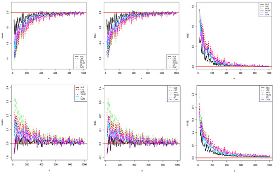
Figure 3. The results related to $\mu$ (top) and $\sigma$ (bottom) for the first simulation study.

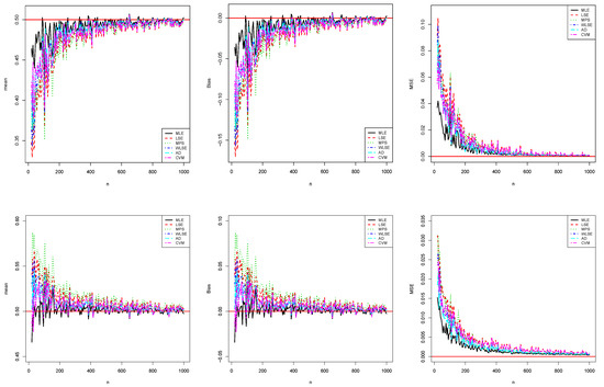
Figure 4. The results related to $\mu$ (top) and $\sigma$ (bottom) for the second simulation study.

Figure 3 and Figure 4 show that all estimates are consistent since the MSE and biasedness decrease to zero with increasing sample size as expected. One can state that all estimates are asymptotic unbiased. According to these two simulation studies, the amount of the biases and MSEs of the MLE method are smaller than those of the other methods for both parameters. Therefore, the ;MLE method can be chosen as more reliable than other methods of the newly defined model. Generally, the performances of all estimates are close when sample size increases. The similar results can be seen for different parameter values.

Moreover, we also give simulation study of the MLEs based on their 95% confidence intervals. In this regard, we use the coverage probability (CP) criteria defined by

$$C{P}_{ϵ}\left(n\right)=\frac{1}{N}\sum _{i=1}^{N}I(\widehat{{ϵ}_i}\pm 1.95996s_{\widehat{{ϵ}_i}}),$$

where $s_{{\widehat{ϵ}}_i}$ is the SE of the MLE ${\widehat{ϵ}}_i$. Figure 5 displays the obtained simulation results. From Figure 5, as expected, for each parameter, the CPs converge to the nominal value, that is 0.95, when sample size increases. The simulation results verify the consistency property of the MLEs.

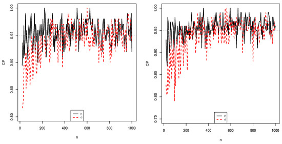
Figure 5. Estimated CPs for the first (left) and second (right) simulation studies.

6. A New Quantile Regression Model Based on the Special $\mathit{ASHN}$ Distribution

6.1. Motivation

The quantile regression has been developed in the seminal work of [19] as a way to model the conditional quantiles of an outcome variable as a function of covariates (regressors). Since this analysis aims to model the conditional quantiles of the response variable, it is a good robust alternative model to the ordinary LSE model, which estimates the conditional mean of the response variable. This is because the mean is affected by a skewed distribution or outliers in the measurements. Hence, the quantile response regression model will be less sensitive to outliers than the mean response regression model.

On the other hand, if the support of the response variable is defined on the unit interval, one can use an unit regression model based on an unit distribution for modeling the conditional mean or quantiles of the response variable via covariates. The beta regression [23] model first comes to mind to relate to continuous unit mean response variables in the unit interval with covariates. One may also see [12,13,24,25,26] for alternative unit mean response regression models to beta regression models. If the conditional dependent variable is skewed or has outliers, the quantile response modeling may be more appropriate when compared with the mean response modeling. The model is also motivated by the natural idea of replacing mean by median as a central tendency measure when the response data is severely asymmetric [27].

On the other hand, with the re-parameterizing the probability distribution as a function of the quantile approach, the Kumaraswamy [28,29] and unit Weibull [30] quantile regression models have been proposed for modeling the conditional quantiles of the unit response. One may also refer to [27,31,32,33,34] for alternative quantile response regression models. On the basis of these references, we want to propose an alternative quantile regression model considering a parameterization of the $ASHN$ distribution in terms of its any quantile. More precisely, the re-parameterizing process is applied via a scale parameter as being a quantile of the of the $ASHN$ distribution.

6.2. Proposed Quantile Regression Model

Now, we can focus on introducing an alternative quantile regression model based on a special $ASHN(\mu ,\sigma )$ distribution. Since the $ASHN$ distribution has not an explicit qf, we propose another distribution based on a special $ASHN$ distribution. We call it exponentiated $ASHN$ ($EASHN$) distribution. Its cdf and pdf are given by

$$\begin{array}{c}\hfill G(y,\alpha ,\sigma )={\left[2-2\mathsf{\Phi }\left(\frac{1}{\sigma }arcsechy\right)\right]}^{\alpha }\end{array}$$

(19)

and

$$\begin{array}{c}\hfill g(y,\alpha ,\sigma )=\frac{2\alpha }{\sigma y\sqrt{1-y^2}}\varphi \left(\frac{1}{\sigma }arcsechy\right){\left[2-2\mathsf{\Phi }\left(\frac{1}{\sigma }arcsechy\right)\right]}^{\alpha -1},\end{array}$$

respectively, where $y\in (0,1)$ and $\alpha ,\sigma >0$. For $y\notin (0,1)$, standard completions on these functions are performed. The cdf in Equation (19) is obtained as the exponentiated $ASHN(0,\sigma )$ distribution, that is $G(y,\alpha ,\sigma )={\left[F(y,0,\sigma )\right]}^{\alpha }$. We can call this model as Lehmann type I $ASHN$ model.

The qf of the $EASHN$ distribution is given by

$$Q(u,\alpha ,\sigma )=\mathrm{sech}\left[\sigma {\mathsf{\Phi }}^{-1}\left(1-\frac{u^{\frac{1}{\alpha }}}{2}\right)\right],$$

where $u\in (0,1)$. We are also motivated with the quantile regression modeling thanks to its manageable qf. Then, the pdf of the $EASHN$ distribution can be re-parameterized in terms of its uth quantile as $\eta =Q(u,\alpha ,\sigma )$. Let $\sigma =arcsech\eta /{\mathsf{\Phi }}^{-1}\left[(2-u^{1/\alpha })/2\right]$. Then, the cdf and pdf of the re-parameterized distribution are given by

$$\begin{array}{c}\hfill G(y,\alpha ,\eta )={\left[2-2\mathsf{\Phi }\left(\frac{{\mathsf{\Phi }}^{-1}\left(1-u^{\frac{1}{\alpha }}/2\right)}{arcsech\eta }arcsechy\right)\right]}^{\alpha }\end{array}$$

(20)

and

$$\begin{array}{c}g(y,\alpha ,\eta )=\frac{2\alpha {\mathsf{\Phi }}^{-1}\left(1-u^{\frac{1}{\alpha }}/2\right)}{arcsech\eta y\sqrt{1-y^2}}\varphi \left(\frac{{\mathsf{\Phi }}^{-1}\left(1-u^{\frac{1}{\alpha }}/2\right)}{arcsech\eta }arcsechy\right)\hfill \\ \times {\left[2-2\mathsf{\Phi }\left(\frac{{\mathsf{\Phi }}^{-1}\left(1-u^{\frac{1}{\alpha }}/2\right)}{arcsech\eta }arcsechy\right)\right]}^{\alpha -1},\hfill \end{array}$$

(21)

respectively, where $\alpha >0$ is the shape parameter. The parameter $\eta \in (0,1)$ represents the quantile parameter and it is assumed that u is known. A random variable Y having the pdf in Equation (21) is denoted by $Y\sim EASHN(\alpha ,\eta ,u)$. Some possible shapes of the re-parameterized model are shown in Figure 6. We see that the possible pdf shapes of the $EASHN$ distribution are the skewed shapes as well as U-shapes, N-shapes and increasing shapes.

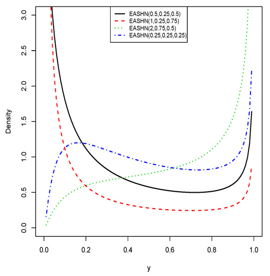
Figure 6. The pdf shapes of the re-parameterized $EASHN$ distribution.

We present the quantile regression model based on the $EASHN$ distribution with pdf in Equation (21). Let $y_1,y_2,\dots ,y_n$ be n random observations from the re-parameterized distribution such that, for $i=1,\dots ,n$, $y_i$ is a realization of $Y\sim EASHN(\alpha ,{\eta }_i,u)$, with unknown parameters ${\eta }_i$ and $\beta$, recalling that the parameter u is known. Then the $EASHN$ quantile regression model is defined as

$$g\left({\eta }_i\right)={\mathbf{x}}_i{\mathit{\beta }}^T,$$

where $\mathit{\beta }={\left({\beta }_0,{\beta }_1,{\beta }_2,\dots ,{\beta }_p\right)}^T$ and ${\mathbf{x}}_i=\left(1,x_{i1},x_{i2},x_{i3},\dots ,x_{ip}\right)$ are the unknown regression parameter vector and known ith vector of the covariates. Thus defined, $g\left(x\right)$ is the link function which is used to link the covariates to conditional quantile of the response variable. For instance, when $u=0.5$, the covariates are linked to conditional median of the response variable. The choice of the appropriate link function should be done considering the domain of the distribution.

6.3. Parameter Estimation

The unknown parameters of the $EASHN$ quantile regression model are obtained by means of the MLE method. Since the $EASHN$ distribution is defined on the unit interval, we use the logit-link function, that is

$$g\left({\eta }_i\right)=\mathrm{logit}\left({\eta }_i\right)=log\left(\frac{{\eta }_i}{1-{\eta }_i}\right)={\mathbf{x}}_i{\mathit{\beta }}^T,$$

implying that

$${\eta }_i=\frac{exp\left({\mathbf{x}}_i{\mathit{\beta }}^T\right)}{1+exp\left({\mathbf{x}}_i{\mathit{\beta }}^T\right)}.$$

(22)

By putting Equation (22) into Equation (21), the log-likelihood function of the $EASHN$ quantile regression model is

$$\begin{array}{c}\ell \left(\mathbf{\Omega }\right)=nlog2-\frac{n}{2}log\left(2\pi \right)+nlog\alpha +nlog\left[{\mathsf{\Phi }}^{-1}\left(1-\frac{u^{\frac{1}{\alpha }}}{2}\right)\right]\hfill \\ -\sum _{i=1}^{n}log\left[arcsech\left({\eta }_i\right)\left(y_i\sqrt{1-y_i^2}\right)\right]-\frac{1}{2}{\left[{\mathsf{\Phi }}^{-1}\left(1-\frac{u^{\frac{1}{\alpha }}}{2}\right)\right]}^2\sum _{i=1}^n{\left(\frac{arcsech\left(y_i\right)}{arcsech\left({\eta }_i\right)}\right)}^2\hfill \\ +(\alpha -1)\sum _{i=1}^{n}log\left[2-2\mathsf{\Phi }\left(\frac{arcsech\left(y_i\right)}{arcsech\left({\eta }_i\right)}{\mathsf{\Phi }}^{-1}\left(1-\frac{u^{\frac{1}{\alpha }}}{2}\right)\right)\right],\hfill \end{array}$$

(23)

where $\mathbf{\Omega }=\left(\alpha ,\mathit{\beta }\right)$ denotes the unknown parameter vector. Since Equation (23) includes nonlinear function according to model parameters, it can be maximized directly by software such as R, S-Plus, and Mathematica. Note that, when $u=0.5$, this is equivalent to modeling the conditional median. Under mild conditions of regularity, the asymptotic distribution of $\left(\widehat{\mathbf{\Omega }}-\mathbf{\Omega }\right)$ is multivariate normal $N_{p+1}\left(0,J^{-1}\right)$, where variance-covariance matrix $J^{-1}$ is defined by the inverse of the expected information matrix. For practical aims, we can use the observed information matrix instead of J. The elements of this observed information matrix are evaluated numerically by the software. We use the maxLik function implemented in the R software to maximize Equation (23) (see [35]). This function also gives asymptotic SEs numerically, which are obtained by the observed information matrix.

6.4. Residual Analysis

Residual analysis may be necessary to verify if the regression model is suitable. To see this, we work with the randomized quantile residuals [36] and the Cox-Snell residuals [37].

For $i=1,\dots ,n$, the ith randomized quantile residual is defined by

$${\widehat{r}}_i={\mathsf{\Phi }}^{-1}\left[G(y_i,\widehat{\alpha },{\widehat{\eta }}_i)\right],$$

where $G(y,\alpha ,\eta )$ is the cdf of the re-parameterized $EASHN$ distribution specified by Equation (20) and ${\widehat{\eta }}_i$ is defined by Equation (22) with $\widehat{\mathit{\beta }}$ replacing $\mathit{\beta }$. If the fitted model successfully processes the dataset, the distribution of the randomized quantile residuals will distribute the standard normal distribution.

Alternatively, for $i=1,\dots ,n$, the ith Cox and Snell residual is given by

$${\widehat{e}}_i=-log\left[1-G(y_i,\widehat{\alpha },{\widehat{\eta }}_i)\right].$$

If the model fits to data accordingly, the distribution of the Cox and Snell residuals will distribute a standard exponential distribution, that is with scale parameter 1.

7. Data Analysis

To emphasize the importance of the modeling ability of the $ASHN$ normal distribution, this section is devoted to three real data applications for both univariate data and quantile modelings.

7.1. Univariate Real Data Modeling

Here, we provide applications to two real datasets to prove empirically the potentiality of the $ASHN$ model. The proposed model is compared with some well-known two-parameter unit distributions in the literature, namely:

• Beta distribution.
  The two-parameter beta pdf is given by

  $$f_{Beta}(x,\mu ,\sigma )=\frac{1}{\mathrm{B}\left(\mu ,\sigma \right)}{x}^{\mu -1}{\left(1-x\right)}^{\sigma -1},x\in (0,1),$$

  where $\mu >0$ and $\sigma >0$ are shape parameters, and $\mathrm{B}(\mu ,\sigma )$ is the classical beta function.
• Kumaraswamy (Kw) distribution (see [3]).
  The two-parameter Kw pdf is expressed as

  $$f_{Kw}(x,\mu ,\sigma )=\mu \sigma x^{\mu -1}{\left(1-x^{\mu }\right)}^{\sigma -1},x\in (0,1),$$

  where $\mu >0$ and $\sigma >0$ are shape parameters.
• Johnson $S_B$ distribution (see [1]).
  The two-parameter Johnson $S_B$ pdf is given by

  $$f_{S_B}(x,\mu ,\sigma )=\frac{\sigma }{x\left(1-x\right)}\varphi \left[\sigma log\left(\frac{x}{1-x}\right)+\mu \right],x\in (0,1),$$

  where $\mu \in \mathbb{R}$ and $\sigma >0$ are shape parameters, and $\varphi (·)$ is the pdf of the standard normal distribution. For each model, we estimate the unknown parameters using the maximum likelihood approach.

Two datasets are considered. For them, in order to determine the optimum model, we compute the estimated log-likelihood values $\widehat{\ell }$, Akaike Information Criteria (AIC), Bayesian Information Criteria (BIC), Kolmogorov-Smirnov (KS), Anderson-Darling ($A^{*}$) and Cramér-von Mises ($W^{*}$) goodness-of-fit statistics for all models. In general, it can be chosen as the best model the one with the smaller values of the AIC, BIC, KS, $A^{*}$ and $W^{*}$ statistics and the larger values of $\widehat{\ell }$. The p-value of the KS test is also considered; more it is close to 1, better is the model. All computations are performed by using the maxLik [35] and goftest routines in the R software.

7.1.1. Data Analysis I

First, we consider an application to real dataset to show the modeling ability of the proposed distribution. The dataset introduces failure times of the 20 mechanical components given in [38]. The data are: 0.067, 0.068, 0.076, 0.081, 0.084, 0.085, 0.085, 0.086, 0.089, 0.098, 0.098, 0.114, 0.114, 0.115, 0.121, 0.125, 0.131, 0.149, 0.160, 0.485. Recently, these data was analyzed via different approaches by [15,39,40].

Table 1 lists the MLEs of the parameters and their SEs from the above fitted models and the values of the statistics: $\widehat{\ell }$, AIC, BIC, $A^{*}$, $W^{*}$ and KS goodness-of-fit statistics. As it can be seen, the results indicate that the $ASHN$ model has the smallest values of these statistics among the fitted models, and therefore it could be considered as the best model. The p-value of the KS test confirms this claim.

Table 1. MLEs, SEs of the estimates (in parentheses), $\widehat{\ell }$ and goodness-of-fits statistics for the first dataset (p-value is given in $[·]$).

Model	$\widehat{\mathit{\mu }}$	$\widehat{\mathit{\sigma }}$	$\widehat{\mathit{\ell }}$	$\mathit{AIC}$	$\mathit{BIC}$	${\mathit{A}}^{*}$	${\mathit{W}}^{*}$	$\mathit{KS}$
ASHN	2.9179	0.4322	33.2443	−62.4885	−60.4970	1.1850	0.1664	0.1746
	(0.0966)	(0.0684)						[0.5754]
Beta	3.1126	21.8245	27.8813	−51.7626	−49.7711	2.2611	0.3726	0.2537
	(1.0287)	(7.7997)						[0.1521]
Kw	1.5877	21.8673	25.6484	−47.2968	−45.3054	2.6889	0.4681	0.2626
	(0.3966)	17.9755						[0.1265]
Johnson $S_B$	3.8952	1.8605	31.3599	−58.7198	−56.7283	1.5531	0.2307	0.2039
	(0.6554)	(0.2942)						[0.3765]

The plots of the fitted pdfs and cdfs are displayed in Figure 7. These plots show that the $ASHN$ model provides the correct fit to these data compared to other models. Further, it captures data skewness and kurtosis better than other models.

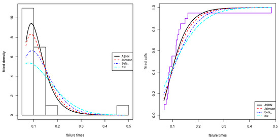
Figure 7. The fitted plots for the first dataset.

Figure 8 shows plots of the profile log-likelihood (PLL) functions for the parameters $\mu$ and $\sigma$ based on the first dataset. We observe that the likelihood equations have unique solutions for the MLEs.

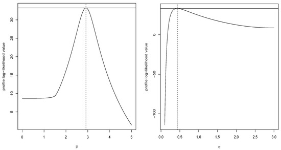
Figure 8. The plots of the PLL functions for the first dataset.

7.1.2. Data Analysis II

Here, the Better Life Index (BLI) dataset is used to illustrate the usefulness of the $ASHN$ distribution. The dataset can be found via link https://stats.oecd.org/index.aspx?DataSetCode=BLI2015. The BLI dataset is used to classify the OECD (Organisation for Economic Co-operation and Development) countries with 11 indicators and 24 variables as well as non-OECD economies such as Brazil and Russia. Here, we use an indicator that is entitled Job security as the dataset. This indicator presents the probability to become unemployed. Recently, these data was analyzed by [14]. We give the summary statistics of the dataset in Table 2. The data are right-skewed and have a consequent kurtosis.

Table 2. Some summary statistics of the second dataset.

Minimum	Mean	Median	Maximum	Variance	Skewness	Kurtosis	n
0.0240	0.0567	0.0515	0.1780	0.0007	2.7117	12.0173	36

Table 3 lists the MLEs, their SEs, $\widehat{\ell }$ and goodness-of-fits statistics from the fitted models for this dataset. Table 3 shows that the proposed model could be chosen as the best model among the fitted models since it has the lowest values of the AIC, BIC, $A^{*}$, $W^{*}$ and KS statistics and have the biggest $\widehat{\ell }$ value. It also has the biggest p-value of the KS test.

Table 3. MLEs, SEs of the estimates (in parentheses), $\widehat{\ell }$ and goodness-of-fits statistics for the second dataset (p-value is given in $[·]$).

Model	$\widehat{\mathit{\mu }}$	$\widehat{\mathit{\sigma }}$	$\widehat{\mathit{\ell }}$	$\mathit{AIC}$	$\mathit{BIC}$	${\mathit{A}}^{*}$	${\mathit{W}}^{*}$	$\mathit{KS}$
ASHN	3.6422	0.3791	90.1076	−176.2152	−173.0481	0.5963	0.0895	0.1261
	(0.0632)	(0.0447)						[0.6162]
Beta	5.8569	97.1458	86.9760	−169.9519	−166.7848	1.1152	0.1768	0.1636
	(0.5166)	(6.2564)						[0.2903]
Kw	2.1577	373.3878	82.0487	−160.0975	−156.9305	2.2041	0.3651	0.1916
	(0.0648)	8.4525						[0.1422]
Johnson $S_B$	7.1149	2.4608	89.6573	−175.3146	−172.1476	0.6666	0.1008	0.1322
	(0.8440)	(0.2864)						[0.5554]

The plots of the fitted pdfs and cdfs are displayed in Figure 9. These plots show that the $ASHN$ model provides the good fit to these data compared to the other models.

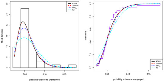
Figure 9. The fitted plots for the second dataset.

Figure 10 shows plots of PLL functions for the parameters $\mu$ and $\sigma$ based on the second dataset. From this figure, we see that the likelihood equations have unique solutions for the MLEs.

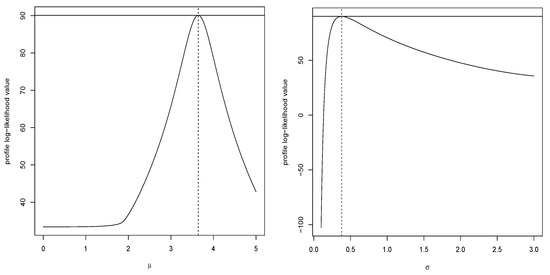
Figure 10. The plots of the PLL functions for the second dataset.

7.2. The Quantile Modeling Application of the Reading Accuracy with the Dyslexia and Intelligence Quotient

Here, a real data application is given in order to see the applicability of the newly defined regression model. We compare its results with the unit Weibull quantile regression model [30]. The quantile parameter u has been taken as 0.5 to model the median for regression models. The pdf of the unit Weibull quantile distribution is given by

$$f(y,\alpha ,\mu )=\frac{\alpha log\left(0.5\right)}{ylog\eta }{\left(\frac{logy}{log\eta }\right)}^{\alpha -1}0.5^{{\left(logy/log\eta \right)}^{\alpha }},y\in (0,1),$$

where $\eta \in (0,1)$ is the median and $\alpha >0$ is the shape parameter. The dataset consists of the reading accuracy for nondyslexic and dyslexic Australian children and contains 44 observations on 3 variables. The variable of interest is accuracy providing the scores on a test of reading accuracy taken by 44 children, which is predicted by the two regressors: dyslexia and nonverbal intelligence quotient (IQ). The dataset has been collected by [41], and analyzed by [42,43] via the beta regression modeling based on the data mean modeling. It is noticed that the original reading accuracy score has been transformed by [43] so that accuracy is in the open unit interval. Further, this dataset can be found easily via betareg function [42] in the R software.

The aim is to associate the reading accuracy values $\left(y\right)$ with covariates. The response variable and covariates are:

• y: reading score;
• $x_1$: Is the child dyslexic? (0 for no, 1 for yes);
• $x_2$: nonverbal intelligence quotient (IQ, converted to z scores).

The regression model based on ${\eta }_i$ is given by

$$\mathrm{logit}\left({\eta }_i\right)={\beta }_0+{\beta }_1{x}_{i1}+{\beta }_2{x}_{i2},i=1,2,\dots ,44,$$

where ${\eta }_i$ denotes the median for the unit Weibull and $EASHN$ models.

The results of the $EASHN$ and unit Weibull regression models with model selection criteria are given in Table 4. As seen from the values of AIC and BIC statistics, the proposed regression model has lower values than those of the unit Weibull regression model. So, one can say that the $EASHN$ regression model exhibits better modeling ability than the unit Weibull regression model. Additionally, according to the estimated parameters of the $EASHN$ regression model, the parameters ${\beta }_1$ and ${\beta }_2$ have been seen statistically significant at any usual level. Hence, it is concluded that, when IQ increases, the reading accuracy increases also. However, the reading accuracy of the children with no dyslexia is higher than those of the children with dyslexia as expected.

Table 4. The results of the $EASHN$ and unit Weibull regression models with model selection criteria.

Parameters	EASHN			Unit-Weibull
	Estimate	SE	p-Value	Estimate	SE	p-Value
${\beta }_0$	2.2810	0.0025	<0.001	2.4045	0.2589	<0.001
${\beta }_1$	−1.0490	0.0028	<0.001	−1.3362	0.3751	0.0003
${\beta }_2$	0.5918	0.00001	<0.001	0.4837	0.2453	0.0486
$\alpha$	0.1260	0.00001	<0.001	0.9795	0.1193	<0.001
ℓ	37.9466			37.3185
AIC	−67.8934			−66.6369
BIC	−60.7566			−59.5001

Figure 11 and Figure 12 display the QQ plots of the randomized quantile residuals and PP plot of the Cox-Snell residuals for both regression models, respectively. These figures indicate that the fit of the $EASHN$ regression model is better than the one of the unit Weibull model.

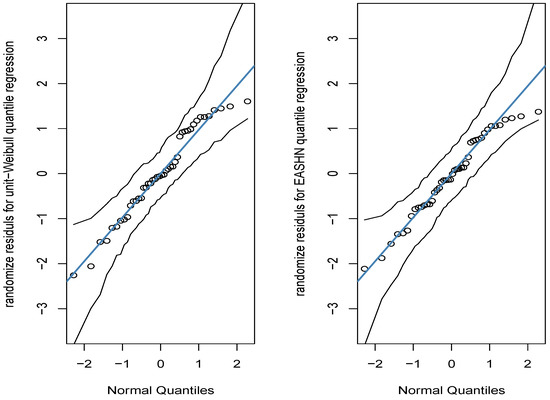
Figure 11. The QQ plot of the randomized quantile residuals.

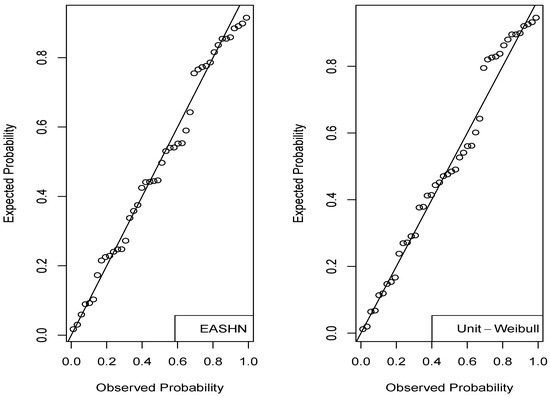
Figure 12. The PP plots of the Cox-Snell residuals based on the regression application.

Since the randomized quantile residuals have standard normal distributions, one may see whether they fit this corresponding distribution. The KS, $A^{*}$ and $W^{*}$ results are given in Table 5. It is clear that the results based on the $EASHN$ quantile regression model of the randomized quantile residuals are more suitable than those of the unit Weibull regression model.

Table 5. The goodness-of-fit results of the randomized quantile residuals for the regression models.

Models	KS	p-Value	${\mathit{A}}^{*}$	p-Value	${\mathit{W}}^{*}$	p-Value
EASHN	0.0849	0.9093	0.4211	0.8267	0.0502	0.8775
Unit-Weibull	0.1159	0.5955	0.4989	0.7470	0.0720	0.7419

8. Conclusions

We define a new unit model, called “arcsech” normal distribution, in order to model percentage, proportion and rate measurements. The idea is to take advantage of the hyperbolic arcsecant function to transpose the modeling capacities of the normal distribution for the processing of data defined on the unit interval. We investigate general structural properties of the new distribution. The model parameters are estimated by six different methods. The simulation studies are performed to see the performances of these estimates. The empirical findings indicate that the proposed model provides better fits than the well-known unit probability distributions in the literature for both its univariate data modeling and its regression modeling. It is hoped that the new distribution will attract attention in the other disciplines.

References

- Johnson, N.L. Systems of frequency curves generated by methods of translation. Biometrika 1949, 36, 149–176. [Google Scholar] [CrossRef]
- Topp, C.W.; Leone, F.C. A family of J-shaped frequency functions. J. Am. Stat. Assoc. 1955, 50, 209–219. [Google Scholar] [CrossRef]
- Kumaraswamy, P. A generalized probability density function for double-bounded random processes. J. Hydrol. 1980, 46, 79–88. [Google Scholar] [CrossRef]
- Van Dorp, J.R.; Kotz, S. The standard two-sided power distribution and its properties: With applications in financial engineering. Am. Stat. 2002, 56, 90–99. [Google Scholar] [CrossRef]
- Gómez-Déniz, E.; Sordo, M.A.; Calderín-Ojeda, E. The log–Lindley distribution as an alternative to the beta regression model with applications in insurance. Insur. Math. Econ. 2014, 54, 49–57. [Google Scholar] [CrossRef]
- Altun, E.; Hamedani, G.G. The log-xgamma distribution with inference and application. J. Soc. Fr. Stat. 2018, 159, 40–55. [Google Scholar]
- Mazucheli, J.; Menezes, A.F.; Dey, S. The unit-Birnbaum-Saunders distribution with applications. Chil. J. Stat. 2018, 9, 47–57. [Google Scholar]
- Mazucheli, J.; Menezes, A.F.B.; Ghitany, M.E. The unit-Weibull distribution and associated inference. J. Appl. Probab. Stat. 2018, 13, 1–22. [Google Scholar]
- Mazucheli, J.; Menezes, A.F.B.; Chakraborty, S. On the one parameter unit-Lindley distribution and its associated regression model for proportion data. J. Appl. Stat. 2019, 46, 700–714. [Google Scholar] [CrossRef]
- Ghitany, M.E.; Mazucheli, J.; Menezes, A.F.B.; Alqallaf, F. The unit-inverse Gaussian distribution: A new alternative to two-parameter distributions on the unit interval. Commun. Stat. Theory Methods 2019, 48, 3423–3438. [Google Scholar] [CrossRef]
- Mazucheli, J.; Menezes, A.F.; Dey, S. Unit-Gompertz distribution with applications. Statistica 2019, 79, 25–43. [Google Scholar]
- Altun, E. The log-weighted exponential regression model: Alternative to the beta regression model. Commun. Stat. Theory Methods 2021. [Google Scholar] [CrossRef]
- Altun, E.; Cordeiro, G.M. The unit-improved second-degree Lindley distribution: Inference and regression modeling. Comput. Stat. 2020, 35, 259–279. [Google Scholar] [CrossRef]
- Korkmaz, M.Ç. A new heavy-tailed distribution defined on the bounded interval: The logit slash distribution and its application. J. Appl. Stat. 2020, 47, 2097–2119. [Google Scholar] [CrossRef]
- Korkmaz, M.Ç. The unit generalized half normal distribution: A new bounded distribution with inference and application. Univ. Politeh. Buchar. Sci. Bull. Ser. Appl. Math. Phys. 2020, 82, 133–140. [Google Scholar]
- Gündüz, S.; Korkmaz, M.Ç. A New Unit Distribution Based On The Unbounded Johnson Distribution Rule: The Unit Johnson SU Distribution. Pak. J. Stat. Oper. Res. 2020, 16, 471–490. [Google Scholar] [CrossRef]
- Figueroa-Zu, J.I.; Niklitschek-Soto, S.A.; Leiva, V.; Liu, S. Modeling heavy-tailed bounded data by the trapezoidal beta distribution with applications. Revstat 2021. Available online: https://www.ine.pt/revstat/pdf/ModelingBoundedDataWithHeavyTails.pdf (accessed on 10 January 2021).
- Bantan, R.A.R.; Chesneau, C.; Jamal, F.; Elgarhy, M.; Tahir, M.H.; Aqib, A.; Zubair, M.; Anam, S. Some new facts about the unit-Rayleigh distribution with applications. Mathematics 2020, 8, 1954. [Google Scholar] [CrossRef]
- Koenker, R.; Bassett, G., Jr. Regression quantiles. Econom. J. Econom. Soc. 1978, 46, 33–50. [Google Scholar] [CrossRef]
- Fischer, M.J. Generalized Hyperbolic Secant Distributions: With Applications to Finance; Springer-Verlag Berlin and Heidelberg GmbH & Co. KG: Berlin, Germany, 2013. [Google Scholar]
- Shaked, M.; Shanthikumar, J.G. Stochastic Orders; Wiley: New York, NY, USA, 2007. [Google Scholar]
- Cheng, R.C.H.; Amin, N.A.K. Maximum Product of Spacings Estimation with Application to the Lognormal Distribution; Math Report; University of Wales Institute of Science and Technology: Cardiff, Wales, 1979; p. 79-1. [Google Scholar]
- Ferrari, S.; Cribari-Neto, F. Beta regression for modelling rates and proportions. J. Appl. Stat. 2004, 31, 799–815. [Google Scholar] [CrossRef]
- Bayes, C.L.; Bazán, J.L.; García, C. A new robust regression model for proportions. Bayesian Anal. 2012, 7, 841–866. [Google Scholar] [CrossRef]
- Kieschnick, R.; McCullough, B.D. Regression analysis of variates observed on (0, 1): Percentages, proportions and fractions. Stat. Model. 2003, 3, 193–213. [Google Scholar] [CrossRef]
- Migliorati, S.; Di Brisco, A.M.; Ongaro, A. A new regression model for bounded responses. Bayesian Anal. 2018, 13, 845–872. [Google Scholar] [CrossRef]
- Galarza, C.E.; Zhang, P.; Lachos, V.H. Logistic quantile regression for bounded outcomes using a family of heavy-tailed distributions. Sankhya B 2020, 1–25. [Google Scholar] [CrossRef]
- Bayes, C.L.; Bazán, J.L.; De Castro, M. A quantile parametric mixed regression model for bounded response variables. Stat. Its Interface 2017, 10, 483–493. [Google Scholar] [CrossRef]
- Mitnik, P.A.; Baek, S. The Kumaraswamy distribution: Median-dispersion re-parameterizations for regression modeling and simulation-based estimation. Stat. Pap. 2013, 54, 177–192. [Google Scholar] [CrossRef]
- Mazucheli, J.; Menezes, A.F.B.; Fernandes, L.B.; de Oliveira, R.P.; Ghitany, M.E. The unit-Weibull distribution as an alternative to the Kumaraswamy distribution for the modeling of quantiles conditional on covariates. J. Appl. Stat. 2020, 47, 954–974. [Google Scholar] [CrossRef]
- Gallardo, D.I.; Gómez-Déniz, E.; Gómez, H.W. Discrete generalized half-normal distribution and its applications in quantile regression. Sort-Stat. Oper. Res. Trans. 2020, 265–284. [Google Scholar] [CrossRef]
- Jodra, P.; Jiménez-Gamero, M.D. A quantile regression model for bounded responses based on the exponential-geometric distribution. Revstat-Stat. J. 2020, 18, 415–436. [Google Scholar]
- Korkmaz, M.Ç.; Chesneau, C.; Korkmaz, Z.S. Transmuted unit Rayleigh quantile regression model: Alternative to beta and Kumaraswamy quantile regression models. Univ. Politeh. Buchar. Sci. Bull. Ser. Appl. Math. Phys. 2021. to appear. [Google Scholar]
- Sánchez, L.; Leiva, V.; Galea, M.; Saulo, H. Birnbaum-Saunders quantile regression models with application to spatial data. Mathematics 2020, 8, 1000. [Google Scholar] [CrossRef]
- Henningsen, A.; Toomet, O. maxLik: A package for maximum likelihood estimation in R. Comput. Stat. 2011, 26, 443–458. [Google Scholar] [CrossRef]
- Dunn, P.K.; Smyth, G.K. Randomized quantile residuals. J. Comput. Graph. Stat. 1996, 5, 236–244. [Google Scholar]
- Cox, D.R.; Snell, E.J. A general definition of residuals. J. R. Stat. Soc. Ser. (Methodol.) 1968, 30, 248–265. [Google Scholar] [CrossRef]
- Murthy, D.P.; Xie, M.; Jiang, R. Weibull Models; John Wiley & Sons: Hoboken, NJ, USA, 2004; Volume 505. [Google Scholar]
- Silva, R.B.; Bourguignon, M.; Dias, C.R.; Cordeiro, G.M. The compound class of extended Weibull power series distributions. Comput. Stat. Data Anal. 2013, 58, 352–367. [Google Scholar] [CrossRef]
- Genç, A.A.; Korkmaz, M.Ç.; Kus, C. The Beta Moyal-Slash Distribution. J. Selçuk Univ. Nat. Appl. Sci. 2014, 3, 88–104. [Google Scholar]
- Pammer, K.; Kevan, A. The Contribution of Visual Sensitivity, Phonological Processing and Non-Verbal IQ to Children’s Reading; The Australian National University: Canberra, Australia, 2004; Unpublished manuscript. [Google Scholar]
- Cribari-Neto, F.; Zeileis, A. Beta regression in R. J. Stat. Softw. 2010, 34, 1–24. [Google Scholar] [CrossRef]
- Smithson, M.; Verkuilen, J. A better lemon squeezer? Maximum-likelihood regression with beta-distributed dependent variables. Psychol. Methods 2006, 11, 54. [Google Scholar] [CrossRef]
Publisher’s Note: MDPI stays neutral with regard to jurisdictional claims in published maps and institutional affiliations. |
© 2021 by the authors. Licensee MDPI, Basel, Switzerland. This article is an open access article distributed under the terms and conditions of the Creative Commons Attribution (CC BY) license (http://creativecommons.org/licenses/by/4.0/).