A Family of Skew-Normal Distributions for Modeling Proportions and Rates with Zeros/Ones Excess

Abstract

In this paper, we consider skew-normal distributions for constructing new a distribution which allows us to model proportions and rates with zero/one inflation as an alternative to the inflated beta distributions. The new distribution is a mixture between a Bernoulli distribution for explaining the zero/one excess and a censored skew-normal distribution for the continuous variable. The maximum likelihood method is used for parameter estimation. Observed and expected Fisher information matrices are derived to conduct likelihood-based inference in this new type skew-normal distribution. Given the flexibility of the new distributions, we are able to show, in real data scenarios, the good performance of our proposal.

1. Introduction

The recent statistical literature has experienced an intense research activity on skew distributions. It is due to the fact that many data sets are not fitted well with the normal distribution because of asymmetry and/or kurtosis excess [1]. A natural extension of the normal distribution is the skew-normal (SN) distribution, which has been studied in [2,3,4,5,6,7,8], among other works. Note that the Fisher information matrix of the SN distribution is singular [1].

In order to model random variables that take values with bounded support, the beta distribution has been frequently used [9,10,11,12,13,14,15,16,17]. This type of variables have interesting applications when the bounded support is between zero and one. Additionaly, versions with support between zero and one of other distributions, such as the Birnbaum–Saunders and Weibull distributions [18,19,20], have been proposed. Variables with support between zero and one are studied particularly when modeling proportions and rates (for example, in the study of the proportion of deaths caused by a certain virus in a country, the rate of income spent on taxes, and the proportion of family income spent on food).

Note that some random variables cannot be observed below a certain value (lower detection limit (LDL)) and/or above a certain value (upper detection limit (UDL)), with LDL and UDL being often fixed values. When LDL and/or UDL are present, we say that the random variable is single/doubly-censored distributed [21,22]. Data associated with this type of variables can be described by censored normal distributions [23,24,25,26].

If LDL $=0$ and UDL $=1$, extensions of the beta distribution may be considered to model excess of zeros and/or ones. These extensions used to describe variables into the intervals [0,1], [0,1) or (0,1] have been reported in [27,28,29], which are named zero/one inflated beta (ZOIB) distributions. In order to model inflation at zero and/or one, mixtures distributions have been derived [30,31]. Bernoulli-beta mixture distributions for modeling inflated data at zero/one have been studied in [28]. However, in many situations, the distribution of random variables that take values between zero and one present positive or negative asymmetry and/or kurtosis degrees different from the normal or beta distributions. Subsequently, other distributions than the beta and Bernoulli-beta mixture models are needed.

In order to solve the problem of asymmetry in the data, a transformation can be considered. Nevertheless, such a transformation brings with it problems in the interpretability of the distribution parameters and loss of power in the inference. As an alternative to not transform the data in the case of random variables with positive support, asymmetry to the right, and presence of LDL/UDL, the Birnbaum-Saunders, log-normal (LN), and log-SN (LSN) distributions can be used [30,32,33,34,35,36]. However, these distributions only cover positive asymmetry. Then, the doubly-censored SN (DCSN) distribution may be proposed as an extension of the doubly-censored normal distribution covering negative and positive asymmetry. To the best of our knowledge, no extensions of the SN distribution to describe variables that take values with bounded support and high censoring, as in the case of the intervals [0,1], [0,1) or (0,1], have been reported to date.

The objective of this paper is to propose an alternative approach to deal with data sets in the [0,1] interval. Our approach is a mixture distribution between the Bernoulli and DCSN distributions, which we name the BDCSN distribution in short. Given that the information matrix of the DCSN distribution is singular, such as in the case of the SN distribution, to circumvent this singularity, we define a centered DCSN (CDCSN) distribution [37]. Therefore, our proposal solves the mentioned problems of the existing distributions and its maximum likelihood estimators are well behaved, with regularity conditions being satisfied, since the Fisher information matrix is non-singular in the vicinity of symmetry.

The paper is organized as follows. In Section 2, we present the DCSN distribution and the main results on inference for this distribution. Given that the information matrix of the DCSN distribution is singular, to solve this problem, in Section 3, we define the CDCSN distribution. In this section, the doubly censored log-SN (DCLSN) is also introduced. In Section 4, the DCSN and DCLSN distributions are considered for modeling zero and/or one inflation by using the BDCSN distribution. Parameter estimation is dealt with the maximum likelihood method. The corresponding observed and expected Fisher information matrices are derived and shown to be non-singular. Section 5 evaluates the performance of the maximum likelihood estimators with simulations based on the Monte Carlo method and introduces an algorithm to generate random numbers from the BDCSN distribution. Two real data analyses are considered on Section 6 and Section 7 from where we conclude that the distributions presented in this paper are a good alternative to the ZOIB distributions. The conclusions of this research are provided in Section 8. Mathematical derivations of this work are detailed in the Appendix A. All the numerical calculations were performed by using the R software [38].

2. Doubly-Censored SN Distribution

In this section, we define the DCSN distribution and estimate its parameter with the maximum likelihood method.

A general structure for a skew-symmetric probability density function (PDF) was proposed in [1], which can be written as

$$g(z;\alpha )=2f\left(z\right)F\left(\alpha z\right),z\in \mathbb{R},\alpha \in \mathbb{R},$$

(1)

where f is a symmetric PDF around zero, F is an absolutely continuous cumulative distribution function (CDF) which is symmetric around zero, and $\alpha$ is a shape parameter controlling the asymmetry of the distribution. In (1), if $f=\varphi$ and $F=\Phi$, that is, the PDF and CDF of the standard normal distribution, respectively, the so called SN distribution is obtained with PDF given by

$${\varphi }_{\mathrm{SN}}(z;\alpha )=2\varphi \left(z\right)\Phi \left(\alpha z\right),z\in \mathbb{R},$$

(2)

in which case the notation $Z\sim \mathrm{SN}\left(\alpha \right)$ is used. Observe that the hazard and inverse-hazard functions of the SN distribution are, respectively, stated as

$$h_{\mathrm{SN}}(z;\alpha )=\frac{{\varphi }_{\mathrm{SN}}(z;\alpha )}{1-{\Phi }_{\mathrm{SN}}(z;\alpha )},r_{\mathrm{SN}}(z;\alpha )=\frac{{\varphi }_{\mathrm{SN}}(z;\alpha )}{{\Phi }_{\mathrm{SN}}\left(z\right)},z\in \mathbb{R},$$

(3)

where ${\Phi }_{\mathrm{SN}}(z;\alpha )=\Phi \left(z\right)-2T(z,\alpha )$ is the SN CDF, with T being the Owen function defined as $T(z,\alpha )=(1/\left(2\pi \right)){\int }_0^{\alpha }exp(-z^2(1+u^2)/2)/(1+u^2)\mathrm{d}u,$ and ${\varphi }_{\mathrm{SN}}(z;\alpha )$ is established in (2).

Let $Z\sim \mathrm{SN}\left(\alpha \right)$. Then, a location-scale extension of Z is obtained considering the transformation $X=\xi +\eta Z$, where $\xi \in \mathbb{R}$ is a location parameter and $\eta \in {\mathbb{R}}^{+}$ is a scale parameter. Therefore, from (2), the PDF of X is expressed as

$${\varphi }_{\mathrm{SN}}(x;{\mathit{\theta }}_1)=\frac{2}{\eta }\varphi \left(\frac{x-\xi }{\eta }\right)\Phi \left(\frac{\alpha (x-\xi )}{\eta }\right),x\in \mathbb{R},$$

(4)

where ${\mathit{\theta }}_1={(\xi ,\eta ,\alpha )}^{\top }$. We denote this extension by $X\sim \mathrm{SN}(\xi ,\eta ,\alpha )$. Next, based on the extension defined in (4), we introduce the DCSN distribution.

Definition 1.

Let $(X_1^{*},\dots ,X_n^{*})$ be a random sample of size n, where $X_i^{*}\sim \mathit{SN}(\xi ,\eta ,\alpha )$ and that only values of $X^{*}$ between the constants $c_0$ and $c_2$ are observed, with $c_0$ and $c_2$ being LDL and UDL, respectively. For values of $X^{*}\le c_0$, only the value $c_0$ is reported, while for values of $X^{*}\ge c_2$ only the value $c_2$ is considered. Then, the observed data set $\mathit{x}=(x_1,\dots ,x_n)$ can be written as

$$x_i=\left\{\begin{array}{cc}{c}_0,\hfill & \mathit{if}{x}_i^{*}\le c_0,\hfill \\ x_i^{*},\hfill & \mathit{if}{c}_0<x_i^{*}<c_2,\hfill \\ c_2,\hfill & \mathit{if}{x}_i^{*}\ge c_2,\hfill \end{array}\right.$$

(5)

for $i=1,\dots ,n$. The resulting sample from (5) is said to be drawn from a DCSN population. For $c_0$ and $c_2$, we have that

$$P(X_i=c_0)=P(X_i^{*}\le c_0)={\Phi }_{\mathit{SN}}(z_0;{\mathit{\theta }}_1)$$

and

$$P(X_i=c_2)=P(X_i^{*}\ge c_2)=1-{\Phi }_{\mathit{SN}}(z_2;{\mathit{\theta }}_1),$$

where

$$z_0=\frac{c_0-\xi }{\eta },z_2=\frac{c_2-\xi }{\eta }.$$

(6)

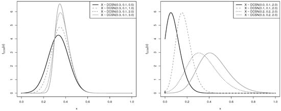
For the continuous part of $c_0<X_i^{*}<c_2$, we consider that $X_i\sim \mathit{SN}(\xi ,\eta ,\alpha )$. In this case, we use the notation $X\sim \mathit{DCSN}(\xi ,\eta ,\alpha ;c_0,c_2)$, with $c_0$ and $c_2$ being fixed. Note that, for $\alpha =0$, the DCSN distribution reduces to the doubly censored normal distribution [23]. Figure 1 provides graphs of PDFs of the DCSN distribution, denoted by $f_{\mathit{DCSN}}$ in this figure.

Figure 1. PDF plots of the DCSN distribution for (left) different values of the parameters $\xi$ and $\eta$; and (right) different values of the parameter $\alpha$; with $c_0=0$ and $c_2=1$.

From Figure 1 (left), note that, as the shape parameter $\alpha$ increases, keeping the other parameters fixed, different shapes of the PDF are obtained. From Figure 1 (right), by keeping $\alpha$ fixed, it is evident that the parameter $\xi$ modifies the location and $\eta$ modifies the scale of the distribution.

Parameter estimation of the DCSN distribution can be performed using the maximum likelihood method. Thus, denoting by ${\sum }_0$, ${\sum }_1$ and ${\sum }_2$ the sums corresponding to $x_i^{*}\le c_0,$$c_0<x_i^{*}<c_2$, and $x_i^{*}\ge c_2$, respectively, the log-likelihood function of ${\mathit{\theta }}_1={(\xi ,\eta ,\alpha )}^{\top }$ for the sample $\mathit{x}=(x_1,\dots ,x_n)$ is given by

$$\begin{array}{ccc}{\ell }_{\mathrm{DCSN}}({\mathit{\theta }}_1;\mathit{x})\hfill & =& \sum _{0}log\left({\Phi }_{\mathrm{SN}}(z_0;{\mathit{\theta }}_1)\right)+\sum _1\left(log\left(2\right)-log\left(\eta \right)+log\left(\varphi \left(z_{1i}\right)\right)+log\left(\Phi \left(\alpha z_{1i}\right)\right)\right)\hfill \\ & & +\sum _{2}log\left(1-{\Phi }_{\mathrm{SN}}\left(z_2;{\mathit{\theta }}_1\right)\right),\hfill \end{array}$$

(7)

where $z_0,z_2$ are defined in (6) and $z_{1i}=\left(x_i-\xi \right)/\eta$. Hence, the score vector defined as the derivative of the log-likelihood function stated in (7) with respect to the distribution parameters has elements $U_{\xi }$, $U_{\eta }$, and $U_{\alpha }$, which are detailed in the Appendix A. The first order conditions or estimating equations for the maximum likelihood method are obtained equating to zero the elements $U_{\xi }$, $U_{\eta }$, and $U_{\alpha }$ of the score vector. The solution of these equations leads to the maximum likelihood estimates of $(\xi ,\eta ,\alpha )$. Notice that these estimating equations must be solved numerically by a nonlinear optimization method, as for example, a quasi-Newton algorithm of Broyden–Fletcher–Goldfarb–Shanno (BFGS) type [39], which is available by the optim function of the R software.

The elements of the observed Fisher information matrix corresponding to the DCSN distribution depend on the second derivatives of the likelihood function with respect to the distribution parameters. These elements are provided in the Appendix A. The expected Fisher information matrix corresponding to the DCSN distribution follows then by taking expectations of the elements of the observed information matrix and multiplying by $n^{-1}$. Subsequently, after intensive algebraic manipulations, the elements of the expected information matrix are obtained and also given in the Appendix A, with 

$$a_{jk}=\mathrm{E}\left(Z^j{\left(\frac{\varphi \left(\alpha z\right)}{\Phi \left(\alpha z\right)}\right)}^k\right),j=1,2,k=0,1,2,$$

(8)

where $a_{jk}$ is defined here due to this is used in Section 4. As mentioned, the Fisher information matrix of the SN distribution is singular [1]. It occurs when $\alpha =0$, since the score of the parameter $\xi$ is $\eta \sqrt{2/\pi }$ times the score of the parameter $\alpha$, producing linear dependence between the corresponding columns of this matrix. Such a singularity is inherited by the Fisher information matrix corresponding to the DCSN distribution, when $\alpha =0$. For this case of $\alpha =0$, a convergence problem exists in the asymptotic inference and the unicity of the corresponding maximum likelihood estimators is not guaranteed.

3. Doubly-Censored Log-SN and Centered SN Distributions

As mentioned, the censored LSN distribution arises as an alternative to not transform the data in the case of random variables with positive support and asymmetry to the right. In this section, we define the DCLSN and centered SN distributions estimating their parameters with the maximum likelihood method.

Recalling that ${\mathit{\theta }}_1={(\xi ,\eta ,\alpha )}^{\top }$, the PDF of a random variable X with LSN distribution is given by

$${\varphi }_{\mathrm{LSN}}(x;{\mathit{\theta }}_1)=\frac{2}{\eta x}\varphi \left(\frac{log\left(x\right)-\xi }{\eta }\right)\Phi \left(\frac{\alpha (log(x)-\xi )}{\eta }\right),x\in {\mathbb{R}}^{+},$$

(9)

where $\xi \in \mathbb{R}$ is a location parameter and $\eta \in {\mathbb{R}}^{+}$ is a scale parameter. Notice that if $\alpha =0$, then the LN distribution is obtained. We denote this extension of the LN distribution as $X\sim \mathrm{LSN}(\xi ,\eta ,\alpha )$. The LSN distribution is required to model data with asymmetry different from that of $Y=log\left(X\right)\sim \mathrm{N}(\xi ,\eta )$, or equivalently, of $X=exp\left(Y\right)\sim \mathrm{LN}(\xi ,\eta )$. Hence, extending the definition of the DCSN distribution to the LSN case, we obtain the DCLSN distribution with parameters $\xi$, $\eta$ and $\alpha$, which is denoted by $\mathrm{DCLSN}(\xi ,\eta ,\alpha ;c_0,c_2)$, with $c_0=\mathrm{LDL}=0$ and $c_2=\mathrm{UDL}=1$, and replacing x by $x+1$ in the DCSN PDF to avoid that the DCLSN PDF is not defined at zero. In this particular case, from the PDF given in (9), the log-likelihood function of ${\mathit{\theta }}_1$ is stated as

$${\ell }_{\mathrm{DCLSN}}({\mathit{\theta }}_1;\mathit{x})=-\sum _{1}log(x+1)+{\ell }_{\mathrm{DCSN}}({\mathit{\theta }}_1;log(x+1)),$$

(10)

where ${\ell }_{\mathrm{DCSN}}$ is the log-likelihood function defined in (7) for the DCSN distribution, with $z_0$ being replaced by $z_0^{\prime }=-\xi /\eta$, $z_{1i}$ by $z_{1i}^{\prime }=(log(x_i+1)-\xi )/\eta$, and $z_2$ by $z_2^{\prime }=(log\left(2\right)-\xi )/\eta$. The score vector and Fisher information matrix associated with the log-likelihood function defined in (10) can be obtained using the score vector and information matrix of the DCSN distribution replacing in the expressions of the Appendix A: (i) $h_{\mathrm{SN}}(z_2;{\mathit{\theta }}_1)$ by $h_{\mathrm{LSN}}(z_2;{\mathit{\theta }}_1)=h_{\mathrm{SN}}\left(z_2^{\prime }\right)/2$, and (ii) $r_{\mathrm{SN}}(z_0;{\mathit{\theta }}_1)$ by $r_{\mathrm{LSN}}(z_0;{\mathit{\theta }}_1)=r_{\mathrm{SN}}\left(z_0^{\prime }\right)$, where $h_{\mathrm{SN}}$ and $r_{\mathrm{SN}}$ are the hazard and inverse hazard functions of the SN distribution, respectively, defined in (3). As mentioned, the Fisher information matrix of the DCSN distribution is singular, inherited from the singularity of the SN distribution. Note that this singularity is also presented in the case of the DCLSN distribution. As also mentioned, a centered parametrization is considered to circumvent such a singularity. Observe that the SN PDF with centered parametrization (CSN in short) is given by

$$\begin{array}{ccc}{\varphi }_{\mathrm{SN}}(x;\mu ,\sigma ,{\gamma }_1)\hfill & =& \frac{2}{\sigma \sqrt{1+c^2{\gamma }_1^{2/3}}}\varphi \left(\frac{1}{\sqrt{1+c^2{\gamma }_1^{2/3}}}\left(\left(\frac{x-\mu }{\sigma }\right)+c{\gamma }_1^{1/3}\right)\right)\hfill \\ & & \times \Phi \left(\frac{c{\gamma }_1^{1/3}}{\sqrt{b^2+c^2(b^2-1){\gamma }_1^{2/3}}\sqrt{1+c^2{\gamma }_1^{2/3}}}\left(\left(\frac{x-\mu }{\sigma }\right)+c{\gamma }_1^{1/3}\right)\right),x\in \mathbb{R},\hfill \end{array}$$

(11)

where $\mu \in \mathbb{R}$, $\sigma \in {\mathbb{R}}^{+}$, $-0.9953<{\gamma }_1<0.9953$, $b=\sqrt{2/\pi }$, and $c={(2/(4-\pi ))}^{1/3}$. The centrality parameters $\mathsf{\mu }$, $\sigma$ and ${\gamma }_1=\sqrt{{\beta }_1}$ represent, as usual, the mean, standard deviation (SD) and coefficient of skewness of X, respectively. In this case, we use the notation $X\sim \mathrm{CSN}(\mu ,\sigma ,{\gamma }_1)$.

Note that the distribution regarding the PDF defined in (11) can be a location-scale distribution denoted by $X\sim \mathrm{SN}(\xi ,\eta ,\alpha )$ considering

$$\xi =\mu -c\sigma {\gamma }_1^{1/3},\eta =\sigma \sqrt{1+c^2{\gamma }_1^{2/3}},\alpha =c{\gamma }_1^{1/3}/\sqrt{b^2+c^2(b^2-1){\gamma }_1^{2/3}}.$$

(12)

By using the relations stated in (12), we parametrize the DCSN distribution to obtain the CDCSN distribution, denoted by $X\sim \mathrm{CDCSN}(\mu ,\sigma ,{\gamma }_1;0,1)$.

Based on the relations established in (12), the observed and expected Fisher information matrices may be obtained for the parameter vector $\mathit{\beta }={(\mu ,\sigma ,{\gamma }_1)}^{\top }$ of the CDCSN distribution using $\mathcal{J}\left(\mathit{\beta }\right)={\mathit{D}}^{\top }\mathcal{J}\left({\mathit{\theta }}_1\right)\mathit{D}$, where $\mathit{D}$ is a matrix containing the derivatives of the vector of parameters ${\mathit{\theta }}_1$ with respect to $\mathit{\beta }$, and $\mathcal{J}\left({\mathit{\theta }}_1\right)$ is the observed Fisher information matrix of the non-centered location-scale SN distribution. Upon regularity conditions [40], $\widehat{\mathit{\beta }}$ is a consistent estimator of $\mathit{\beta }$. In addition, as $n\to \infty$,

$$\sqrt{n}(\widehat{\mathit{\beta }}-\mathit{\beta })\stackrel{\mathrm{d}}{\to }{\mathrm{N}}_3(\mathbf{0},{\mathcal{I}}^{-1}\left(\mathit{\beta }\right)),$$

(13)

where $\mathcal{I}\left(\mathit{\beta }\right)={lim}_{n\to \infty }(1/n)\mathcal{J}\left(\mathit{\beta }\right)$, with $\mathcal{J}\left(\mathit{\beta }\right)$ being the expected Fisher information matrix, and $\stackrel{\mathrm{d}}{\to }$ denotes convergence in distribution to. In summary, $\widehat{\mathit{\beta }}$ is consistent and, from (13), it is asymptotically normal distributed with asymptotic covariance matrix expressed as ${\mathcal{I}}^{-1}\left(\mathit{\beta }\right)$. Note that ${\widehat{\mathcal{J}}}^{-1}\left(\mathit{\beta }\right)$ is a consistent estimator of the asymptotic variance-covariance matrix of $\widehat{\mathit{\beta }}$.

Figure 2 shows some graphical plots of the PDF of the CDCSN distribution with different values for its parameters. The PDF of the CDCSN distribution is denoted by $f_{\mathrm{CDCSN}}$ in this figure. In Figure 2 (left), it is evident that the parameter ${\gamma }_1$ modifies the symmetry of the PDFs, while in Figure 2 (right) the parameters $\mathsf{\mu }$ and $\sigma$ modifies the mean and dispersion of the PDFs, respectively.

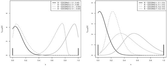
Figure 2. PDF plots of the CDCSN distribution for (left) different values of the parameters $\mathsf{\mu }$ and ${\gamma }_1$; and (right) different values of the parameters $\mathsf{\mu }$ and $\sigma$; with $c_0=0$ and $c_2=1$.

4. The Bernoulli/Doubly-Censored SN Mixture Distribution

As mentioned, when the data set presents detection limits, mixture distributions are often used. In this section, we construct the BDCSN distribution considering the Bernoulli distribution for the discrete mixture variable and the DCSN distribution for the continuous mixture variable.

For the case of proportions, that is, with $c_0=0$ and $c_2=1$, we can construct the mixture of Bernoulli and SN (BSN) distributions. On the one hand, we consider that the zero/one observations are well explained by a Bernoulli distributed variable with parameter $\varsigma$, which we denote by $X\sim \mathrm{Ber}\left(\varsigma \right)$. On the other hand, the remaining observations can be modeled by an SN distribution (or LSN for positive data) with parameters $\xi$, $\eta$ and $\alpha$. The BSN PDF for ${\mathit{\theta }}_2={(p,\varsigma ,{\mathit{\theta }}_1^{\top })}^{\top }={(p,\varsigma ,\xi ,\eta ,\alpha )}^{\top }$ is given by

$$f_{\mathrm{BSN}}(x_i;p,{\mathit{\theta }}_2)=\left\{\begin{array}{cc}p(1-\varsigma ),\hfill & \mathrm{if}{x}_i=0;\hfill \\ (1-p){\displaystyle \frac{{\varphi }_{\mathrm{SN}}(x_i;{\mathit{\theta }}_1)}{{\Phi }_{\mathrm{SN}}(z_2;{\mathit{\theta }}_1)-{\Phi }_{\mathrm{SN}}(z_0;{\mathit{\theta }}_1)}},\hfill & \mathrm{if}0<x_i<1;\hfill \\ p\varsigma ,\hfill & \mathrm{if}{x}_i=1;\hfill \end{array}\right.$$

(14)

where $z_0,z_2$ are defined in (6), $0<p<1$, $0<\varsigma <1$, $\eta >0$, $\alpha >0$ and $\xi \in \mathbb{R}$, with ${\varphi }_{\mathrm{SN}}$ denoting the SN PDF and ${\Phi }_{\mathrm{SN}}$ being the respective CDF. Observe that $\mathrm{P}(X=0)=p(1-\gamma )$ and $\mathrm{P}(X=1)=p\varsigma$. In this case, we use the notation $X\sim \mathrm{BSN}(p,\varsigma ,\xi ,\eta ,\alpha )$. After some algebraic manipulations, the CDF of $X_i$ is stated as

$$F_{\mathrm{BSN}}(x_i;{\mathit{\theta }}_2)=\left\{\begin{array}{cc}0,\hfill & \mathrm{if}{x}_i<0,\hfill \\ p(1-\varsigma ),\hfill & \mathrm{if}{x}_i=0,\hfill \\ p(1-\varsigma )+(1-p){\displaystyle \frac{({\Phi }_{\mathrm{SN}}\left(z_{1i}\right)-{\Phi }_{\mathrm{SN}}(z_0;{\mathit{\theta }}_1))}{({\Phi }_{\mathrm{SN}}(z_2;{\mathit{\theta }}_1)-{\Phi }_{\mathrm{SN}}(z_0;{\mathit{\theta }}_1))}},\hfill & \mathrm{if}0<x_i<1,\hfill \\ 1,\hfill & \mathrm{if}{x}_i\ge 1,\hfill \end{array}\right.$$

(15)

where $z_{1i}=\left(x_i-\xi \right)/\eta$, for $i=1,\dots ,n$, is defined as in (7).

Let $X_1,\dots ,X_n$ be a random sample of size n from $X\sim \mathrm{BSN}(p,\varsigma ,\xi ,\eta ,\alpha )$, with $n_0={\sum }_{i=1}^n{I}_0\left(x\right),$$n_1={\sum }_{i=1}^n{I}_1\left(x\right)$ and $n_{01}={\sum }_{i=1}^n{I}_{(0,1)}\left(x\right),$ where $I_A\left(x\right)$ is an indicator function of $x\in A$. Then, from (14) and (15), the log-likelihood function for ${\mathit{\theta }}_2={(p,\varsigma ,\xi ,\eta ,\alpha )}^{\top }$ based on the data set $\mathit{x}={(x_1,\dots ,x_n)}^{\top }$ is established as

$$\begin{array}{ccc}{\ell }_{\mathrm{BSN}}({\mathit{\theta }}_2;\mathit{x})\hfill & =\hfill & n_{01}log\left(p\right)+(n-n_{01})log(1-p)+n_{1}log\left(\varsigma \right)+n_{0}log(1-\varsigma )\hfill \\ & & +\sum _1\left(log\left(2\right)-log\left(\eta \right)+log\left(\varphi \left(z_{1i}\right)\right)+log\left(\Phi \left(\alpha z_{1i}\right)\right)-log\left({\Phi }_{\mathrm{SN}}(z_2;{\mathit{\theta }}_1)-{\Phi }_{\mathrm{SN}}(z_0;{\mathit{\theta }}_1)\right)\right).\hfill \end{array}$$

(16)

The elements of the score vector obtained from (16) are detailed in the Appendix A. Maximum likelihood estimates of the parameters p, $\varsigma$, $\xi$, $\eta$ and $\alpha$ are the solution to the system which follows by equating the scores to zero. From the first two equations, we obtain an unbiased estimator for p, namely $\widehat{p}=n_{01}/n$, while an estimator for $\varsigma$ is given by $\widehat{\varsigma }=n_1/n_{01}$, corresponding to the proportion of zeros and ones in the sample, as well as the proportions of ones in the subsample of zeros and ones, respectively. The solution to the remaining three parameters can obtained from the last three equations using iterative methods.

The expected Fisher information matrix corresponding to the BSN distribution is derived next. Considering the quantities $a_{kj}$ defined similarly as in (8), with $x\in (0,1)$, for $k=0,1,2$ and $j=1,2$, with ${\theta }_1=p$, ${\theta }_2=\varsigma$, ${\theta }_3=\xi$, ${\theta }_4=\eta$ and ${\theta }_5=\alpha$, we have that the elements of the expected Fisher information matrix, denoted by $k_{{\theta }_r{\theta }_p}=n^{-1}\mathrm{E}(-{\partial }^2\ell ({\mathit{\theta }}_2;\mathit{x})/\partial {\theta }_r\partial {\theta }_s)$, for $r,s=1,2,3,4,5$, are defined as $k_{pp}$, $k_{\varsigma \varsigma }$, $k_{\xi p}$, $k_{\xi \xi }$, $k_{\eta \xi }$, $k_{\eta \eta }$, $k_{\alpha \xi }$, $k_{\alpha \eta }$, $k_{\alpha \alpha }$, and detailed in the Appendix A. Thus, the expected Fisher information matrix for ${\mathit{\theta }}_2={(p,\varsigma ,\xi ,\eta ,\alpha )}^{\top }$ is given by

$$\mathit{K}\left({\mathit{\theta }}_2\right)=(1-p)\left(\begin{array}{ccccc}\frac{1}{p{(1-p)}^2}& 0& 0& 0& 0\\ 0& \frac{p}{\varsigma (1-\varsigma )(1-p)}& 0& 0& 0\\ 0& 0& k_{\xi \xi }& k_{\xi \eta }& k_{\xi \alpha }\\ 0& 0& k_{\xi \eta }& k_{\eta \eta }& k_{\eta \alpha }\\ 0& 0& k_{\xi \alpha }& k_{\eta \alpha }& k_{\alpha \alpha }\end{array}\right).$$

(17)

Notice from (17) that the set of parameters for the discrete components ${(p,\varsigma )}^{\top }$ and the continuous components ${(\xi ,\eta ,\alpha )}^{\top }$ are mutually orthogonal. Therefore, the expected Fisher information matrix can be written as $\mathit{K}\left(\mathit{\theta }\right)=\mathrm{diag}({\mathit{K}}_{p,\varsigma },{\mathit{K}}_{\xi ,\eta ,\alpha }),$ where ${\mathit{K}}_{p,\varsigma }=\mathrm{diag}(1/\left(p\right(1-p\left)\right),p/\left(\varsigma \right(1-\varsigma \left)\right)),$ that is, we have block orthogonality. One of the advantages of this orthogonality is that the corresponding parameters may be estimated separately. Estimation methods were discussed in [36] when there is orthogonality in relation to a partition of interest. Moreover, maximum likelihood estimators are independent asymptotically.

Note that the parameterization ${\delta }_1=p\varsigma$ and ${\delta }_0=p(1-\varsigma )=p-{\delta }_1$ in the BSN distribution leads to the BDCSN distribution, for ${\mathit{\theta }}_3={({\delta }_0,{\delta }_1,{\mathit{\theta }}_1^{\top })}^{\top }={({\delta }_0,{\delta }_1,\xi ,\eta ,\alpha )}^{\top }$, with PDF being defined as

$$f_{\mathrm{BDCSN}}(x_i;{\mathit{\theta }}_3)=\left\{\begin{array}{cc}{\delta }_0,\hfill & \mathrm{if}{x}_i=0,\hfill \\ (1-{\delta }_0-{\delta }_1){\displaystyle \frac{{\varphi }_{\mathrm{SN}}(x_i;{\mathit{\theta }}_1)}{{\Phi }_{\mathrm{SN}}(z_2;{\mathit{\theta }}_1)-{\Phi }_{\mathrm{SN}}(z_0;{\mathit{\theta }}_1)}},\hfill & \mathrm{if}0<x_i<1,\hfill \\ {\delta }_1,\hfill & \mathrm{if}{x}_i=1,\hfill \end{array}\right.$$

(18)

where $0<{\delta }_0=\mathrm{P}(X_i=0),{\delta }_1=\mathrm{P}(X_i=1)<1$ and $0<{\delta }_0+{\delta }_1<1$. This is denoted by $X\sim \mathrm{BDCSN}({\delta }_0,{\delta }_1,\xi ,\eta ,\alpha )$.

Figure 3 shows graphical plots of the PDF of the BDCSN distribution with different values for its parameters. In Figure 3 (left), we note that, as the shape parameter $\alpha$ increases, keeping the other parameters fixed, the shapes of the PDF change. In Figure 3 (right), by keeping $\alpha$ fixed, observe that the parameter $\xi$ modifies the location and $\eta$ modifies the scale of the BDCSN distribution. Subsequently, observe that in both figures different values for ${\delta }_0$ and ${\delta }_1$ are used.

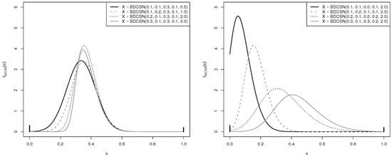
Figure 3. PDF plots of the BDCSN distribution for (left) different values of parameters ${\delta }_0$, ${\delta }_1$ and $\alpha$; and (right) different values of the parameters ${\delta }_0$, ${\delta }_1$, $\xi$ and $\eta$.

From the PDF given in (18), the log-likelihood function of ${\mathit{\theta }}_3={({\delta }_0,{\delta }_1,\xi ,\eta ,\alpha )}^{\top }$ based on the data set $\mathit{x}$ can be written as

$$\begin{array}{ccc}{\ell }_{\mathrm{BDCSN}}({\mathit{\theta }}_3;\mathit{x})\hfill & =\hfill & n_{0}log\left({\delta }_0\right)+n_{1}log\left({\delta }_1\right)+(n-n_{01})log(1-{\delta }_0-{\delta }_1)\hfill \\ & & +\sum _1\left(log\left(2\right)-log\left(\eta \right)+log\left(\varphi \left(z_{1i}\right)\right)+log\left(\Phi \left(\alpha z_{1i}\right)\right)-log({\Phi }_{\mathrm{SN}}(z_2;{\mathit{\theta }}_2)-{\Phi }_{\mathrm{SN}}(z_0;{\mathit{\theta }}_2))\right).\hfill \end{array}$$

(19)

Therefore, from (19), the elements of the score vector for ${\delta }_0$ and ${\delta }_1$ are $U_{{\delta }_0}=n_0/{\delta }_0-(n-n_{01})/(1-{\delta }_0-{\delta }_1)$ and $U_{{\delta }_1}=n_1/{\delta }_1-(n-n_{01})/(1-{\delta }_0-{\delta }_1)$. For $\xi$, $\eta$ and $\alpha$ given by the non-reparametrized distribution, the solution follows using the BFGS algorithm [39]. In addition, ${\widehat{\delta }}_0=n_0/n$ is the proportion of zeros in the sample, and ${\widehat{\delta }}_1=n_1/n$ is the proportion of ones in the sample. For this distribution, its Fisher information matrix can be written as $\mathit{K}\left({\mathit{\theta }}_2\right)=\mathrm{diag}({\mathit{K}}_{{\delta }_0,{\delta }_1},{\mathit{K}}_{\xi ,\eta ,\alpha }),$ where the elements of ${\mathit{K}}_{{\delta }_0,{\delta }_1}$ are given by $k_{{\delta }_0{\delta }_0}=(1-{\delta }_1)\left({\delta }_0(1-{\delta }_0-{\delta }_1)\right)$, $k_{{\delta }_1{\delta }_0}=1/(1-{\delta }_0-{\delta }_1)$, and $k_{{\delta }_1{\delta }_1}=(1-{\delta }_0)/\left({\delta }_1(1-{\delta }_0-{\delta }_1)\right).$ Furthermore, the elements of ${\mathit{K}}_{\xi ,\eta ,\alpha }$ are the corresponding elements of $X\sim \mathrm{BSN}(p,\varsigma ,\xi ,\eta ,\alpha )$. Given the orthogonality for the two sets of parameters, their estimates are computed separately.

Next, we present the inflated zero, inflated one and zero/one inflated cases of the BDCSN distribution. For the case of zero inflation $({\delta }_1=0)$ with ${\mathit{\theta }}_4={({\delta }_0,\xi ,\eta ,\alpha )}^{\top }$, its PDF is given by

$$f_{\mathrm{BDCSN}}(x_i;{\delta }_1=0,{\mathit{\theta }}_4)=\left\{\begin{array}{cc}{\delta }_0,\hfill & \mathrm{if}{x}_i=0,\hfill \\ (1-{\delta }_0){\displaystyle \frac{{\varphi }_{\mathrm{SN}}(x_i;{\mathit{\theta }}_1)}{{\Phi }_{\mathrm{SN}}(z_2;{\mathit{\theta }}_1)-{\Phi }_{\mathrm{SN}}(z_0;{\mathit{\theta }}_1)}},\hfill & \mathrm{if}0<x_i\le 1,\hfill \end{array}\right.$$

(20)

where $0<{\delta }_0=\mathrm{P}(X_i=0)<1$. Then, from the PDF stated in (20), the log-likelihood function of ${\mathit{\theta }}_4={({\delta }_0,\xi ,\eta ,\alpha )}^{\top }$ based on the data set $\mathit{x}$ can be written as

$$\begin{array}{ccc}{\ell }_{\mathrm{BDCSN}}({\mathit{\theta }}_4;\mathit{x})\hfill & =\hfill & n_{0}log\left({\delta }_0\right)+(n-n_0)log(1-{\delta }_0))\hfill \\ & & +\sum _1\left(log\left(2\right)-log\left(\eta \right)+log\left(\varphi \left(z_{1i}\right)\right)+log\left(\Phi \left(\alpha z_{1i}\right)\right)-log({\Phi }_{\mathrm{SN}}(z_2;{\mathit{\theta }}_1)-{\Phi }_{\mathrm{SN}}(z_0;{\mathit{\theta }}_1))\right).\hfill \end{array}$$

(21)

Hence, from (21), the score for ${\delta }_0$ is defined as $U_{{\delta }_0}=n_0/{\delta }_0-n-n_0/1-{\delta }_0$. By equating it to zero, we obtain the estimate ${\widehat{\delta }}_0=n_0/n$, that is, the proportion of zeros in the sample. The remaining parameters are estimated similarly as above.

For the case of one inflation $({\delta }_0=0)$ with ${\mathit{\theta }}_5={({\delta }_1,\xi ,\eta ,\alpha )}^{\top }$, its PDF is stated as

$$f_{\mathrm{BDCSN}}(x_i;{\delta }_0=0,{\mathit{\theta }}_5)=\left\{\begin{array}{cc}(1-{\delta }_1){\displaystyle \frac{{\varphi }_{\mathrm{SN}}(x_i;{\mathit{\theta }}_1)}{{\Phi }_{\mathrm{SN}}(z_2;{\mathit{\theta }}_1)-{\Phi }_{\mathrm{SN}}(z_0;{\mathit{\theta }}_1)}},\hfill & \mathrm{if}0\le x_i<1,\hfill \\ {\delta }_1,\hfill & \mathrm{if}{x}_i=1,\hfill \end{array}\right.$$

(22)

where $0<{\delta }_1=\mathrm{P}(X_i=1)<1$. Thus, from the PDF expressed in (22), the log-likelihood function of ${\mathit{\theta }}_5={({\delta }_1,\xi ,\eta ,\alpha )}^{\top }$ considering the data $\mathit{x}$ is established as

$$\begin{array}{ccc}\ell ({\mathit{\theta }}_5;\mathit{x})\hfill & =\hfill & n_{1}log\left({\delta }_1\right)+(n-n_1)log(1-{\delta }_1)\hfill \\ & & +\sum _1\left(log\left(2\right)-log\left(\eta \right)+log\left(\varphi \left(z_{1i}\right)\right)+log\left(\Phi \left(\alpha z_{1i}\right)\right)-log({\Phi }_{\mathrm{SN}}(z_2;{\mathit{\theta }}_1)-{\Phi }_{\mathrm{SN}}(z_0;{\mathit{\theta }}_1))\right).\hfill \end{array}$$

(23)

From (23), we reach the score for ${\delta }_1$ as $U_{{\delta }_1}=n_1/{\delta }_1-(n-n_1)/(1-{\delta }_1).$ By equating it to zero, we obtain the estimate ${\widehat{\delta }}_1=n_1/n$, that is, the proportion of ones in the sample. The remaining parameters are estimated as in the previous case.

Now, by considering the PDF given in (18), the BDCSN distribution is obtained, which can be used for fitting positive data with high kurtosis and asymmetry. Then, from the PDF expressed in (18), the log-likelihood function of ${\mathit{\theta }}_3={({\delta }_0,{\delta }_1,{\mathit{\theta }}_1^{\top })}^{\top }={({\delta }_0,{\delta }_1,\xi ,\eta ,\alpha )}^{\top }$ considering the data $\mathit{x}$ is given by

$${\ell }_{\mathrm{BDCSN}}({\mathit{\theta }}_3;\mathit{x})=-\sum _{1}log\left(x_i\right)+{\ell }_{\mathrm{BSN}}({\mathit{\theta }}_3;log\left(\mathit{x}\right)),$$

(24)

where $log\left(\mathit{x}\right)={(log\left(x_1\right),\dots ,log\left(x_n\right))}^{\top }$ and ${\ell }_{\mathrm{BSN}}$ is the log-likelihood function defined in (16) for the BSN distribution, with

$$p=\frac{{\delta }_1}{1-{\delta }_0/{\delta }_1}$$

(25)

and

$$\varsigma =1-\frac{{\delta }_0}{{\delta }_1}.$$

(26)

The score vector and information matrices are easily obtained from (24)–(26), and the previous results.

We denote the mixture between the Bernoulli and CDCSN distributions by $X\sim \mathrm{BCDCSN}({\delta }_0,{\delta }_1,\mu ,\sigma ,{\gamma }_1)$. Note that the Fisher information matrix for the continuous part of the BCDCSN distribution is obtained similarly as for the CDCSN distribution, that is, $\mathcal{J}\left(\mathit{\beta }\right)={\mathit{D}}^{\top }\mathcal{J}\left({\mathit{\theta }}_1\right)\mathit{D}$, and $\mathcal{I}\left(\mathit{\beta }\right)={\mathit{D}}^{\top }{\mathit{K}}_{{\mathit{\theta }}_1}\mathit{D}$.

5. Monte Carlo Simulation Study

In this section, we evaluate the performance of the maximum likelihood estimators with simulations based on the Monte Carlo method. For this simulation study, we consider the BDCSN distribution.

In this Monte Carlo simulation, the true values assumed for the parameters are $\xi =0.2$, $\eta =0.2$ and $\alpha$ = 0.3, whereas that ${\delta }_0\in \{0.1,0.2,0.3\}$ and ${\delta }_1\in \{0.1,0.2\}$. The sample sizes considered are $n\in \{25,50,100,500\}$ and the number of Monte Carlo replicates is 5000. In each of these replications, we generate random numbers according to Algorithm 1.

Algorithm 1 Generation of random numbers from the BDCSN distribution.

1: Fix values for ${\delta }_0$, ${\delta }_1$, $\xi$, $\eta$, and $\alpha$.

2: Generate values for u from $U\sim \mathrm{Uniform}({\delta }_0,1-{\delta }_1)$.

3: Compute values for x from $$x={\Phi }_{\mathrm{SN}}^{-1}\left(q_0+\frac{u-{\delta }_0}{1-{\delta }_0-{\delta }_1}(q_1-q_0),\xi ,\eta ,\alpha \right),$$ where $q_0=\Phi (0,\xi ,\eta ,\alpha )$, $q_1=\Phi (1,\xi ,\eta ,\alpha )$ and ${\Phi }_{\mathrm{SN}}^{-1}$ is the quantile function of the SN distribution.

4: Repeat steps 2–3 until the required numbers of data (n) is completed.

For each parameter and sample size, we report the empirical mean, variance, bias and root of the mean squared error (RMSE) of the maximum likelihood estimators in Table 1. From this table, in general, note that, as the sample size increases, both the bias and RMSE decrease, as expected. These results empirically shows the good performance of the maximum likelihood estimators for the BDCSN distribution parameters.

Table 1. Empirical mean, variance, bias and RMSE for the indicated estimator and n with simulated data.

			$\mathit{n}=\mathbf{30}$				$\mathit{n}=\mathbf{50}$				$\mathit{n}=\mathbf{100}$				$\mathit{n}=\mathbf{500}$
${\mathit{\delta }}_{\mathbf{0}}$	${\mathit{\delta }}_{\mathbf{1}}$	True Value	Mean	Variance	Bias	RMSE	Mean	Variance	Bias	RMSE	Mean	Variance	Bias	RMSE	Mean	Variance	Bias	RMSE
0.1	0.1	$\xi$ = 0.2	0.21148	0.00110	0.01148	0.03513	0.20632	0.00137	0.00632	0.03755	0.20642	0.00124	0.00642	0.03578	0.20976	0.00035	0.00976	0.02109
0.1	0.1	$\eta =0.2$	0.18965	0.00057	0.01034	0.02597	0.19227	0.00054	0.00773	0.02459	0.19269	0.00053	0.00730	0.02419	0.19235	0.00018	0.00765	0.01554
0.1	0.1	$\alpha$ = 0.3	0.31774	0.01593	0.01774	0.12746	0.35869	0.06063	0.05869	0.25314	0.35355	0.05694	0.05355	0.24457	0.31103	0.00205	0.01103	0.04661
0.1	0.2	$\xi$ = 0.2	0.21323	0.00123	0.01323	0.03752	0.20943	0.00126	0.00943	0.03669	0.20649	0.00142	0.00649	0.03830	0.21034	0.00044	0.01033	0.02345
0.1	0.2	$\eta =0.2$	0.18861	0.00065	0.01138	0.02796	0.19103	0.00052	0.00896	0.02458	0.19247	0.00056	0.00752	0.02489	0.19218	0.00021	0.00781	0.01654
0.1	0.2	$\alpha$ = 0.3	0.30536	0.01117	0.00536	0.10581	0.33359	0.04294	0.03359	0.20994	0.36002	0.06839	0.06002	0.26833	0.30800	0.00443	0.00800	0.06709
0.2	0.1	$\xi$ = 0.2	0.21216	0.00120	0.01216	0.03678	0.20810	0.00126	0.00810	0.03650	0.20556	0.00137	0.00556	0.03754	0.21035	0.00044	0.01035	0.02345
0.2	0.1	$\eta =0.2$	0.18884	0.00066	0.01115	0.02812	0.19139	0.00053	0.00860	0.02460	0.19262	0.00055	0.00737	0.02474	0.19217	0.00021	0.00782	0.01653
0.2	0.1	$\alpha$ = 0.3	0.31271	0.01290	0.01271	0.11430	0.34589	0.05113	0.04589	0.23075	0.36530	0.06428	0.06530	0.26181	0.30776	0.00416	0.00776	0.06501
0.2	0.2	$\xi$ = 0.2	0.21338	0.00143	0.01338	0.04013	0.21185	0.00118	0.01185	0.03633	0.20870	0.00132	0.00870	0.03749	0.21051	0.00049	0.01051	0.02453
0.2	0.2	$\eta =0.2$	0.18768	0.00076	0.01231	0.03026	0.18964	0.00056	0.01035	0.02601	0.19139	0.00052	0.00860	0.02448	0.19200	0.00024	0.00799	0.01732
0.2	0.2	$\alpha$ = 0.3	0.30392	0.00752	0.00392	0.08681	0.31181	0.01922	0.01181	0.13914	0.34616	0.06196	0.04616	0.25316	0.30677	0.00369	0.00677	0.06119
0.3	0.1	$\xi$ = 0.2	0.21337	0.00143	0.01337	0.04018	0.21184	0.00116	0.01184	0.03608	0.20867	0.00134	0.00867	0.03767	0.21049	0.00049	0.01049	0.02467
0.3	0.1	$\eta =0.2$	0.18769	0.00076	0.01230	0.03026	0.18963	0.00056	0.01036	0.02602	0.19141	0.00052	0.00859	0.02447	0.19201	0.00024	0.00798	0.01734
0.3	0.1	$\alpha$ = 0.3	0.30449	0.00951	0.00449	0.09766	0.31186	0.01993	0.01186	0.14167	0.34602	0.05773	0.04602	0.24464	0.30712	0.00439	0.00712	0.06670
0.3	0.2	$\xi$ = 0.2	0.21357	0.00172	0.01357	0.04367	0.21245	0.00135	0.01245	0.03886	0.21158	0.00115	0.01158	0.03577	0.21117	0.00057	0.01117	0.02648
0.3	0.2	$\eta =0.2$	0.18669	0.00090	0.01330	0.03296	0.18889	0.00069	0.01110	0.02851	0.18981	0.00055	0.01019	0.02555	0.19163	0.00029	0.00836	0.01902
0.3	0.2	$\alpha$ = 0.3	0.30823	0.00996	0.00824	0.10013	0.30489	0.00961	0.00489	0.09818	0.31686	0.02287	0.01687	0.15217	0.30325	0.00537	0.00325	0.07338

6. Real Data Application 1

In this section, we illustrate the usefulness of the CDCSN and BDCSN distributions considering a first application to a real data set. We name this data set as “death”, which corresponds to the proportions of unexplained infant deaths in 5561 Brazilian counties. The data set is available for downloading at https://datasus.saude.gov.br and contains 3367 zeros (explained deaths) and 174 ones (unexplained deaths).

Table 2 provides descriptive statistics for the death data (uncensored), including central tendency statistics, SD, coefficients of variation (CV), skewness (CS) and kurtosis (CK). From this table, note the presence of skewness and kurtosis in the distribution of the data; see also Figure 4 (left), which depicts the histogram with boxplot revealing the distributional behavior.

Table 2. Descriptive statistics of the death data.

Minimum	Median	Mean	SD	CV	CS	CK	Maximum
0.003	0.250	0.292	0.216	73.892	0.811	−0.206	0.941

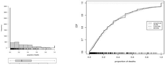
Figure 4. (left) Histogram of the proportion of deaths and (right) empirical CDF (solid line in stairs), and estimated CDF of the CDCSN (dashed and doted line), BDCSN (dashed line), and ZOIB (doted line) distributions, with death data.

In order to compare our distributions with a standard competitor, the ZOIB distribution [28] is considered and denoted by ZOIB $({\delta }_0,{\delta }_1,\mu ,\sigma )$. To estimate the ZOIB distribution parameters, the  GAMLSS package of the R software is used. Then, we fit the CDCSN, BDCSN and ZOIB distributions by using the maximum likelihood method to estimate their parameters based on the  sn package [41] and its selm and dp2cp functions. The  optim function of the R software and the BFGS algorithm are used for this estimation. As starting values to initiate the algorithm, we use the moment estimates proposed in [5]. Table 3 provides the maximum likelihood estimates for the considered distributions. In addition, for  the CDCSN distribution, using the corresponding estimated CDF, the estimated proportions of censored observations are 0.6039 (zeros) and 0.0272 (ones), respectively, whereas the corresponding empirical percentages are 0.6055 and 0.0313, revealing the model fits the data well. Figure 4 shows the estimated CDF of the ZOIB, CDCSN and BDCSN distributions indicating their good fit to the data.

Table 3. Maximum likelihood estimates for ZOIB, CDCSN and BDCSN parameters (with approximate standard errors in parentheses) and information criteria and log-likelihood values, with death data.

Estimate	ZOIB	CDCSN	BDCSN
$\widehat{\mu }$	0.2974 (0.0043)	−0.0691 (0.0217)	0.1965 (0.0039)
$\widehat{\sigma }$	0.4562 (0.0050)	0.4448 (0.0248)	0.1818 (0.0040)
${\widehat{\gamma }}_1$	–	0.6374 (0.1900)	0.9905 (0.0023)
${\widehat{\delta }}_0$	0.6055 (0.0066)	–	0.6055 (0.0066)
${\widehat{\delta }}_1$	0.0313 (0.0023)	–	0.0313 (0.0023)
AIC	7464.2	7615.6	7455.7
BIC	7498.7	7635.5	7488.8
CAIC	7466.2	7617.6	7457.7
$\ell \left(\widehat{\mathit{\theta }}\right)$	−3728.1	−3804.8	−3722.9

We can numerically compare the distributions studied in this application while using the Akaike information criterion (AIC), the Schwarz Bayesian information criterion (BIC), and corrected Akaike information criterion (CAIC) [42]. The AIC, BIC, and CAIC are given, respectively, by

$$\mathrm{AIC}=-2\ell \left(\widehat{\mathit{\theta }}\right)+2d,\mathrm{BIC}=-2\ell \left(\widehat{\mathit{\theta }}\right)+dlog\left(n\right),\mathrm{CAIC}=-2\ell \left(\widehat{\mathit{\theta }}\right)+2d+\frac{2d^2+2d}{n-d-1},$$

(27)

where $\ell \left(\widehat{\mathit{\theta }}\right)$ is the log-likelihood function for $\mathit{\theta }$, associated with the underlying distribution, evaluated at $\mathit{\theta }=\widehat{\mathit{\theta }}$, d is the dimension of the parameter space, and n is the size of the data set. All of these criteria are based on the log-likelihood function and penalize the distribution with more parameters. A distribution whose information criterion has a smaller value is better [43]. The log-likelihood, AIC, BIC and CAIC values computed according to expressions given in (27), for the distributions studied in this application, are presented in Table 3. From this table, observe that the BDCSN distribution has a better agreement with the death data. Additionally, in order to compare the CDCSN and BDCSN distributions against the ZOIB distribution, we use the Voung test [44], with its statistic being a distance between two distributions measured in terms of the Kullback–Liebler criterion [45]. Then, when comparing the BDCSN and ZOIB distributions, the p-value of the Voung value is <0.001, providing a highly significant evidence in favor that the BDCSN distribution fits the death data better than the ZOIB distribution. Similarly, the Voung p-value is <0.001 when comparing the BDCSN and DCSN distributions in favor of the BDCSN distribution, but the ZOIB distribution fits the data better than the CDCSN distribution. These results demonstrate the fact that the BDCSN distribution is a viable option to the ZOIB distribution to model the death data.

7. Real Data Application 2

In this section, in order to provide evidence that the distributions proposed in this paper fit different types of data, we analyze a second data set corresponding to the cable TV penetration in USA. These data were collected by the Federal Communications Commission (FCC) by means of questionnaires applied to cable community units, which are individual franchise areas. These questionnaires supplied data on prices, costs and cable operator background; see details of the questionnaire in Appendix E of [46]. We name this data set as “FCC” and corresponds to 282 individual areas franchising cable TV; see [12] for an analysis of these data. For FCC data, we study the proportion of subscribers going for additional canals.

The FCC data set contains 62 zeros, with the clump-at-zero in the histogram representing 21.98% of the data; see bold line in the histogram of Figure 5 (left). Therefore, we note that this variable has excess of zeros. Table 4 provides descriptive statistics for the data set in study (uncensored), including median, mean, SD, CV, CS and CK. From this table, note the presence of skewness and kurtosis in the distribution of the data; see also Figure 5 (left), which depicts the histogram with boxplot revealing the behavior of the data.

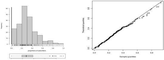
Figure 5. (left) Histogram for the proportion of subscribers and (right) QQ plot for the BDCSN distribution with FCC data.

Table 4. Descriptive statistics of the FCC data.

Minimum	Median	Mean	SD	CV	CS	CK	Maximum
0.007	0.269	0.305	0.18	59.034	0.918	0.969	0.927

We adjust four distributions to the FCC data: (i) the CSN distribution censored at $X=0$, (ii) the BDCSN distribution, (iii) the ZOIB distribution (with no ones), and (iv) the normal distribution censored at $X=0$. The maximum likelihood estimates for the parameters of these four distributions, with approximate standard errors in parentheses, are reported in Table 5. The log-likelihood, AIC, BIC and CAIC values computed according to expressions given in (27), for the distributions studied in this second application, are also presented in Table 5. From this table, observe that the BDCSN distribution has a better agreement with the FCC data. Additionally, when comparing the BDCSN and ZOIB distributions with the Vuong test, the corresponding p-value is 0.2124 indicating a statistically non-significant difference and demonstrating that both distributions are good alternatives to model these data. When comparing the BDCSN and censored normal distributions, the Voung p-value is <0.001 favoring the BDCSN distribution, which also occurs if we compare the CSN and BDCSN distributions. In summary, the BDCSN distribution seems to be a good alternative of modeling for the FCC data, which can be visually corroborated by Figure 5 (right), where the empirical quantile versus theoretical quantile (QQ) plot for the BDCSN distribution is depicted.

Table 5. Maximum likelihood estimates for ZOIB, censored normal, CSN and BDCSN distributions (with approximate standard errors in parentheses) and information criteria and log-likelihood values, with FCC data.

Estimate	ZOIB	Normal	CSN	BDCSN
$\widehat{\mu }$	0.3080 (0.0140)	0.2069 (0.0153)	0.2110 (0.0153)	0.2952 (0.0156)
$\widehat{\sigma }$	5.3239 (0.0004)	0.2487 (0.0125)	0.2455 (0.0129)	0.1873 (0.0121)
$\widehat{\varsigma }$	–	–	0.4046 (0.1937)	0.5750 (0.1644)
${\widehat{\delta }}_0$	0.2198 (0.0006)	–	–	0.2198 (0.0006)
AIC	144.748	142.258	150.278	135.197
BIC	155.674	149.542	161.205	149.765
CAIC	146.893	144.344	152.423	137.415
$\ell \left(\widehat{\mathit{\theta }}\right)$	−69.374	−69.127	−72.139	−63.599

8. Conclusions and Future Research

This paper reported the following findings:

(i)

By using skew-normal distributions, we have proposed a new family of distributions which are an alternative to the beta distribution when an excess zeros and/or one inflation is present.

(ii)

The parameters of the distributions were estimated by the maximum likelihood method.

(iii)

The expected and observed Fisher information matrices associated with the new family of distributions were derived, and an parameterization was proposed to circumvent a singularity problem in these matrices, which is inherited from the classical skew-normal distribution.

(iv)

The Fisher information matrix related to the new mixture distribution obtained in this study resulted to be block ortogonal, facilitating the estimation of parameters and doing it separately in two groups with respect to the discrete and continuous parts of this mixture, respectively.

(v)

An algorithm to generate random numbers from the new family of distributions derived in this study was proposed and implemented.

(vi)

Monte Carlo simulations based on the new family of distributions proposed in this research were provided to detect performance of the maximum likelihood estimators of their parameters.

(vii)

Examples with two real data sets were performed to illustrate the potential applications with the new family of distributions based on the skew-normal distribution proposed in the paper. In addition, we compare the new distributions to their natural competitors, corresponding to the beta and normal distributions, showing their convenience.

In summary, we have proposed new distributions based on the skew-normal distribution, which allows us to model proportions and rates with zero/one inflation as an alternative to the inflated beta distributions. We used the maximum likelihood method for parameter estimation and the observed and expected Fisher information matrices were derived to conduct likelihood-based inference. Numerical studies with simulated and real data were performed to show the good empirical behavior of the estimators and to illustrate potential applications. Therefore, this investigation may be a knowledge addition to the tool-kit of diverse practitioners, including biometrists, engineers, statisticians, and data scientists.

Some open problems that arose from the present investigation are the following:

(i)

Parameter estimates of censored distributions are more efficient than when censorship is not considered. Indeed, if censored cases are present and a non-censored distribution is used, evidently it is not possible to estimate the variance of the censored part. However, if censored distributions are utilized in this case, such a variance may be estimated from the data. For more details, see page 199 in [47]. Subsequently, the study of asymptotic efficiency bounds in the new family of distributions proposed in the present investigation is an issue of interest; see details in [48]. In addition, asymptotic behavior and performance of maximum likelihood estimators in more complex statistical models can be studied in [49,50].

(ii)

The use of covariates when modeling a doubly-censored response with support in [0, 1] following the new family of distributions is of interest. In this case, type Tobit models can be considered as benchmark to compare the new regression models. Specifically, when studying a doubly-censored response in [0, 1] through a linear predictor which includes covariates, the number of observations below $c_0$ and/or above $c_2$ can be modeled by a Bernoulli distribution with a logit link function and polychotomous response. Given the possible orthogonality in the information matrix, the parameters of this model of two parts can be estimated separately. Refs. [30,36] discussed estimation methods for the regression parameters in a similar context under a mixture structure.

(iii)

An extension of the present study to the multivariate case is also of practical relevance [50,51,52].

(iv)

Incorporation of temporal, spatial, functional, and quantile regression structures in the modeling, as well as errors-in-variables, and PLS regression, are also of interest [53,54,55,56,57,58,59,60,61].

(v)

The derivation of diagnostic techniques to detect potential influential cases are needed, which are an important tool to be used in all statistical modeling [7,58,62].

(vi)

Robust estimation methods when outliers are present into the data set can be used [63].

(vii)

Applications of the new methodology derived here can be of interest in diverse areas [64].

Therefore, the proposed results in this study promote new challenges and offer an open door to explore other theoretical and numerical issues. Research on these and other issues are in progress and their findings will be reported in future articles.

Appendix A.1. Doubly-Censored SN Distribution

The elements of the score vector for the DCSN distribution are expressed as

$$\begin{array}{ccc}{U}_{\xi }\hfill & =& -\frac{1}{\eta }\sum _0{r}_{\mathrm{SN}}\left(z_0\right)+\frac{1}{\eta }\sum _1\left(z_{1i}-\alpha r_{1i}\right)+\frac{1}{\eta }\sum _2{h}_{\mathrm{SN}}\left(z_2\right),\hfill \\ U_{\eta }\hfill & =& -\frac{1}{\eta }\sum _0{z}_0{r}_{\mathrm{SN}}\left(z_0\right)+\frac{1}{\eta }\sum _1\left(z_{1i}^2-\alpha z_{1i}{r}_{1i}-1\right)+\frac{1}{\eta }\sum _2{z}_2{h}_{\mathrm{SN}}\left(z_2\right),\hfill \\ U_{\alpha }\hfill & =& -\sqrt{\frac{2}{\pi }}\frac{1}{(1+{\alpha }^2)}\left(\sum _0\frac{\varphi \left(\sqrt{1+{\alpha }^2}\right)}{{\Phi }_{\mathrm{SN}}\left(z_0\right)}-\sum _2\frac{\varphi \left(\sqrt{1+{\alpha }^2}{z}_2\right)}{(1-{\Phi }_{\mathrm{SN}}\left(z_2\right))}\right)+\sum _1{z}_{1i}\frac{\varphi \left(\alpha z_{1i}\right)}{\Phi \left(\alpha z_{1i}\right)},\hfill \end{array}$$

with $z_0,z_2,z_{1i}$ being defined in (7), $h_{\mathrm{SN}},r_{\mathrm{SN}}$ being stated in (3), and $r_{1i}=\varphi \left(z_{1i}\right)/\Phi \left(z_{1i}\right)$.

The elements of the observed information matrix corresponding to the DCSN distribution can be written as

$$\begin{array}{ccc}{j}_{\xi \xi }\hfill & =& \frac{1}{{\eta }^2}\sum _0{r}_{\mathrm{SN}}\left(z_0\right)\left(z_0+r_{\mathrm{SN}}\left(z_0\right)-\sqrt{\frac{2}{\pi }}\frac{\alpha \varphi \left(\sqrt{1+{\alpha }^2}{z}_0\right)}{{\varphi }_{\mathrm{SN}}\left(z_0\right)}\right)+\frac{1}{{\eta }^2}\sum _1(1+{\alpha }^3{z}_{1i}{r}_{1i}+{\alpha }^2{r}_{1i}^2)\hfill \\ & & +\frac{1}{{\eta }^2}\sum _2{h}_{\mathrm{SN}}\left(z_2\right)\left(h_{\mathrm{SN}}\left(z_2\right)-z_2+\sqrt{\frac{2}{\pi }}\frac{\alpha \varphi \left(\sqrt{1+{\alpha }^2}{z}_2\right)}{{\varphi }_{\mathrm{SN}}\left(z_2\right)}\right),\hfill \\ j_{\eta \xi }\hfill & =& \frac{1}{{\eta }^2}\sum _0{r}_{\mathrm{SN}}\left(z_0\right)\left(z_0^2-1+z_0{r}_{\mathrm{SN}}\left(z_0\right)-\sqrt{\frac{2}{\pi }}\alpha z_0\frac{\varphi \left(\sqrt{1+{\alpha }^2}{z}_0\right)}{{\varphi }_{\mathrm{SN}}\left(z_0\right)}-1\right)\hfill \\ \hfill & \hfill & +\frac{1}{{\eta }^2}\sum _1(2z_{1i}-\alpha r_{1i}+{\alpha }^3{z}_{1i}^2{r}_{1i}+{\alpha }^2{z}_{1i}{r}_{1i}^2)\hfill \\ \hfill & \hfill & +\frac{1}{{\eta }^2}\sum _2{h}_{\mathrm{SN}}\left(z_2\right)\left(1-z_2^2+z_2{h}_{\mathrm{SN}}\left(z_2\right)+\sqrt{\frac{2}{\pi }}\alpha z_2\frac{\varphi \left(\sqrt{1+{\alpha }^2}{z}_2\right)}{{\varphi }_{\mathrm{SN}}\left(z_2\right)}\right),\hfill \\ j_{\eta \eta }\hfill & =& \frac{1}{{\eta }^2}\sum _0{z}_0{r}_{\mathrm{SN}}\left(z_0\right)\left(z_0^2-\sqrt{\frac{2}{\pi }}\alpha z_0\frac{\varphi \left(\sqrt{1+{\alpha }^2}{z}_0\right)}{{\varphi }_{\mathrm{SN}}\left(z_0\right)}+z_0{r}_{\mathrm{SN}}\left(z_0\right)-2\right)\hfill \\ \hfill & \hfill & +\frac{1}{{\eta }^2}\sum _2{z}_2{h}_{\mathrm{SN}}\left(z_2\right)\left(2-z_2^2+\sqrt{\frac{2}{\pi }}\alpha z_2\frac{\varphi \left(\sqrt{1+{\alpha }^2}{z}_2\right)}{{\varphi }_{\mathrm{SN}}\left(z_2\right)}+z_2{r}_{\mathrm{SN}}\left(z_2\right)\right)\hfill \\ \hfill & \hfill & +\frac{1}{{\eta }^2}\sum _1\left(3z_{1i}^2-1-2\alpha z_{1i}{r}_{1i}+{\alpha }^3{z}_{1i}^3{r}_{1i}+{\alpha }^2{z}_{1i}^2{r}_{1i}^2\right),\hfill \end{array}$$

$$\begin{array}{ccc}{j}_{\alpha \xi }\hfill & =& \sqrt{\frac{2}{\pi }}\frac{\varphi \left(\sqrt{1+{\alpha }^2}{z}_0\right)}{\eta {\Phi }_{\mathrm{SN}}\left(z_0\right)}\sum _0\left(z_0+\frac{r_{\mathrm{SN}}\left(z_0\right)}{(1+{\alpha }^2)}\right)-\sqrt{\frac{2}{\pi }}\frac{\varphi \left(\sqrt{1+{\alpha }^2}{z}_2\right)}{\eta (1-{\Phi }_{\mathrm{SN}}\left(z_2\right))}\sum _2\left(z_2-\frac{h_{\mathrm{SN}}\left(z_2\right)}{(1+{\alpha }^2)}\right)\hfill \\ \hfill & \hfill & +\frac{1}{\eta }\sum _1{r}_{1i}(1-{\alpha }^2{z}_{1i}^2-\alpha z_{1i}{r}_{1i}),\hfill \\ j_{\alpha \eta }\hfill & =& \sqrt{\frac{2}{\pi }}\frac{z_0\varphi \left(\sqrt{1+{\alpha }^2}{z}_0\right)}{\eta {\Phi }_{\mathrm{SN}}\left(z_0\right)}\sum _0\left(z_0+\frac{r_{\mathrm{SN}}\left(z_0\right)}{(1+{\alpha }^2)}\right)-\sqrt{\frac{2}{\pi }}\frac{z_2\varphi \left(\sqrt{1+{\alpha }^2}{z}_2\right)}{\eta (1-{\Phi }_{\mathrm{SN}}\left(z_2\right))}\sum _2\left(z_2-\frac{h_{\mathrm{SN}}\left(z_2\right)}{(1+{\alpha }^2)}\right)\hfill \\ \hfill & \hfill & +\frac{1}{\eta }\sum _1{z}_{1i}{r}_{1i}(1-{\alpha }^2{z}_{1i}^2-\alpha z_{1i}{r}_{1i}),\hfill \\ j_{\alpha \alpha }\hfill & =& \sqrt{\frac{2}{\pi }}\frac{1}{(1+{\alpha }^2)}\frac{\varphi \left(\sqrt{1+{\alpha }^2}{z}_0\right)}{{\Phi }_{\mathrm{SN}}\left(z_0\right)}\sum _0\left(-\frac{2\alpha }{(1+{\alpha }^2)}-\alpha z_0^2+\sqrt{\frac{2}{\pi }}\frac{1}{(1+{\alpha }^2)}\frac{\varphi \left(\sqrt{1+{\alpha }^2}{z}_0\right)}{{\Phi }_{\mathrm{SN}}\left(z_0\right)}\right)\hfill \\ \hfill & \hfill & -\sqrt{\frac{2}{\pi }}\frac{1}{(1+{\alpha }^2)}\frac{\varphi \left(\sqrt{1+{\alpha }^2}{z}_2\right)}{1-{\Phi }_{\mathrm{SN}}\left(z_2\right)}\sum _2\left(-\frac{2\alpha }{(1+{\alpha }^2)}-\alpha z_2^2-\sqrt{\frac{2}{\pi }}\frac{1}{(1+{\alpha }^2)}\frac{\varphi \left(\sqrt{1+{\alpha }^2}{z}_2\right)}{1-{\Phi }_{\mathrm{SN}}\left(z_2\right)}\right)\hfill \\ \hfill & \hfill & +\sum _1{z}_{1i}^2{r}_{1i}(\alpha z_{1i}+r_{1i}).\hfill \end{array}$$

The expected Fisher information matrix corresponding to the DCSN distribution has elements

$$\begin{array}{ccc}{i}_{\xi \xi }\hfill & =\hfill & \frac{1}{{\eta }^2}{\varphi }_{\mathrm{SN}}\left(z_0\right)\left(z_0+r_{\mathrm{SN}}\left(z_0\right)-\sqrt{\frac{2}{\pi }}\frac{\alpha \varphi \left(\sqrt{1+{\alpha }^2}{z}_0\right)}{{\varphi }_{\mathrm{SN}}\left(z_0\right)}\right)+\frac{1}{{\eta }^2}{\varphi }_{\mathrm{SN}}\left(z_2\right)\left(h_{\mathrm{SN}}\left(z_2\right)-z_2+\sqrt{\frac{2}{\pi }}\frac{\alpha \varphi \left(\sqrt{1+{\alpha }^2}{z}_2\right)}{{\varphi }_{\mathrm{SN}}\left(z_2\right)}\right)\hfill \\ \hfill & \hfill & +\frac{1}{{\eta }^2}\left(({\Phi }_{\mathrm{SN}}\left(z_2\right)-{\Phi }_{\mathrm{SN}}\left(z_0\right))-\sqrt{\frac{2}{\pi }}\alpha {\delta }^2\left(\varphi \left(\sqrt{1+{\alpha }^2}{z}_2\right)-\varphi \left(\sqrt{1+{\alpha }^2}{z}_0\right)\right)+{\alpha }^2{a}_{02}\right),\hfill \\ i_{\eta \xi }\hfill & =\hfill & \sqrt{\frac{2}{\pi }}\frac{\delta }{{\eta }^2}\left(\Phi \left(\sqrt{1+{\alpha }^2}{z}_2\right)-\Phi \left(\sqrt{1+{\alpha }^2}{z}_0\right)\right)+\frac{1}{{\eta }^2}{\varphi }_{\mathrm{SN}}\left(z_0\right)\left(z_0^2+z_0{r}_{\mathrm{SN}}\left(z_0\right)-\sqrt{\frac{2}{\pi }}\alpha z_0\frac{\varphi \left(\sqrt{1+{\alpha }^2}{z}_0\right)}{{\varphi }_{\mathrm{SN}}\left(z_0\right)}-1\right)\hfill \\ \hfill & \hfill & +\frac{1}{{\eta }^2}{\varphi }_{\mathrm{SN}}\left(z_2\right)\left(1-z_2^2+z_2{h}_{\mathrm{SN}}\left(z_2\right)+\sqrt{\frac{2}{\pi }}\alpha z_2\frac{\varphi \left(\sqrt{1+{\alpha }^2}{z}_2\right)}{{\varphi }_{\mathrm{SN}}\left(z_2\right)}\right)\hfill \\ \hfill & \hfill & +\sqrt{\frac{2}{\pi }}\frac{\delta }{{\eta }^2}\left(2\left(\Phi \left(\sqrt{1+{\alpha }^2}{z}_2\right)-\Phi \left(\sqrt{1+{\alpha }^2}{z}_0\right)-({\varphi }_{\mathrm{SN}}\left(z_2\right)-{\varphi }_{\mathrm{SN}}\left(z_0\right))\right)\right)+\frac{{\alpha }^2}{{\eta }^2}{a}_{12}\hfill \\ \hfill & \hfill & +\sqrt{\frac{2}{\pi }}\frac{{\delta }^2}{{\eta }^2}\left(\delta \left(\Phi \left(\sqrt{1+{\alpha }^2}{z}_2\right)-\Phi \left(\sqrt{1+{\alpha }^2}{z}_0\right)\right)+\alpha \left(z_2\varphi \left(\sqrt{1+{\alpha }^2}{z}_2\right)-z_0\varphi \left(\sqrt{1+{\alpha }^2}{z}_0\right)\right)\right),\hfill \\ i_{\eta \eta }\hfill & =\hfill & -\frac{1}{{\eta }^2}({\Phi }_{\mathrm{SN}}\left(z_2\right)-{\Phi }_{\mathrm{SN}}\left(z_0\right))+\frac{1}{{\eta }^2}{z}_0{\varphi }_{\mathrm{SN}}\left(z_0\right)\left(z_0^2-\sqrt{\frac{2}{\pi }}\alpha z_0\frac{\varphi \left(\sqrt{1+{\alpha }^2}{z}_0\right)}{{\varphi }_{\mathrm{SN}}\left(z_0\right)}+z_0{r}_{\mathrm{SN}}\left(z_0\right)-2\right)\hfill \\ \hfill & \hfill & -\frac{1}{{\eta }^2}{z}_2{\varphi }_{\mathrm{SN}}\left(z_2\right)\left(z_2^2-\sqrt{\frac{2}{\pi }}\alpha z_2\frac{\varphi \left(\sqrt{1+{\alpha }^2}{z}_2\right)}{{\varphi }_{\mathrm{SN}}\left(z_2\right)}-z_2{r}_{\mathrm{SN}}\left(z_2\right)-2\right)\hfill \\ \hfill & \hfill & +\frac{{\alpha }^{-1}{\delta }^4}{{\eta }^2}\sqrt{\frac{2}{\pi }}\left(-((1+{\alpha }^2)z_2^2+2)(\varphi \left(\sqrt{1+{\alpha }^2}{z}_2\right)+(1+{\alpha }^2)z_0+2](\varphi \left(\sqrt{1+{\alpha }^2}{z}_0\right)\right)\hfill \\ \hfill & \hfill & +\sqrt{\frac{2}{\pi }}\frac{2{\alpha }^{-1}{\delta }^2}{{\eta }^2}\left(\varphi \left(\sqrt{1+{\alpha }^2}{z}_0\right)-\varphi \left(\sqrt{1+{\alpha }^2}{z}_2\right)\right)+\frac{6}{{\eta }^2}(m\left(z_2\right)-m\left(z_0\right))+\frac{{\alpha }^2}{{\eta }^2}{a}_{22},\hfill \\ i_{\alpha \xi }\hfill & =\hfill & \sqrt{\frac{2}{\pi }}\frac{\varphi \left(\sqrt{1+{\alpha }^2}{z}_0\right)}{\eta }\left(z_0+\frac{r_{\mathrm{SN}}\left(z_0\right)}{(1+{\alpha }^2)}\right)-\sqrt{\frac{2}{\pi }}\frac{\varphi \left(\sqrt{1+{\alpha }^2}{z}_2\right)}{\eta }\left(z_2-\frac{h_{\mathrm{SN}}\left(z_2\right)}{(1+{\alpha }^2)}\right)-\frac{\alpha }{\eta }{a}_{12}\hfill \\ \hfill & \hfill & +\frac{\delta }{\eta }\sqrt{\frac{2}{\pi }}\left({\alpha }^{-1}\left(\Phi \left(\sqrt{1+{\alpha }^2}{z}_2\right)-\Phi \left(\sqrt{1+{\alpha }^2}{z}_0\right)\right)(1-{\delta }^2)+\delta (z_2\varphi \left(\sqrt{1+{\alpha }^2}{z}_2\right)-z_0\varphi \left(\sqrt{1+{\alpha }^2}{z}_0\right))\right),\hfill \\ i_{\alpha \eta }\hfill & =\hfill & \sqrt{\frac{2}{\pi }}\frac{z_0\varphi \left(\sqrt{1+{\alpha }^2}{z}_0\right)}{\eta }\left(z_0+\frac{r_{\mathrm{SN}}\left(z_0\right)}{(1+{\alpha }^2)}\right)-\sqrt{\frac{2}{\pi }}\frac{z_2\varphi \left(\sqrt{1+{\alpha }^2}{z}_2\right)}{\eta }\left(z_2-\frac{h_{\mathrm{SN}}\left(z_2\right)}{(1+{\alpha }^2)}\right)-\frac{\alpha }{\eta }{a}_{22}\hfill \\ \hfill & \hfill & +\frac{{\alpha }^{-2}{\delta }^2}{\eta }\sqrt{\frac{2}{\pi }}\left(\left(({\alpha }^2{z}_2^2+2{\delta }^2-1)\varphi \left(\sqrt{1+{\alpha }^2}{z}_2\right)-({\alpha }^2{z}_0^2+2{\delta }^2-1)\varphi \left(\sqrt{1+{\alpha }^2}{z}_0\right)\right)\right),\hfill \\ i_{\alpha \alpha }\hfill & =\hfill & \sqrt{\frac{2}{\pi }}{\alpha }^{-2}{\delta }^2\varphi \left(\sqrt{1+{\alpha }^2}{z}_0\right)\left(-2{\alpha }^{-1}{\delta }^2-\alpha z_0^2+\sqrt{\frac{2}{\pi }}{\alpha }^{-2}{\delta }^2\frac{\varphi \left(\sqrt{1+{\alpha }^2}{z}_0\right)}{{\Phi }_{\mathrm{SN}}\left(z_0\right)}\right)\hfill \\ \hfill & \hfill & -\sqrt{\frac{2}{\pi }}{\alpha }^{-2}{\delta }^2\varphi \left(\sqrt{1+{\alpha }^2}{z}_2\right)\left(-2{\alpha }^{-1}{\delta }^2-\alpha z_2^2-\sqrt{\frac{2}{\pi }}{\alpha }^{-2}{\delta }^2\frac{\varphi \left(\sqrt{1+{\alpha }^2}{z}_2\right)}{1-{\Phi }_{\mathrm{SN}}\left(z_2\right)}\right)\hfill \\ \hfill & \hfill & +\sqrt{\frac{2}{\pi }}{\alpha }^{-3}{\delta }^4\left(({\alpha }^2{\delta }^{-2}{z}_0^2+2)\varphi \left(\sqrt{1+{\alpha }^2}{z}_0\right)-({\alpha }^2{\delta }^{-2}{z}_2^2+2)\varphi \left(\sqrt{1+{\alpha }^2}{z}_2\right)\right)+a_{22},\delta =\alpha /\sqrt{1+{\alpha }^2}.\hfill \end{array}$$

Appendix A.2. The Bernoulli/Doubly-Censored SN Mixture Distribution

The elements of the score vector are given by

$$\begin{array}{ccc}{U}_p\hfill & =& \frac{n_{01}}{p}-\frac{(n-n_{01})}{1-p},U_{\varsigma }=\frac{n_1}{\varsigma }-\frac{n_0}{1-\varsigma },U_{\xi }=\frac{n-n_{01}}{\eta }\left(\overline{z}-\alpha \overline{r}+\frac{{\varphi }_{\mathrm{SN}}\left(z_2\right)-{\varphi }_{\mathrm{SN}}\left(z_0\right)}{{\Phi }_{\mathrm{SN}}\left(z_2\right)-{\Phi }_{\mathrm{SN}}\left(z_0\right)}\right),\hfill \\ U_{\eta }\hfill & =& -\frac{(n-n_{01})}{\eta }\left(1-{\overline{z}}^2+\alpha \overline{z}\overline{r}-\frac{z_2{\varphi }_{\mathrm{SN}}\left(z_2\right)-z_0{\varphi }_{\mathrm{SN}}\left(z_0\right)}{{\Phi }_{\mathrm{SN}}\left(z_2\right)-{\Phi }_{\mathrm{SN}}\left(z_0\right)}\right),\hfill \\ U_{\alpha }\hfill & =& (n-n_{01})\left(\overline{z}\overline{r}+\sqrt{\frac{2}{\pi }}\frac{1}{(1+{\alpha }^2)}\frac{{\varphi }_{\mathrm{SN}}\left(\sqrt{1+{\alpha }^2}{z}_2\right)-{\varphi }_{\mathrm{SN}}\left(\sqrt{1+{\alpha }^2}{z}_0\right)}{{\Phi }_{\mathrm{SN}}\left(z_2\right)-{\Phi }_{\mathrm{SN}}\left(z_0\right)}\right),\hfill \end{array}$$

where $r_i=\varphi \left(\alpha z_{1i}\right)/\Phi \left(\alpha z_{1i}\right)$, with $z_{1i}=\left(x_i-\xi \right)/\eta$, $\overline{r}={\sum }_{i=1}^n{r}_i/n$, and $\overline{z}={\sum }_{i=1}^n{z}_{1i}/n$.

The elements of the Fisher information matrix are stated as

$$\begin{array}{ccc}{k}_{pp}\hfill & =\hfill & \frac{1}{p(1-p)},k_{\varsigma \varsigma }=\frac{p}{\varsigma (1-\varsigma )},k_{\xi p}=k_{\eta p}=k_{\alpha p}=k_{\xi \varsigma }=k_{\eta \varsigma }=k_{\alpha \varsigma }=k_{\varsigma p}=0,\hfill \\ k_{\xi \xi }\hfill & =\hfill & \frac{1-p}{{\eta }^2}\left(\frac{(z_0{\varphi }_{\mathrm{SN}}\left(z_0\right)-z_2{\varphi }_{\mathrm{SN}}\left(z_2\right))+\sqrt{\frac{2}{\pi }}\alpha (\varphi \left(\sqrt{1+{\alpha }^2}{z}_2\right)-\varphi \left(\sqrt{1+{\alpha }^2}{z}_0\right))}{{\Phi }_{\mathrm{SN}}\left(z_2\right)-{\Phi }_{\mathrm{SN}}\left(z_0\right)}+{\alpha }^2{a}_{02}\right)\hfill \\ \hfill & \hfill & +\frac{1-p}{{\eta }^2}\left(-{\left(\frac{{\varphi }_{\mathrm{SN}}\left(z_2\right)-{\varphi }_{\mathrm{SN}}\left(z_0\right)}{{\Phi }_{\mathrm{SN}}\left(z_2\right)-{\Phi }_{\mathrm{SN}}\left(z_0\right)}\right)}^2-\frac{\sqrt{\frac{2}{\pi }}\alpha {\delta }^2\left(\varphi \left(\sqrt{1+{\alpha }^2}{z}_2\right)-\varphi \left(\sqrt{1+{\alpha }^2}{z}_0\right)\right)}{{\Phi }_{\mathrm{SN}}\left(z_2\right)-{\Phi }_{\mathrm{SN}}\left(z_0\right)}+1\right),\hfill \\ k_{\eta \xi }\hfill & =\hfill & \frac{1-p}{{\eta }^2}\left(\frac{(z_0^2{\varphi }_{\mathrm{SN}}\left(z_0\right)-z_2^2{\varphi }_{\mathrm{SN}}\left(z_2\right))+\sqrt{\frac{2}{\pi }}\alpha (z_2\varphi \left(\sqrt{1+{\alpha }^2}{z}_2\right)-z_0\varphi \left(\sqrt{1+{\alpha }^2}{z}_0\right))}{{\Phi }_{\mathrm{SN}}\left(z_2\right)-{\Phi }_{\mathrm{SN}}\left(z_0\right)}\right)\hfill \\ \hfill & \hfill & +\frac{1-p}{{\eta }^2}\left(\frac{(z_2{\varphi }_{\mathrm{SN}}\left(z_2\right)-z_0{\varphi }_{\mathrm{SN}}\left(z_0\right))({\varphi }_{\mathrm{SN}}\left(z_0\right)-{\varphi }_{\mathrm{SN}}\left(z_2\right))}{{\left({\Phi }_{\mathrm{SN}}\left(z_2\right)-{\Phi }_{\mathrm{SN}}\left(z_0\right)\right)}^2}+{\alpha }^2{a}_{12}\right)\hfill \\ \hfill & \hfill & +\sqrt{\frac{2}{\pi }}\frac{\delta (1-p)}{{\eta }^2}\frac{\Phi \left(\sqrt{1+{\alpha }^2}{z}_2\right)-\Phi \left(\sqrt{1+{\alpha }^2}{z}_0\right)}{{\Phi }_{\mathrm{SN}}\left(z_2\right)-{\Phi }_{\mathrm{SN}}\left(z_0\right)}\hfill \\ \hfill & \hfill & +\sqrt{\frac{2}{\pi }}\frac{\delta (1-p)}{{\eta }^2}\frac{2\left(\Phi \left(\sqrt{1+{\alpha }^2}{z}_2\right)-\Phi \left(\sqrt{1+{\alpha }^2}{z}_0\right)-({\varphi }_{\mathrm{SN}}\left(z_2\right)-{\varphi }_{\mathrm{SN}}\left(z_0\right))\right)}{{\Phi }_{\mathrm{SN}}\left(z_2\right)-{\Phi }_{\mathrm{SN}}\left(z_0\right)}\hfill \\ \hfill & \hfill & +\sqrt{\frac{2}{\pi }}\frac{{\delta }^2(1-p)}{{\eta }^2}\frac{\delta \left(\Phi \left(\sqrt{1+{\alpha }^2}{z}_2\right)-\Phi \left(\sqrt{1+{\alpha }^2}{z}_0\right)\right)+\alpha \left(z_2\varphi \left(\sqrt{1+{\alpha }^2}{z}_2\right)-z_0\varphi \left(\sqrt{1+{\alpha }^2}{z}_0\right)\right)}{{\Phi }_{\mathrm{SN}}\left(z_2\right)-{\Phi }_{\mathrm{SN}}\left(z_0\right)},\hfill \\ k_{\eta \eta }\hfill & =\hfill & \frac{1-p}{{\eta }^2}\frac{z_0(2-z_0^2){\varphi }_{\mathrm{SN}}\left(z_0\right)-z_2(2-z_2^2){\varphi }_{\mathrm{SN}}\left(z_2\right)-\sqrt{\frac{2}{\pi }}\alpha \left(z_2^2\varphi \right(\sqrt{1+{\alpha }^2}{z}_2-z_0^2\varphi \left(\sqrt{1+{\alpha }^2}{z}_0\right)}{{\Phi }_{\mathrm{SN}}\left(z_2\right)-{\Phi }_{\mathrm{SN}}\left(z_0\right)}\hfill \\ \hfill & \hfill & +\frac{1-p}{{\eta }^2}\left(\frac{-({\Phi }_{\mathrm{SN}}\left(z_2\right)-{\Phi }_{\mathrm{SN}}\left(z_0\right))+{\alpha }^2{a}_{22}}{{\Phi }_{\mathrm{SN}}\left(z_2\right)-{\Phi }_{\mathrm{SN}}\left(z_0\right)}-{\left(\frac{z_2{\varphi }_{\mathrm{SN}}\left(z_2\right)-z_0{\varphi }_{\mathrm{SN}}\left(z_0\right)}{{\Phi }_{\mathrm{SN}}\left(z_2\right)-{\Phi }_{\mathrm{SN}}\left(z_0\right)}\right)}^2\right)\hfill \\ \hfill & \hfill & +\sqrt{\frac{2}{\pi }}\frac{{\alpha }^{-1}{\delta }^4(1-p)}{{\eta }^2}\frac{-((1+{\alpha }^2)z_2^2+2)(\varphi \left(\sqrt{1+{\alpha }^2}{z}_2\right)+(1+{\alpha }^2)z_0+2](\varphi \left(\sqrt{1+{\alpha }^2}{z}_0\right)}{{\Phi }_{\mathrm{SN}}\left(z_2\right)-{\Phi }_{\mathrm{SN}}\left(z_0\right)}\hfill \\ \hfill & \hfill & +\sqrt{\frac{2}{\pi }}\frac{2{\alpha }^{-1}{\delta }^2(1-p)}{{\eta }^2}\frac{\varphi \left(\sqrt{1+{\alpha }^2}{z}_0\right)-\varphi \left(\sqrt{1+{\alpha }^2}{z}_2\right)}{{\Phi }_{\mathrm{SN}}\left(z_2\right)-{\Phi }_{\mathrm{SN}}\left(z_0\right)}+\frac{6(1-p)}{{\eta }^2}\frac{m\left(z_2\right)-m\left(z_0\right)}{{\Phi }_{\mathrm{SN}}\left(z_2\right)-{\Phi }_{\mathrm{SN}}\left(z_0\right)},\hfill \\ k_{\alpha \xi }\hfill & =\hfill & -\frac{(1-p)}{\eta }\frac{\sqrt{\frac{2}{\pi }}(z_2\varphi \left(\sqrt{1+{\alpha }^2}{z}_2\right)-z_0\varphi \left(\sqrt{1+{\alpha }^2}{z}_0\right))+\alpha a_{12}}{{\Phi }_{\mathrm{SN}}\left(z_2\right)-{\Phi }_{\mathrm{SN}}\left(z_0\right)}\hfill \\ \hfill & \hfill & -\sqrt{\frac{2}{\pi }}\frac{1-p}{\eta }\frac{{\alpha }^{-2}{\delta }^2({\varphi }_{\mathrm{SN}}\left(z_2\right)-{\varphi }_{\mathrm{SN}}\left(z_0\right))(\varphi \left(\sqrt{1+{\alpha }^2}{z}_2\right)-\varphi \left(\sqrt{1+{\alpha }^2}{z}_0\right))}{{\Phi }_{\mathrm{SN}}\left(z_2\right)-{\Phi }_{\mathrm{SN}}\left(z_0\right)}\hfill \\ \hfill & \hfill & +\sqrt{\frac{2}{\pi }}\frac{\delta (1-p)}{\eta }\frac{{\alpha }^{-1}\left(\Phi \left(\sqrt{1+{\alpha }^2}{z}_2\right)-\Phi \left(\sqrt{1+{\alpha }^2}{z}_0\right)\right)(1-{\delta }^2)+\delta (z_2\varphi \left(\sqrt{1+{\alpha }^2}{z}_2\right)-z_0\varphi \left(\sqrt{1+{\alpha }^2}{z}_0\right))}{{\Phi }_{\mathrm{SN}}\left(z_2\right)-{\Phi }_{\mathrm{SN}}\left(z_0\right)},\hfill \\ k_{\alpha \eta }\hfill & =\hfill & -\frac{1-p}{\eta }\frac{\sqrt{\frac{2}{\pi }}(z_2^2\varphi \left(\sqrt{1+{\alpha }^2}{z}_2\right)-z_0^2\varphi \left(\sqrt{1+{\alpha }^2}{z}_0\right))+\alpha a_{22}}{{\Phi }_{\mathrm{SN}}\left(z_2\right)-{\Phi }_{\mathrm{SN}}\left(z_0\right)}\hfill \\ \hfill & \hfill & -\sqrt{\frac{2}{\pi }}\frac{1-p}{\eta }\frac{{\alpha }^{-2}{\delta }^2(z_2{\varphi }_{\mathrm{SN}}\left(z_2\right)-z_0{\varphi }_{\mathrm{SN}}\left(z_0\right))(\varphi \left(\sqrt{1+{\alpha }^2}{z}_2\right)-\varphi \left(\sqrt{1+{\alpha }^2}{z}_0\right))}{{\Phi }_{\mathrm{SN}}\left(z_2\right)-{\Phi }_{\mathrm{SN}}\left(z_0\right)}\hfill \\ \hfill & \hfill & +\sqrt{\frac{2}{\pi }}\frac{{\alpha }^{-2}{\delta }^2(1-p)}{\eta }\frac{\left(({\alpha }^2{z}_2^2+2{\delta }^2-1)\varphi \left(\sqrt{1+{\alpha }^2}{z}_2\right)-({\alpha }^2{z}_0^2+2{\delta }^2-1)\varphi \left(\sqrt{1+{\alpha }^2}{z}_0\right)\right)}{{\Phi }_{\mathrm{SN}}\left(z_2\right)-{\Phi }_{\mathrm{SN}}\left(z_0\right)},\hfill \\ k_{\alpha \alpha }\hfill & =\hfill & \sqrt{\frac{2}{\pi }}(1-p){\alpha }^{-1}{\delta }^2\frac{(2{\alpha }^{-2}{\delta }^2+z_0^2)\varphi \left(\sqrt{1+{\alpha }^2}{z}_0\right)-(2{\alpha }^{-2}{\delta }^2+z_2^2)\varphi \left(\sqrt{1+{\alpha }^2}{z}_2\right)}{{\Phi }_{\mathrm{SN}}\left(z_2\right)-{\Phi }_{\mathrm{SN}}\left(z_0\right)}\hfill \\ \hfill & \hfill & +\frac{2}{\pi }{\alpha }^{-4}{\delta }^4(1-p){\left(\frac{\varphi \left(\sqrt{1+{\alpha }^2}{z}_2\right)-\varphi \left(\sqrt{1+{\alpha }^2}{z}_0\right)}{{\Phi }_{\mathrm{SN}}\left(z_2\right)-{\Phi }_{\mathrm{SN}}\left(z_0\right)}\right)}^2\hfill \\ \hfill & \hfill & +(1-p)\frac{\sqrt{\frac{2}{\pi }}{\alpha }^{-3}{\delta }^4\left(({\alpha }^2{\delta }^{-2}{z}_0^2+2)\varphi \left(\sqrt{1+{\alpha }^2}{z}_0\right)-({\alpha }^2{\delta }^{-2}{z}_2^2+2)\varphi \left(\sqrt{1+{\alpha }^2}{z}_2\right)\right)+a_{22}}{{\Phi }_{\mathrm{SN}}\left(z_2\right)-{\Phi }_{\mathrm{SN}}\left(z_0\right)},\hfill \end{array}$$

where $m\left(z\right)=-(z/2){\varphi }_{\mathrm{SN}}\left(z\right)-T(z,\alpha )+(1/2)\Phi \left(z\right)-(1/\sqrt{2\pi })\delta \varphi \left(\sqrt{1+{\alpha }^2}z\right)$ and $a_{jk}$ defined in (8).

References

- Azzalini, A. A class of distributions which includes the normal ones. Scand. J. Stat. 1985, 12, 171–178. [Google Scholar]
- Azzalini, A. Further results on a class of distributions which includes the normal ones. Statistica 1986, 46, 199–208. [Google Scholar]
- Henze, N. A probabilistic representation of the skew-normal distribution. Scand. J. Stat. 1986, 13, 271–275. [Google Scholar]
- Chiogna, M. Notes on Estimation Problems with Scalar Skew-Normal Distributions; Technical Report 11997.15; Department of Statistical Science: Padova, Italy, 1997. [Google Scholar]
- Pewsey, A. Problems of inference for Azzalini’s skew-normal distribution. J. Appl. Stat. 2000, 27, 859–870. [Google Scholar] [CrossRef]
- Gómez, H.W.; Venegas, O.; Bolfarine, H. Skew-symmetric distributions generated by the distribution function of the normal distribution. Environmetrics 2007, 18, 395–407. [Google Scholar] [CrossRef]
- Liu, Y.; Mao, G.; Leiva, V.; Liu, S.; Tapia, A. Diagnostic analytics for an autoregressive model under the skew-normal distribution. Mathematics 2020, 8, 693. [Google Scholar] [CrossRef]
- Seijas-Macias, A.; Oliveira, A.; Oliveira, T.; Leiva, V. Approximating the distribution of the product of two normally distributed random variables. Symmetry 2020, 12, 1201. [Google Scholar] [CrossRef]
- Kotz, S.; Van Dorp, J.R. Beyond Beta: Other Continuous Families of Distributions with Bounded Support and Applications; World Scientific: New York, NY, USA, 2004. [Google Scholar]
- Paolino, P. Maximum likelihood estimation of models with beta-distributed dependent variables. Polit. Anal. 2001, 9, 325–346. [Google Scholar] [CrossRef]
- Cribari-Neto, F.; Vasconcellos, K.L.P. Nearly unbiased maximum likelihood estimation for the beta distribution. J. Stat. Comput. Simul. 2002, 72, 107–118. [Google Scholar] [CrossRef]
- Kieschnick, R.; McCullough, B.D. Regression analysis of variates observed on (0, 1): Percentages, proportions and fractions. Stat. Model. 2003, 3, 193–213. [Google Scholar] [CrossRef]
- Ferrari, S.; Cribari-Neto, F. Beta regression for modeling rates and proportions. J. Appl. Stat. 2004, 31, 799–815. [Google Scholar] [CrossRef]
- Gómez–Déniz, E.; Sordo, M.A.; Calderín-Ojeda, E. The log-Lindley distribution as an alternative to the beta regression model with applications consurance. Insur. Math. Econ. 2013, 54, 49–57. [Google Scholar] [CrossRef]
- Vasconcellos, K.L.P.; Cribari-Neto, F. Improved maximum likelihood estimation in a new class of beta regression models. Braz. J. Probab. Stat. 2005, 19, 13–31. [Google Scholar]
- Brascum, A.D.; Johnson, W.O.; Thurmond, M.C. Bayesian beta regression: Applications to household expenditure data and genetic distance between foot-and-mouth disease viruses. Aust. N. Z. J. Stat. 2007, 49, 287–301. [Google Scholar] [CrossRef]
- Bayes, C.; Bazán, J.; García, C. A new robust regression model for proportions. Bayesian Anal. 2012, 7, 841–866. [Google Scholar] [CrossRef]
- Mazucheli, J.; Menezes, A.F.B.; Dey, S. The unit-Birnbaum-Saunders distribution with applications. Chilean J. Stat. 2018, 9, 47–57. [Google Scholar]
- Mazucheli, J.; Menezes, A.F.B.; Ghitany, M.E. The unit-Weibull distribution and associated inference. J. Appl. Probab. Stat. 2018, 13, 1–22. [Google Scholar]
- Dasilva, A.; Dias, R.; Leiva, V.; Marchant, C.; Saulo, H. Birnbaum-Saunders regression models: A comparative evaluation of three approaches. J. Stat. Comput. Simul. 2020. [Google Scholar] [CrossRef]
- Cohen, A.C. Truncated and Censored Samples: Theory and Applications; Marcel Dekker: New York, NY, USA, 1991. [Google Scholar]
- Klein, J.P.; Moeschberger, M.L. Survival Analysis: Techniques for Censored and Truncated Data; Springer: New York, NY, USA, 1997. [Google Scholar]
- Schneider, H. Truncated and Censored Samples from Normal Populations; Marcel Dekker: New York, NY, USA, 1986. [Google Scholar]
- Barros, M.; Galea, M.; Gonzalez, M.; Leiva, V. Influence diagnostics in the Tobit censored response model. Stat. Methods Appl. 2010, 19, 379–397. [Google Scholar] [CrossRef]
- Barros, M.; Galea, M.; Leiva, V.; Santos-Neto, M. Generalized Tobit models: Diagnostics and application in econometrics. J. Appl. Stat. 2018, 45, 145–167. [Google Scholar] [CrossRef]
- Desousa, M.; Saulo, H.; Leiva, V.; Scalco, P. On a Tobit-Birnbaum-Saunders model with an application to medical data. J. Appl. Stat. 2018, 45, 932–955. [Google Scholar] [CrossRef]
- Papke, L.E.; Wooldridge, J.M. Econometric methods for fractional response variables with an application to 401(k) plan participation rates. J. Appl. Econ. 1996, 11, 619–632. [Google Scholar] [CrossRef]
- Ospina, R.; Ferrari, S. Inflated beta distributions. Stat. Pap. 2010, 51, 111–126. [Google Scholar] [CrossRef]
- Ospina, R.; Ferrari, S. A general class of zero-or-one inflated beta regression models. Comput. Stat. Data Anal. 2012, 56, 1609–1620. [Google Scholar] [CrossRef]
- Desousa, M.; Saulo, H.; Leiva, V.; Santos-Neto, M. On a new mixture-based regression model: Simulation and application to data with high censoring. J. Stat. Comput. Simul. 2020. [Google Scholar] [CrossRef]
- Leiva, V.; Santos-Neto, M.; Cysneiros, F.J.A.; Barros, M. A methodology for stochastic inventory models based on a zero-adjusted Birnbaum-Saunders distribution. Appl. Stoch. Model. Bus. Ind. 2016, 32, 74–89. [Google Scholar] [CrossRef]
- Moulton, L.; Halsey, N.A. A mixture model with detection limits for regression analyses of antibody response to vaccine. Biometrics 1995, 51, 1570–1578. [Google Scholar] [CrossRef]
- Chai, H.; Bailey, K. Use of log-skew normal distribution in analysis of continuous data with a discrete component at zero. Stat. Med. 2008, 27, 3643–3655. [Google Scholar] [CrossRef]
- Lin, G.D.; Stoyanov, J. The logarithmic skew-normal distribution are moment-indeterminate. J. Appl. Probab. 2009, 46, 909–916. [Google Scholar] [CrossRef]
- Mateu-Figueras, G.; Pawlowsky-Glahn, V.; Barceló-Vidal, C. The natural law in geochemistry: Log-normal or log-skew-normal? In Proceedings of the 32th International Geological Congress, Firenze, Italy, 20–28 August 2004; Volume 2, pp. 233–236. [Google Scholar]
- Farias, R.; Moreno-Arenas, G.; Patriota, A. Reduction of models in the presence of nuisance parameters. Rev. Colomb. Estadíst. 2009, 32, 99–121. [Google Scholar]
- Arellano-Valle, R.B.; Azzalini, A. The centered parametrization for the multivariate skew-normal distribution. J. Multivar. Anal. 2008, 99, 1362–1382. [Google Scholar] [CrossRef]
- R Core Team. R: A Language and Environment for Statistical Computing; R Foundation for Statistical Computing: Vienna, Austria, 2018. [Google Scholar]
- Lange, K. Numerical Analysis for Statisticians; Springer: New York, NY, USA, 2010. [Google Scholar]
- Cox, D.R.; Hinkley, D.V. Theoretical Statistics; Chapman and Hall: London, UK, 1974. [Google Scholar]
- Azzalini, A. Package ‘sn’. 2017. Available online: http://azzalini.stat.unipd.it/SN/sn-manual.pdf (accessed on 21 July 2020).
- Ventura, M.; Saulo, H.; Leiva, V.; Monsueto, S. Log-symmetric regression models: Information criteria, application to movie business and industry data with economic implications. Appl. Stoch. Model. Bus. Ind. 2019, 34, 963–977. [Google Scholar] [CrossRef]
- Ferreira, M.; Gomes, M.I.; Leiva, V. On an extreme value version of the Birnbaum-Saunders distribution. Revstat 2012, 10, 181–210. [Google Scholar]
- Vuong, Q. Likelihood ratio tests for model selection and non-tested hypotheses. Econometrica 1989, 57, 307–333. [Google Scholar] [CrossRef]
- Kullback, S.; Leiber, R.A. On information and sufficiency. Ann. Math. Stat. 1951, 22, 79–86. [Google Scholar] [CrossRef]
- Federal Communication Commission. FCC 93-177, Report and Order and Further Notice of Proposed Rulemaking; Government Printing Office: Washington, DC, USA, 1994.
- Scott, J.L. Regression Models of Categorical and Limited Dependent Variables; Sage: Thousand Oaks, CA, USA, 1997. [Google Scholar]
- Inkmann, J. Asymptotic Efficiency Bounds. In Conditional Moment Estimation of Nonlinear Equation Systems; Springer: Berlin/Heidelberg, Germany, 2001; pp. 36–54. [Google Scholar]
- Genton, M.G.; Zhang, H. Identifiability problems in some non-Gaussian spatial random fields. Chilean J. Stat. 2012, 3, 171–179. [Google Scholar]
- Sánchez, L.; Leiva, V.; Galea, M.; Saulo, H. Birnbaum-Saunders quantile regression models with application to spatial data. Mathematics 2020, 8, 1000. [Google Scholar] [CrossRef]
- Aykroyd, R.G.; Leiva, V.; Marchant, C. Multivariate Birnbaum-Saunders distributions: Modelling and applications. Risks 2018, 6, 21. [Google Scholar] [CrossRef]
- Marchant, C.; Leiva, V.; Christakos, G.; Cavieres, M.F. Monitoring urban environmental pollution by bivariate control charts: New methodology and case study in Santiago, Chile. Environmetrics 2019, 30, e2551. [Google Scholar] [CrossRef]
- Leiva, V.; Sánchez, L.; Galea, M.; Saulo, H. Global and local diagnostic analytics for a geostatistical model based on a new approach to quantile regression. Stoch. Environ. Res. Risk Assess. 2020. [Google Scholar] [CrossRef]
- Leiva, V.; Saulo, H.; Souza, R.; Aykroyd, R.G.; Vila, R. A new BISARMA time series model for forecasting mortality using weather and particulate matter data. J. Forecast. 2020. [Google Scholar] [CrossRef]
- Huerta, M.; Leiva, V.; Rodriguez, M.; Villegas, D. On a partial least squares regression model for asymmetric data with a chemical application in mining. Chem. Intell. Lab. Syst. 2019, 190, 55–68. [Google Scholar] [CrossRef]
- Garcia-Papani, F.; Uribe-Opazo, M.A.; Leiva, V.; Aykroyd, R.G. Birnbaum-Saunders spatial modelling and diagnostics applied to agricultural engineering data. Stoch. Environ. Res. Risk Assess. 2017, 31, 105–124. [Google Scholar] [CrossRef]
- Saulo, H.; Leão, J.; Leiva, V.; Aykroyd, R.G. Birnbaum-Saunders autoregressive conditional duration models applied to high-frequency financial data. Stat. Pap. 2019, 60, 1605–1629. [Google Scholar] [CrossRef]
- Carrasco, J.M.F.; Figueroa-Zuniga, J.I.; Leiva, V.; Riquelme, M.; Aykroyd, R.G. An errors-in-variables model based on the Birnbaum-Saunders and its diagnostics with an application to earthquake data. Stoch. Environ. Res. Risk Assess. 2020, 34, 369–380. [Google Scholar] [CrossRef]
- Sánchez, L.; Leiva, V.; Galea, M.; Saulo, H. Birnbaum-Saunders quantile regression and its diagnostics with application to economic data. Appl. Stoch. Model. Bus. Ind. 2020. [Google Scholar] [CrossRef]
- Martinez, S.; Giraldo, R.; Leiva, V. Birnbaum-Saunders functional regression models for spatial data. Stoch. Environ. Res. Risk Assess. 2019, 33, 1765–1780. [Google Scholar] [CrossRef]
- Giraldo, R.; Herrera, L.; Leiva, V. Cokriging prediction using as secondary variable a functional random field with application in environmental pollution. Mathematics 2020, 8, 1305. [Google Scholar] [CrossRef]
- Garcia-Papani, F.; Leiva, V.; Uribe-Opazo, M.A.; Aykroyd, R.G. Birnbaum-Saunders spatial regression models: Diagnostics and application to chemical data. Chem. Intell. Lab. Syst. 2018, 177, 114–128. [Google Scholar] [CrossRef]
- Velasco, H.; Laniado, H.; Toro, M.; Leiva, V.; Lio, Y. Robust three-step regression based on comedian and its performance in cell-wise and case-wise outliers. Mathematics 2020, 8, 1259. [Google Scholar] [CrossRef]
- Kotz, S.; Leiva, V.; Sanhueza, A. Two new mixture models related to the inverse Gaussian distribution. Methodol. Comput. Appl. Probab. 2010, 12, 199–212. [Google Scholar] [CrossRef]
© 2020 by the authors. Licensee MDPI, Basel, Switzerland. This article is an open access article distributed under the terms and conditions of the Creative Commons Attribution (CC BY) license (http://creativecommons.org/licenses/by/4.0/).