Article

Comprehensive Evaluation of Regional Logistics Competitiveness Considering Multiple Reference Points and Dynamic Index Improved Analytic Hierarchy Process

1
College of Economics and Management, Nanjing University of Aeronautics and Astronautics, Nanjing 211106, China
2
School of Logistics, Linyi University, Linyi 276005, China
3
School of Mathematics and Physics, Anhui University of Technology, Ma’anshan 243002, China
*
Author to whom correspondence should be addressed.
Symmetry 2020, 12(5), 847; https://doi.org/10.3390/sym12050847
Submission received: 14 April 2020 / Revised: 13 May 2020 / Accepted: 19 May 2020 / Published: 21 May 2020

Abstract

:
The development of the regional economy cannot be separated from the support of regional logistics, as the scientific decisions of regional logistics are helpful to promote the healthy development of the regional economy. The comprehensive evaluation of regional logistics competitiveness is the premise and foundation of regional logistics scientific decision-making; the evaluation index system, evaluation data, and index weight are the key links affecting a comprehensive evaluation. In order to improve the quality of a comprehensive evaluation, the study aims at addressing problems such as the evaluation index system of regional logistics competitiveness being complex and scattered, the normalized distribution of the evaluation data being extremely asymmetric and seriously deviating from the normal distribution, and the logic of calculating index weights by the analytic hierarchy process (AHP) not being accurate. To do this, a triangle model of regional logistics competitiveness is constructed based on Porter’s diamond model, and the evaluation index system of regional logistics competitiveness is refined from the three dimensions of resource supply, logistics service, and market demand. Based on the concept of symmetry theory, a normalization method of segmental mapping with quartiles as multiple reference points is proposed, which improves the distribution rationality, symmetry, and distance discrimination of normalized data. The dynamic index scale is used to determine the scale of the analytic hierarchy process, and the evaluation matrix is constructed based on the importance level grading table; the index weights are directly solved without a consistency check, which improves the logical accuracy of a subjective evaluation. Based on the data of segment mapping, the comprehensive evaluation value of the evaluation object is calculated, and the competitiveness of regional logistics is compared and ranked, which improves the differentiation and consistency of the results. Through the comparative analysis of the calculation results, it was proven that the improvement of the data standardization method is necessary when the range is too large. The method in this paper can make the distribution of data standardization with a range too large closer to the normal distribution. It was found that the ranking of regional logistics competitiveness is highly consistent with the total social logistics, and that the total amount of regional logistics has an important reference value for the competitiveness of regional logistics. The ranking calculated by the indicators and methods in this paper has a certain reference value for regional logistics decision-making.

1. Introduction

With the continuous development of the social economy, the economic gap between different regions is increasing, and the imbalance of regional economic development is becoming more and more prominent. China is a typical developing country with unbalanced regional economic development; the regional economic gap between the provinces is large, which restricts the overall development of China’s economy. With the development of the global economy, logistics has become more and more important [1]. The development level of the logistics industry has become an important indicator of the quality of the regional investment environment and an accelerator of regional economic development [2]. Regional logistics provides support and guarantee for the development of the regional economy, and the development of regional logistics has become a key link to improve the regional investment environment and industrial development environment, as well as to enhance regional competitiveness [3]. The unbalanced development of regional logistics will have a negative impact on the development of the national logistics industry; therefore, it is necessary to compare the logistics competitiveness of each region, as it is conducive to governments at all levels to take corresponding policies and measures to promote the harmonious, rapid, and healthy development of the national logistics industry [4]. The scientific decision-making of government departments is inseparable from a comprehensive evaluation; the comprehensive evaluation method is widely applicable to a comprehensive evaluation of the economic development level, a comprehensive competitiveness evaluation, a comprehensive risk evaluation, and a comprehensive efficiency evaluation. Moreover, the comprehensive evaluation of regional logistics competitiveness is an important pre-requisite for accurately positioning regional logistics, scientifically formulating logistics strategies, and promulgating related policies and measures. The performance evaluation is an important part of the logistics service supply chain, which can improve the competitiveness of the whole supply chain [1]. Many domestic and foreign experts have used different methods to evaluate and analyze the logistics competitiveness of different regions, and the evaluation results provide a valuable reference for scientific decision-making. Based on the analytic hierarchy process and fuzzy decision-making principles, J. Shao et al. (2009) [2] comprehensively analyzed and evaluated the development trend of regional logistics in China. Wang, S. (2015) [5] studied the core competitiveness of logistics cluster from two levels of supply chain integration and value chain extension; Wang proposed a measurement, analysis, extension and integration (MAEI) model based on value chain integration and extension, and evaluated the level of agglomeration and association of a logistics cluster. Li Yumin et al. (2015) [6] constructed the regional logistics low-carbon competitiveness index system from the three aspects of low-carbon logistics competitive environment, low-carbon logistics service ability, and low-carbon logistics development level; they also measured the logistics low-carbon competitiveness of the evaluation object in the region by the projection pursuit method and analyzed the development of low-carbon logistics in various cities by using the diamond model. Tae Won Chung (2016) [7] established the evaluation index system of logistics cluster competitiveness based on Porter’s diamond model and calculated the index weight by the analytic hierarchy process (AHP). Chung also evaluated and analyzed the logistics cluster competitiveness of Asian countries and regions such as Singapore, Japan, Hong Kong, China, Korea, and Malaysia; the evaluation scores from high to low were 7.93 for Singapore, 7.38 for Japan, 7.04 for Hong Kong, 5.40 for China, 5.08 for South Korea, and 3.46 for Malaysia. Grondys K., dragolea L.L. (2016) [8] evaluated the attraction of Polish logistics to domestic and foreign investors in the national, international, and global environments. In addition to using statistical data, the paper also used indicators such as logistics efficiency, the business process outsourcing index, the shared service location index, and the global service location index. Gao, J. and Li, X.P. (2019) [9] regarded the port logistics industry in the Yangtze River Delta as a logistics ecosystem and each port as an ecological element of the logistics ecosystem. Based on the niche theory, the evaluation index system of the port logistics development competitiveness of the Yangtze River Delta is established, and the port logistics development competitiveness of the Yangtze River Delta is evaluated and empirically analyzed. Fan, d.x. (2019) [10] analyzed the factors affecting the competitiveness of an international shipping center, constructed an evaluation index system of the competitiveness of an international shipping center, and conducted empirical research on the competitiveness of four shipping centers in Hong Kong, Shanghai, Singapore, and Shenzhen by using the entropy weight method and the technique for order preference by similarity to an ideal solution (TOPSIS) method.
In general, scholars at home and abroad have done a lot of research on logistics competitiveness. The research results are rich, but there are still some shortcomings, which are mainly manifested in the following aspects. First, the selection of an evaluation index system is arbitrary; too many and too small indicators lead to a complicated and scattered evaluation index system. The composition of the index system of regional logistics competitiveness is inconsistent. When constructing the index system of logistics competitiveness, most documents include absolute indexes (e.g., GDP, highway mileage), growth rate indexes (e.g., GDP growth rate), per capita indexes (e.g., GDP per capita), and density indicators (e.g., railway density, highway density) that affect the logistics industry in the index system, but the index system is confusing, and the calculation results are not interpretable. Second, there is information loss and evaluation imbalance caused by the improper processing of evaluation data. The factor analysis method and the principal component analysis method are more commonly used to evaluate logistics competitiveness; however, the factor analysis can only reflect the information of some indexes, and the dimension reduction of the principal component analysis method will lead to the loss of some data information. In addition, in the aspect of a comprehensive evaluation, when the range of evaluation data under the indicators is very large, the comprehensive evaluation value depends on whether there are some strong indexes, resulting in the halo effect of the calculation results, which cannot fully reflect the comprehensive level of the evaluated object. Due to the wide range of objective data of the logistics competitiveness index, the traditional standardization method makes the normalized data deviate from the normal distribution very greatly, which makes most of the normalized data under the index very close; the comprehensive evaluation standard has become the dominant evaluation, which violates the comprehensive principle of a comprehensive evaluation. Third, the determination of the index weight of some papers relies excessively on the difference between the data, and the entropy method, gray relation, and the other objective weighting methods are often used separately. The objective weighting methods only reflect the internal relationship of the data, and they replace the weight of the index with the difference between the data, which has no direct connection with the importance of the index, and ignore the meaning of the weight itself. Although the subjective analysis method represented by AHP is widely used in multi-criteria decision-making and evaluation, the consistency problem of the judgment matrix has been difficult to solve effectively.
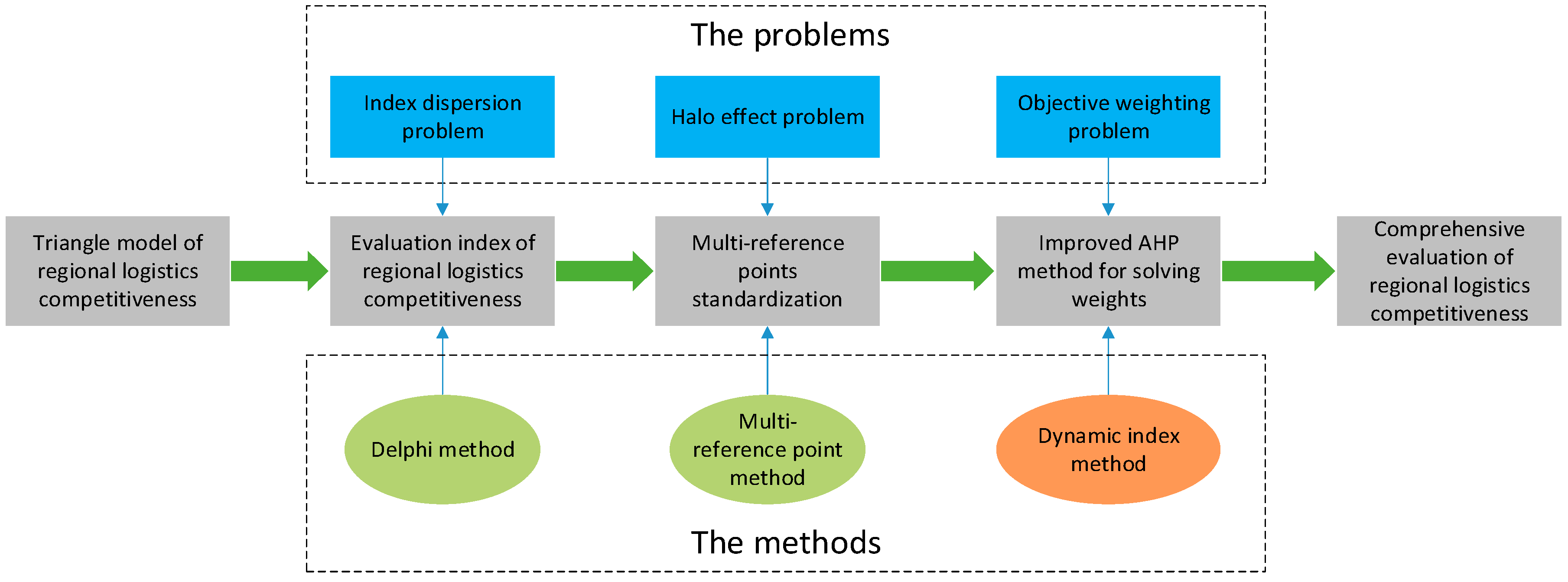
In view of the above reasons, aiming at problems such as the evaluation index system of regional logistics competitiveness being complex and scattered, the normalized distribution of evaluation data being extremely asymmetric and seriously deviating from the normal distribution, and the logic of calculating the index weights by AHP not being accurate, this paper constructs a triangle model of regional logistics competitiveness based on Porter’s diamond model, and it selects closely the related absolute types of indexes from the perspective of the supply chain to build a regional logistics competitiveness evaluation index system. Based on the concept of symmetry theory, a normalization method of segmented mapping with quartiles of various indexes as multi-reference points is proposed by selecting appropriate reference points to standardize the data, thus making the standardized data distribution more reasonable. The dynamic index scale is used to determine the scale of the analytic hierarchy process, and the evaluation matrix is constructed based on the importance level grading table, while the index weights are directly solved without a consistency check, which improves the logical accuracy of the weight calculation of AHP. Then, the index weights are calculated based on an improved analytic hierarchy process. Finally, the comprehensive evaluation value of the logistics competitiveness of each province is weighted, and the evaluation values are sorted and compared. The magnitude of logistics competitiveness can be used as a reference for regional logistics decision-making; this will help provinces and cities recognize the current status of competitiveness in the logistics industry, and this can provide decisions for adjusting the industrial structure, accelerating the construction of logistics infrastructure, and promoting the healthy development of the logistics industry. The method of this paper can be used for multi-criteria decision-making and for a comprehensive evaluation in other fields; the multiple reference points can improve the halo effect (i.e., the index takes a part for the whole) when the index data range is too large, and the dynamic index can improve the analytical quality of the AHP. The research method and framework of this paper are shown in Figure 1.

2. Literature Review

In the process of a comprehensive evaluation, a set of complete evaluation indexes must be determined, and each evaluation index should be given a corresponding weight. Indexes and weights are very important components of a comprehensive evaluation. Weight setting is the key technology of a multi-index comprehensive evaluation, and the rationality and scientificity of the weights directly determine the accuracy of the evaluation results.

2.1. Evaluation Index of Regional Logistics Competitiveness

Regional logistics competitiveness is a combination of multiple factors [2]. The establishment of a relatively perfect evaluation index system is the pre-requisite for grasping the characteristics of regional logistics industry, analyzing the industrial structure, and mastering the level and development trend of industrial competitiveness [11]. Porter (1990) [12] constructed a diamond model to test industrial competitiveness, pointing out that the competitiveness of a country or industry depends on factor conditions (FC), demand conditions (DC), elated and supporting industries (RSD), and firm strategy, structure, and rivalry (FSSR), as well as the interaction between these elements. Li Jianjun et al. (2008) [4] improved Porter’s diamond model and constructed an evaluation model of China’s regional logistics competitiveness from six aspects: the competitiveness of regional logistics enterprises, the factors of regional logistics, the requirements of regional logistics, the regional informatization development level, the regional government’s role, the regional economic development level, and the used factor analysis method; these were used to evaluate the regional logistics competitiveness of 31 provinces in 2008. Xie Ruhe et al. (2008) [11] summarized the evaluation of logistics industry competitiveness into six main indicators: the industrial development environment, industrial organization form and scale, industrial development level, industrial market competitiveness, industrial socialization level, and the overall competitiveness of regional logistics enterprises. C. Jiang and D. Chen (2009) [13] believed that urban logistics infrastructure is an important aspect of urban competitiveness, and they established an evaluation index system for urban logistics capabilities from the aspects of market supply and demand capacity, economic development capacity, and the transportation development level. Gao Xiuli et al. (2010) [3] constructed a regional logistics competitiveness evaluation model from the two dimensions of regional logistics competitiveness and competitiveness potential. Bian Wenliang et al. (2010) [14] constructed a model to describe the competitiveness of the national logistics industry, which consists of three countries, and each country includes three competitive aspects: the competition front-end, the competition fundamentals, and the competition support. Zhao Liqin and Guo Yuexian (2011) [15] divided the evaluation factors of urban logistics competitiveness into three categories: the infrastructure layer, the relevant subject layer, and the service guarantee layer; the general indicators include eight secondary indicators and 32 tertiary indicators. Xue Dongqian (2012) [16] believed that the evaluation of logistics competitiveness of inland central cities should include the level of social and economic development, the logistics demand of related and auxiliary industries, the status of urban logistics infrastructure, the location conditions of the city, the complexity of spatial logistics network, the development level of logistics information technology, etc.; they also established the evaluation index system of seven criteria layers and 29 index layers. Tvaronavi Tchien ė M., razminien ė K (2017) [17] classified cluster performance indicators into three categories—resource, activity, and process—and concluded that the weight of process is 0.7, while the weights of both activity and resource are 0.15. Wang Aihu and tanattarat takurakiat (2018) [18] took the logistics industry of China and Thailand as the research object, and they constructed the evaluation index system of the logistics development level from two dimensions, i.e., logistics competitive strength and logistics competitive potential. Through the analysis of these literature indicators, it can be seen that the evaluation indicators of regional logistics competitiveness are quite different. Porter’s diamond model has advantages in evaluating national competitiveness, but regional logistics has its own unique characteristics, which cannot be directly used to establish the regional logistics competitiveness evaluation system. Through the analysis of an indicator connotation, the logistics factors, logistics demand, and the regional economy are important indicators of logistics competitiveness.

2.2. Method for Determining the Weight of Comprehensive Evaluation Indicators

The methods for determining the weight of comprehensive evaluation indexes include the subjective weighting method, the objective weighting method, and the combination weighting method. The subjective weighting method is a method through which the evaluators or experts obtain the index weight according to their own experience and subjective attention to each index. Subjective weighting methods include the Delphi [19], the analytic hierarchy process (AHP) [20,21], and the analytic network analysis (ANP) [22]. The Delphi method adopts an anonymous way with several rounds of correspondences to seek the opinions of experts so that the evaluation opinions of the expert group can be concentrated, and finally a more consistent index weight is determined. The analytic hierarchy process is to construct a judgment matrix to calculate the weight vector based on the relative importance of the subjective evaluation indexes of the experts. The analytic network analysis method is based on the analytic hierarchy process, taking into account the mutual influence of various factors or adjacent levels, using a “super matrix” to comprehensively analyze each interacting and influencing factor to obtain its mixed weight. The objective weighting method is a method that uses objective information about each index to determine the weight of the index. Objective weighting methods mainly include the mean square difference method [23], the entropy method [24], the gray correlation method [25], and the CRITIC method [26]. The basic idea of the mean square deviation method and the entropy method in determining the objective weight is as follows: If the data sequence of an attribute has more variability, it means that more information is provided, and the more the information is given, the larger the corresponding weight coefficient is. In fact, the gray correlation method to determine the weight of the evaluation index is a quantitative comparison between the weight of each expert’s experience judgment and the maximum value (set) of an expert’s experience judgment; according to the distance, the relevance degree (correlation) of the expert group’s empirical judgment value is calculated. The greater the degree of correlation, the more consistent the expert experience judgment is; moreover, the more important the index is, and the more weight it has. The basic idea of the criteria importance though intercrieria correlation (CRITIC) method is to determine the weight of the indexes based on the contrast strength (standard deviation) and the conflict (correlation coefficient) between evaluation indexes; the greater the conflict and contrast strength between the indexes, the greater the weight of the indexes is. Through a comparative analysis of subjective and objective weighting methods, we can see that both methods have advantages and disadvantages: The subjective empowerment method makes judgments on the importance of the indexes based on the academic level and experience of experts. Although this method is closer to the actual requirements, it cannot objectively and scientifically reflect the data information of the evaluation scheme and is greatly affected by human factors. In some individual cases, the weighting result obtained by applying a subjective weighting method may be significantly different from the actual situation [27]. The objective weighting method takes the amount of information contained in the index as the weight setting standard. It pays attention to the relative difference size of each index value and only determines the index weight based on the relative difference size between the index values; it does not consider the evaluation purpose of the scheme, ignores the requirements of the evaluation purpose for the relative importance of each index, and often deviates from the reality. Due to the different principles of various objective weighting methods, the recognition of the importance of each index is quite different, and the weighting results are also different. In practical applications, the importance of the indexes measured by the objective weighting method may be different from the importance of the subjective cognition, and it cannot accurately reflect the importance of the indexes. For example, the entropy of index A is greater than the entropy of index B; this only indicates that the degree of variation of index A is greater than that of index B, but the role of index A in the comprehensive evaluation is not necessarily greater than that of index B [28]. The combination weighting method combines the subjective and objective weighting methods. It essentially combines the two types of methods, but it does not solve the problems of the two types of methods; the comprehensive weight will change with the coefficient, and it is difficult to reach a consensus on how to determine the weight distribution proportion of the two methods. From the analysis of the methods in these documents, the main components of the regional logistics competitiveness evaluation are the principal component analysis, the factor analysis, the entropy weight method, and the analytic hierarchy process. The factor analysis can only reflect the information of some indicators, and dimensionality reduction will result in the loss of some data information; the entropy weight method only reflects the fluctuation of the internal data of the indicator, and the analytic hierarchy process has the problem of consistency of the judgment matrix. Each method has its own advantages and disadvantages, and so we should make good use of them in practice.

2.3. Evaluation Method of Regional Logistics Competitiveness

Wang Shengyun and Shen Yufang (2007) [29] used the factor analysis method to quantitatively evaluate the regional logistics competitiveness of China in 1997 and 2004; they divided regional logistics competitiveness into five major types, each of which was divided into five levels through the evaluation, and the dynamic types of regional logistics competitiveness were classified and analyzed. Zhou Yarong (2011) [30] used the principal component analysis to conduct a comprehensive evaluation of regional logistics in China and made a simple cluster analysis. Jiang Minglin et al. (2015) [31] and Yang Lei (2015) [32] both used a factor analysis to make an empirical comparative analysis on the level of regional logistics competitiveness in China. Liu Yuanyuan (2016) [33] used the gray correlation method based on combination weighting to evaluate the competitiveness of the logistics industry in 31 provinces and cities across the country, concluding that the development of a regional logistics industry in China is unbalanced and that the regional logistics industry is gradually weakening from east to west. Liu Ruijuan et al. (2017) [34] used the entropy weight technique for order preference by similarity to an ideal solution (TOPSIS) method to dynamically analyze and evaluate the competitiveness of the provincial logistics industry in the new silk road economic belt from 2005 to 2015, and they analyzed the basis of the spatial evolution and spatial agglomeration of logistics competitiveness; the spatial spillover effects of different types of agglomeration areas were quantitatively analyzed. Li Pan and Peng Huiping (2018) [35] used the entropy weight–gray correlation analysis method to study the relationship of regional logistics competitiveness, and they comprehensively analyzed and evaluated the logistics competitiveness of various regions.

3. Comprehensive Evaluation Index System of Regional Logistics Competitiveness

In order to evaluate the competitiveness of regional logistics scientifically and reasonably, it is first necessary to establish a scientific and systematic evaluation index system reflecting the comprehensive competitiveness of regional logistics. The development of regional logistics is inseparable from the support of the regional economy and the upstream and downstream supply chains of the regional logistics industry. The regional logistics competitiveness is not only dependent on the core business areas such as the logistics service capabilities and management capabilities of regional logistics enterprises, but it also depends on the supply ability of an upstream logistics supply chain, such as logistics facilities, equipment, personnel, platforms, etc., as well as the regional logistics environment of a downstream logistics supply chain, such as the effective purchasing power matching of the regional market demand. Therefore, the construction of comprehensive evaluation indexes of regional logistics competitiveness must be selected in accordance with scientific, objective, and relevant principles. At the same time, the availability of statistical data for each evaluation index must be considered. Based on the previous research results, this study combines the characteristics of regional logistics and the opinions of experts. From the perspective of the logistics supply chain, 23 indexes (Table 1) of three categories—namely the resource supply, logistics service, and market demand—are selected for a comprehensive evaluation of regional logistics competitiveness.

3.1. Sample Data Source

Because the annual data statistics of 2018 and 2019 are incomplete, based on the availability and integrity of data, this paper selects 31 provinces in China in 2017 as a research sample to evaluate the competitiveness of regional logistics industries in each province; it should be noted that some annual data of 2018 and 2019 have not been calculated yet. The evaluation index data (data used for calculation) of all provinces and regions in the country are all from the statistical database of the National Bureau of Statistics. Individuals can directly obtain the data of relevant indexes from the official website of the National Bureau of Statistics (http://data.stats.gov.cn). The total amount of social logistics data of each region (data used for reference) is mainly obtained from the 2018 China Logistics Yearbook, and individual data are obtained from China Statistical Yearbook and paper data. All data are objective data to ensure the accuracy and effectiveness of the evaluation index data. Since the current industry classification system of China’s statistical yearbook does not consider the logistics industry as an independent industry, the statistical data of relevant indexes of the logistics industry in this paper are approximately replaced by transportation, warehousing, and postal services.

3.2. Evaluation Index Construction Principles

(1) Scientific principles
From the analysis of the evaluation indexes of most research documents, the evaluation indexes are mainly divided into three categories. One is the absolute quantity index, such as the GDP, which represents the absolute value of the evaluation object. The other is the average quantity index, such as GDP per capita, which represents the unit value of the index. The third is the growth rate index, such as GDP growth rate, which represents the relative value of the index. The nature of the three types of indexes is quite different, and mixed calculations will lead to logical confusion, making the evaluation results unclear. Based on the principle of classification calculation, this article selects absolute indexes for weighting, thereby scientifically reflecting the absolute value of regional logistics competitiveness.
(2) Objectivity principles
In addition to official statistics, most scholars use the expert scoring method to obtain the evaluation scores of government management capabilities in various regions according to the relevant regional logistics planning and the related logistics policies. This method is relatively subjective, and the range of the subjective score is often different from the range of the objective value. In this paper, the official index data such as the statistical yearbook are selected for evaluation, which ensures the objectivity and consistency of the evaluation index data.
(3) Relevance principles
Due to the complexity of the connotation of logistics competitiveness, the construction of evaluation indexes lacks a unified standard. The indexes given by different research papers are quite different. Some indexes have very low correlation with regional logistics competitiveness, which reduces the scientificity and representativeness of the evaluation results. In this paper, the Delphi method is used to select indexes closely related to the evaluation objectives and to build an evaluation index system.

3.3. Construction of an Evaluation Index System

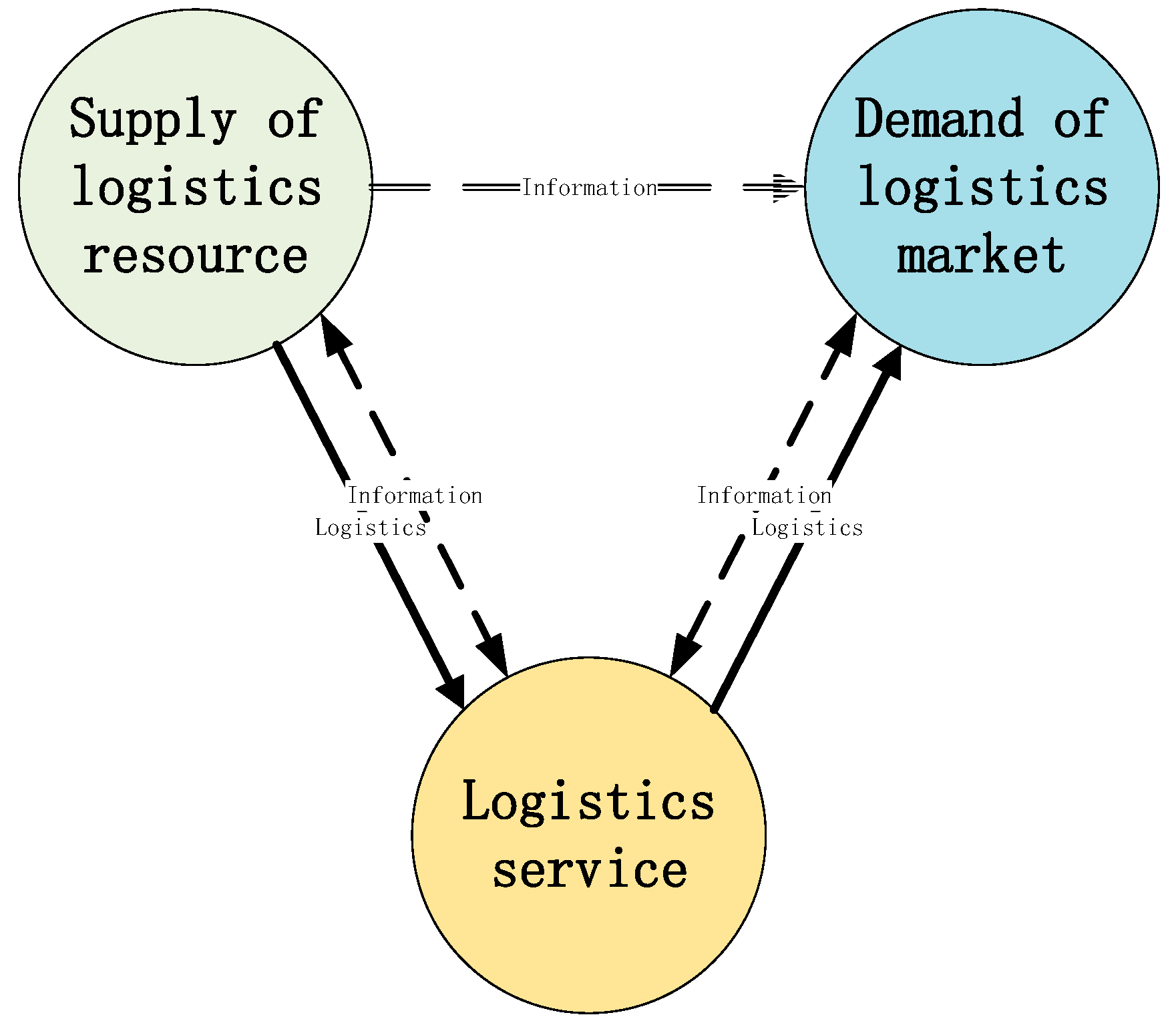
Referring to the previous scholars’ setting of an evaluation index system of regional logistics competitiveness [3,4,6,7,9,10,11,16,18,29,30,31,32,33,34,35,36], according to the description of the indicators, the evaluation indicators are statistically clustered, and the importance of the indicators is decided by the Delphi method. On this foundation, combining the characteristics of regional logistics competitiveness, and considering the scientific, objective, relevant, and available principles of the evaluation indexes, the evaluation indexes are selected from the upstream, middle, and downstream of the logistics industry supply chain based on the perspective of the supply chain. The first is the supply of upstream logistics resources, including logistics units and personnel, logistics assets, logistics channels, etc. The second is the intermediate logistics services, including material flow, logistics value-added services, etc., and the third is the downstream logistics market demand, including production, consumption, circulation, etc. These three aspects interact with each other, and they form the conceptual model of regional logistics competitiveness (Figure 2).
From the eight aspects of the three dimensions of the upstream, middle, and lower downstream, 23 indexes were selected to build a comprehensive evaluation index system of regional logistics competitiveness, as shown in Table 1.

4. Evaluation Method Based on Multiple Reference Points and an Improved Analytic Hierarchy Process

4.1. Problem Description

Let A = {A1,A2,…,Am} denote the set of evaluation objects, and let C be the evaluation index attribute set, where C = {C1,C2,C3,…,Cn}. Let Wj be the attribute index of weight vector Cj; a i , j 0 (I = 1,2,…,m, j = 1,2,3,…,n) is the evaluation matrix, and a i , j 0 represents the index value of the j-th attribute of the i-th evaluation object. This paper studies the ranking of the evaluation objects under multiple indexes, and the difficulties of this type of problem are found in the problem of data processing of the evaluation indexes. Because the maximum value of some indexes is very high, the data of the traditional normalization methods are generally small; moreover, the comprehensive evaluation depends on the scores of several key minority absolute advantage indexes, and the representative mapping of a comprehensive evaluation is not enough. The problem is in determining the weight of the evaluation index. The weight of the evaluation index is an important basis for the evaluation, as the calculation method of the weight directly affects the weight. Because there are many indexes in the subjective weighting method, it is difficult to judge and analyze the weight, and the consistency effect is difficult to guarantee. The objective weighting method is mainly calculated based on the internal data difference of the index, and it has no direct relationship with the actual weight.

4.2. Normalization of Index Values Based on Segment Mapping

Different evaluation indicators usually have different dimensions and orders of magnitude, and the data of the indicators cannot be used for comparison directly. In order to ensure the objectivity and scientificity of the comparison results, it is necessary to standardize the original value of each evaluation object. Through standardized processing, the unit of different attribute indexes is eliminated, and the standardized evaluation index data is additive and comparable. In general, the original data are linearly transformed to map the data to [0,1] or [−1,1]. The methods commonly used for index value standardization are the min-max standardization [37,38], z-score standardization [2], maximum value standardization [39], and the specific gravity method [10]. Taking the dimensionless processing of the sequences x1, x2, …, xn as an example, using the min-max standardization method, the normalized equations of the positive and negative type indexes are expressed as Formulas (1) and (2) [40]:
y i = x i min 1 i n ( x j ) max 1 i n ( x j ) min 1 i n ( x j ) .
y i = max 1 i n ( x j ) x j max 1 i n ( x j ) min 1 i n ( x j ) .
The calculation formula of the z-score standardization method is as follows [2]:
y i = x i x ¯ σ .
In Formula (3), x ¯ and σ are calculated as follows [2]:
x ¯ = 1 n i = 1 n x i .
σ = 1 n 1 i = 1 n ( x i x ¯ ) 2 .
The calculation formula using the maximum value normalization method is as follows [39]:
y i = x i max 1 i n ( x j ) .
The calculation formula of the standardized method using the specific gravity method is as follows [10]:
y i = x i j = 1 n x j .
When the difference between the maximum value and the minimum value of the index value is not too large, the normalized mapping data of the method is not affected by the range, the data distribution is basically uniform and normal. Moreover, the mapping data of different attribute indexes have strong comparability, and the comprehensive evaluation value has more comprehensive representativeness and comprehensiveness. When the range of the evaluation value under an attribute index is too large, the traditional normalization will cause a problem where the comprehensive evaluation result is too greatly affected by some indexes, and it cannot comprehensively reflect the situation of the comprehensive evaluation. Taking the indexes selected for regional logistics competitiveness as an example, there is a large gap between the maximum value of the attribute indexes, the median value, and the minimum value; the ratios of the lowest maximum value and the median value, maximum value, and minimum value of the 23 indexes selected are 2.1 times and 13 times, and the maximum and minimum values of other indexes are tens, hundreds, or even more thousand times. For example, the gap between the maximum value and the minimum value of the express delivery volume, the total import, and export volume, and other indexes in 2017 reached about 1786 and 2473 times, respectively; the normalized median corresponding to about 0.5 is reasonable, which is actually less than 0.05, which is obviously contrary to common sense. In this case, compared with the maximum value, the difference between the smaller evaluation values is almost indistinguishable; even if there is a multiple difference, the score after comparing with the extreme value can be almost ignored. For example, the maximum value of an index is 10,000, and the smaller values (which ranges from 0 to 1000) are in the interval [0,0.1] after normalization. The proportion of the values in this interval may be more, leading to low differentiation, which makes evaluation difficult. The comprehensive score becomes a comparison of whether there is a specialty. If there are no maximum or near-maximum scores, other scores become extremely difficult to determine, making the comprehensive evaluation appear to be a partial phenomenon. This kind of evaluation violates the original intention of the comprehensive evaluation, and it cannot systematically reflect the comprehensive level of the evaluation object. The standardization of the segmented mapping of the index can avoid the problem where the normalized smaller value is extremely weakened due to the existence of the maximum value.
Taking index Cj as an example, we normalize the index value under index Cj to a [0,1] interval value, and we divide the [0,1] interval value into 11 grades, which respectively represent extremely weak [0,0.05), very weak [0.05,0.15), weaker [0.15,0.25), weak [0.25,0.35), lower middle [0.35, 0.45), medium [0.45,0.55), upper middle [0.55,0.65), strong [0.65,0.75), stronger [0.75,0.85), very strong [0.85,0.95), and extremely strong [0.95,1]. The original index values are sorted according to size, and the median of all values is used as the reference point corresponding to the medium evaluation value, which is called the middle reference point; the reference value of the middle reference point is the middle value 0.5 of the scale interval [0,1], and the median of the first half of the evaluation value is taken as the reference point of the upstream and middle evaluation values, which is called the upper and middle reference point. The reference value of the upper and middle reference point is the middle value of the scale interval [0.5,1], which is 0.75 (critical values of strong and stronger). The median of the second half of the evaluation value is taken as the reference point of the middle and downstream evaluation values, which is called the middle and downstream reference point. The reference value of the middle and downstream reference point is the middle value of the scale interval [0,0.5], which is 0.25 (critical values of weaker and weak). According to the setting of the reference points, there are four mapping intervals corresponding to the original evaluation values, and the number of intervals from high to low are [0.75,1], [0.5,0.75], [0.25,0.5], and [0,0.25]. In order to determine the distribution of the actual evaluation values and whether the extreme value of the evaluation value of the index is too large, this paper compared the three dividing points (0.75, 0.5, 0.25) of the mapping interval with the normalized values of the quartiles. The original evaluation value of the index Cj was recorded as a i , j 0 (i = 1,2,3…,m; j = 1,2,3…,n), which has three-quarters quantiles, median, and quarter quantiles recorded as ( a i j 0 )Q3, ( a i j 0 )Q2 and ( a i j 0 )Q1, respectively; correspondingly, the original evaluation data of Cj were divided into four intervals with the quartile as the cut-off point, and the intervals are [( a i , j 0 )Q3,( a i , j 0 )max], [( a i , j 0 )Q2,( a i , j 0 )Q3], [( a i , j 0 )Q1,( a i , j 0 )Q2], [( a i , j 0 )min,( a i , j 0 )Q1] from large to small. In order to reduce the influence range of the maximum value on data normalization and make the normalization ratio better map the difference of the original value, the original value was divided into the first half (the part with large value) and the second half (the part with small value) with the median as the boundary. The first half uses the ratio of three-quarters quantiles of each index to the maximum value, as well as the ratio of the median to the maximum value as the judgment value, and compares it with the reference values of 0.75 and 0.5, respectively. The second half uses the ratio of quarter quantiles of each index to the median value as the judgment value, and compares it with the reference value of 0.5. When the judgment value is greater than or equal to the reference value, it means that the data range is not big, and there is no case that the maximum value is too large, meaning there is no need for interval conversion. When the judgment value is less than the reference value, it means that the data range is too large. In order to make the evaluation value more comparable, it is necessary to perform a rational mapping process on each evaluation value of the original range that is too large to make it more reasonable to map to the corresponding mapping interval.
Assuming that the original interval of the h-th segment of the evaluation target index value under the Cj index is [(( a i , j 0 )min)h,(( a i , j 0 )max)h], the corresponding mapping interval is (( a i , j )min)h,(( a i , j )max)h], the value after the mapping is (aij)h, and the mapping formula of (aij)h is as follows:
( a i j ) h = ( ( a i j ) max ) h ( ( a i j ) min ) h ( ( a i j 0 ) max ) h ( ( a i j 0 ) min ) h ( ( a i j 0 ) h ( ( a i j 0 ) min ) h ) + ( ( a i j ) min ) h ( i = 1 , 2 , , m j = 1 , 2 , , n ) .
According to the normalized value distribution range of the index, the mapping value of the maximum evaluation value under the index Cj is 1, and the mapping value of the minimum evaluation value is converted according to the middle and lower reference points (quarter quantiles). Assuming that the evaluation value of the middle and downstream reference points of the index Cj is (Rj)Q1, the minimum value of Cj is (Rj)min, the reference value of the middle and downstream reference points is (Sj)Q1, and the reference value of the minimum value is recorded as (Sj)min. The formula for (Si)min is as follows:
( S j ) min = ( S j ) Q 1 ( R j ) min ( R j ) Q 1 .
Taking the index Cj as an example, a i j 0 represents the original index value of the j-th attribute of the i-th evaluated object, where the maximum value of the evaluation value under the Cj index is ( a i j 0 )max, the three-quarters quantiles is ( a i j 0 )Q3, the median is ( a i j 0 )Q2, the quarter quantiles is ( a i j 0 )Q1, and the minimum is ( a i j 0 )min. The original evaluation data is arranged from big to small and divided into four intervals according to the quartile: They are [( a i j 0 )Q3,( a i j 0 )max], [( a i j 0 )Q2,( a i j 0 )Q3], [( a i j 0 )Q1,( a i j 0 )Q2], [( a i j 0 )min,( a i j 0 )Q1] in order from big to small. Here, a i j represents the normalized original value of the index of the j-th attribute of the i-th evaluated object, according to the previous normalization processing method of the index value based on the segmentation mapping. The original evaluation value is judged between the partitions, and the normalized processing of the evaluation values is as follows:
(1) For the data in the interval [( a i j 0 )Q3,( a i j 0 )max], when ( a i j 0 )Q3/( a i j 0 )max >= 0.75, no mapping processing is performed. When ( a i j 0 )Q3/( a i j 0 )max < 0.75, the maximum value is found to be too large, and the normalization processing is as follows:
a i j = 0.25 ( a i j 0 ) m a x ( a i j 0 ) Q 3 ( a i j 0 ( a i j 0 ) Q 3 ) + 0.75 .
(2) For the data in the interval [( a i , j 0 )Q2, ( a i , j 0 )Q3], when ( a i , j 0 )Q2/( a i , j 0 )max >= 0.5, no mapping processing is performed; When ( a i , j 0 )Q2/( a i , j 0 )max < 0.5, the maximum value is found to be is too large, and the normalization processing is as follows:
a i j = 0.25 ( a i j 0 ) Q 3 ( a i j 0 ) Q 2 ( a i j 0 ( a i j 0 ) Q 2 ) + 0.50 .
(3) For the data in the interval [( a i , j 0 )Q1, ( a i , j 0 )Q2], when ( a i , j 0 )Q1/( a i , j 0 )Q2 >= 0.5, no mapping processing is performed; When ( a i , j 0 )Q1/( a i , j 0 )Q2 < 0.5, the maximum value is found to be too large, and the normalization processing is as follows:
a i j = 0.25 ( a i j 0 ) Q 2 ( a i j 0 ) Q 1 ( a i j 0 ( a i j 0 ) Q 1 ) + 0.25 .
(4) For the data in the interval [( a i , j 0 )min, ( a i , j 0 )Q1], when ( a i , j 0 )Q1/( a i , j 0 )Q2 >= 0.5, no mapping processing is performed; When ( a i , j 0 )Q1/( a i , j 0 )Q2 < 0.5, the maximum value is found to be too large, and the normalization processing is as follows:
a i j = 0.25 ( a i j ) min ( a i j 0 ) Q 1 ( a i j 0 ) min ( a i j 0 ( a i j 0 ) min ) + ( a i j ) min .
Among them,
( a i j ) min = 0.25 ( a i j 0 ) min ( a i j 0 ) Q 1 .

4.3. Method for Determining Attribute Index Weights Based on an Improved Analytic Hierarchy Process

The analytic hierarchy process (AHP) is a multi-objective decision analysis technology combining both qualitative and quantitative analyses proposed by American operations researcher Saaty [41]. This method takes the form of a proportional scale and makes full use of human experience and judgment. It compares the relative importance of relevant factors at the same level and combines the measures of decision-making objectives from the top to the bottom [35]. Compared with the objective weighting method, the analytic hierarchy process scientifically and reasonably reflects the subjective judgment of the evaluator; this method integrates various qualitative and quantitative factors, and it has certain reliability and validity. Among various studies in different fields, the analytic hierarchy process (AHP) is regarded as the most effective and commonly used multiple-criteria decision-making (MCDM) method [42]. The analytic hierarchy process (AHP) is particularly suitable for the analysis and decision-making of complex systems with multiple objectives, multiple levels, multiple factors, and multiple schemes due to its systemic, flexible, and practical characteristics [43]. However, the scientificity and accuracy of an evaluation using the analytic hierarchy process should be based on reasonable scales and clear logics. The selection of appropriate scales and clear logical relationship judgments are the pre-requisites for the appraisers to make correct judgments.
In the scale setting, the analytic hierarchy process generally uses the numbers 1–9 and their reciprocals as the scale to establish the judgment matrix. According to the scale of 1–9, 1 means equally important, 3 means slightly important, 5 means obviously important, 7 means strongly important, and 9 is extremely important, while 2, 4, 6, and 8 are the median values of neighboring judgments. This scale is simple and clear, but there are some problems, and sometimes the judgment result is far from objective. For example, suppose there are three indexes: A, B, and C. Here, A is slightly more important than B (A/B = 3), and B is slightly more important than C (B/C = 3). The calculation shows that A is more extreme than C in importance (A/C = 9); however, according to the expert’s judgment in the actual research, the importance of A over C will generally be near the position of significant importance (A/C = 5). Moreover, the actual judgment and calculation results are inconsistent, which destroys the consistency of the matrix. In addition to the 1–9 scale, a variety of scales has been proposed, such as the 0 to 2 three-scale method, the −1 to 1 three-scale method, the five-scale system, the 9/9–9/1 scale, the 10/10–18/2 scale, the exponential scale, etc. [44]. Xu Zeshui (2000) [44] compared a variety of scales and found that the 10/10–18/2 scale shows obvious superiority in the accurate weight calculation, and the obtained results are more accurate. The results show that different scale systems are inherently inconsistent.
In terms of logical judgment, the evaluator needs to accurately determine the logical relationship between the indexes. The more evaluation indexes there are, the easier it is for people to compare the indexes, and the more difficult it is to determine the logical relationship between the indexes. When there are many indexes at the same level, the judgments given by the evaluators may even conflict with each other, causing serious inconsistencies in the judgment matrix. However, the consistency of the judgment matrix is a necessary condition for using the analytic hierarchy process. In the application of this method, the inherent defect of the consistency of the judgment matrix has not been overcome; especially when the compared elements are more than 10, the application of this method is even more inaccurate [45].
Aiming at the problem of consistency of judgment matrix constructed by the analytic hierarchy process, this paper proposes an improved analytic hierarchy process method to solve the index weight. The method mainly involves using the chart method to judge the logical relationship between indexes, making the index judgment matrix fully meet the matrix consistency, improving the limitation of the inaccurate method when there are too many elements to be compared, improving the scientificity and logicality of the AHP, using the idea of a dynamic scale decision to establish the scale, and obtaining the subjective weight according to the established index hierarchy model. The specific method is as follows:
(1) Calculate the relationship between indexes through the index importance level classification table
The traditional analytic hierarchy process was used to determine the index weights. First, the evaluation index system was constructed, then the importance of all elements in the next layer compared to the previous layer was compared in pairs, and finally the judgment matrix was constructed. Due to the logical deviation of subjective judgment, the analytic hierarchy process will check the consistency of the judgment matrix. If the test result is within a certain reasonable range, the consistency of the judgment matrix is considered to be is acceptable, and there is no need to adjust the judgment matrix. If the test results are not within a reasonable range, the relationship between the indexes needs to be corrected, and a new judgment matrix is obtained by recalculation. In order to make the comparison between indexes more accurate, all indexes are classified by grade. The grade number does not represent the actual value size, only the importance. The larger the grade value is, the more important the index is. In order to facilitate the conversion, the number of levels of importance and the level of the analytic hierarchy process are the same. Based on the idea of sorting, the indexes were identified in the index importance level classification table by using a check form; after checking, the indexes of different categories were balanced to obtain the final index importance level classification table. Assuming that the index layer to which the subsystem level index B1 belongs has four evaluation indexes of C1, C2, C3, and C4, experts give their importance levels of 9, 5, 3, and 7 respectively. The classification table of the importance of the indexes is given in Table 2.
According to the importance grade judgment in the classification table of importance level of indexes, the relationship between the two indexes was calculated. Taking Ci and Cj as examples, assuming Ci = Pi and Cj = Pj, sgn(PiPj) is a symbolic function, and σ is an arbitrarily small positive real number (make sure that the base of the exponential function is greater than zero). According to the calculation logic of a traditional AHP index comparison, the relationship between Ci and Cj is as follows:
C i C j = ( | P i P j | + σ ) sgn ( P i P j ) .
Taking C1 and C2 for example, C1 = 9, and C2 = 5. According to Formula (13), it is calculated as follows:
C 1 C 2 = ( | P 1 P 2 | + σ ) sgn ( P 1 P 2 ) = ( | 9 5 | + σ ) sgn ( 9 5 ) = 4 C 2 C 1 = ( | P 2 P 1 | + σ ) sgn ( P 2 P 1 ) = ( | 5 9 | + σ ) sgn ( 5 9 ) = 1 4
(2) Establishing scale of exponential function
Using the result of the non-deterministic exponential function y = ux (u > 1, x ≥ 0) and its reciprocal as the scale to establish a judgment matrix, u > 1 makes the exponential function a monotonically increasing function. In order to facilitate identification and comparison, we let the value of the index x be a natural number. When x = 0 and u0 = 1, it means that they are equally important. According to the difference in the importance of the scale and the requirements of the degree of discrimination, the interval of the base number and the index should be determined reasonably. If the maximum value of x is g, then g + 1 is used to represent the scale series. When g = 8, the set of ax corresponds to a scale of 1–9. Assuming that the values of base u are 1.1, 1.2, 1.3, 1.4, and 1.5, the corresponding scale values are shown in Table 3.
(3) Constructing the judgment matrix through scale transformation
Comparing the meaning of the index scales corresponding to the AHP scale classification table in Table 3, the relationship between the two indexes is that C1 is slightly more important than C2. According to the calculation and analysis of the index relationship, if the experts think that the meaning of the index scale description corresponding to the calculation result is far from the original judgment, they can adjust the judgment in Table 3 and then calculate it again until the judgment is basically consistent.
According to the meaning of the exponential function, the calculation result of the relationship between Ci and Cj is equal to the exponent x of the scale function, and the calculation formula is as follows:
x = ( | P i P j | + σ ) sgn ( P i P j ) .
Substituting the result and index scales, the scale conversion formula is as follows:
C i C j = [ u ( | P i P j | + σ ) ] sgn ( P i P j ) .
Taking the evaluation indexes C1, C2, C3, ……, Cn as examples, the judgment matrix of the evaluation indexes is established as follows:
C i j p = [ 1 [ u ( | P 1 P 2 | + σ ) ] sgn ( P 1 P 2 ) [ u ( | P 1 P 3 | + σ ) ] sgn ( P 1 P 3 ) [ u ( | P 1 P n | + σ ) ] sgn ( P 1 P n ) [ u ( | P 2 P 1 | + σ ) ] sgn ( P 2 P 1 ) 1 [ u ( | P 2 P 3 | + σ ) ] sgn ( P 2 P 3 ) [ u ( | P 2 P n | + σ ) ] sgn ( P 2 P n ) [ u ( | P 3 P 1 | + σ ) ] sgn ( P 3 P 1 ) [ u ( | P 3 P 2 | + σ ) ] sgn ( P 3 P 2 ) 1 [ u ( | P 3 P n | + σ ) ] sgn ( P 3 P n ) [ u ( | P n P 1 | + σ ) ] sgn ( P n P 1 ) [ u ( | P n P 2 | + σ ) ] sgn ( P n P 2 ) [ u ( | P n P 3 | + σ ) ] sgn ( P n P 3 ) 1 ]
(4) Calculating the weight of the evaluation index
The weight vector Wj of the evaluation index Cj is calculated by the sum method as follows:
W j = j = 1 n ( u [ ( | P i P j | + σ ) sgn ( P i P j ) ] ) i = 1 n j = 1 n ( u [ ( | P i P j | + σ ) sgn ( P i P j ) ] ) ( I = 1 , 2 , 3 , , n   j = 1 , 2 , 3 , n ) .

4.4. Summary of Methods and Steps

Step 1: Establishing the evaluation scheme characterization
First, a i j 0 represents the original index value of the j-th attribute of the i-th evaluation object, and the evaluation scheme characterization is established as shown in Table 4.
Step 2: Normalizing the index value in sections
If the index is a positive (benefit type) index, the greater the expectation is, the better, and then the index has the maximum polarity and takes the maximum value. If the index is a reverse (cost-type) index, the smaller the expectation is, the better, and then the index has the minimum polarity and takes the minimum value. If the index is a specified value or a medium-sized index, the index has a moderate value polarity, and the specified value or average value is taken. Considering the extreme value of the attribute index, the original data was normalized by using an improved normalization method. Taking the quartile as the dividing point, the original evaluation value was divided into four intervals. According to the ratio and according to the relationship between the ratios of the maximum value of the index (assuming the index is a positive index) and the three-quarters quantiles, the maximum and median, the median and quarter quantiles, and the reference ratio, the data that need to be mapped in sections were transformed to get more scientific and reasonable normalized data.
Step 3: Establishing the scale of the attribute index and calculating the weight of the evaluation index
An improved analytic hierarchy process was used to establish the weights of the evaluation indexes, and the importance difference between the indexes was quantified using the index scale x, in which the index x of u x represents the number of levels of the scale, and the base u represents the cardinal number of the scale. First, the scale series x = p (generally 3, 5, 7, 9 scales are used) of attribute index was determined according to the differentiation, and then the maximum scale ap was determined according to the difference degree of the least important index and the most important index. Next, the scale values corresponding to different levels of scale were obtained by an exponential function. The degree of importance between the indexes from equal importance to extreme importance is represented by 1( u 0), u 1, u 2, u 3,……, u p; conversely, they are represented by their reciprocal. On the basis of the scale value, the importance of indexes was classified with the help of the index importance classification table (Table 3). The evaluation matrix was constructed based on the classification, and the weight vector of each evaluation index was calculated by Formula (13). Since the relationship of indexes is given according to the importance classification table of indexes, the logic of pairwise comparison of indexes is consistent, and the judgment matrix no longer needs to be checked for consistency.
Step 4: Constructing a normalized weighted evaluation matrix Z
The weight of the index Cj is Wj, and the element in the normalized evaluation matrix Z is Zij. The calculation formula of Zij is as follows:
Z i j = a i j W j   ( i = 1 , 2 , 3 , , m   j = 1 , 2 , 3 , , n ) .
Constructing a normalized weighted evaluation matrix is as follows:
Z = [ a 11 W 1 a 12 W 2 a 1 n W n a 21 W 1 a 22 W 2 a 2 n W n a m 1 W 1 a m 2 W 2 a m n W n ]
Step 5: Sorting the evaluation objects based on the comprehensive evaluation value
According to the row vector of the weighted evaluation matrix, the comprehensive evaluation value of each evaluated object was calculated, and the comprehensive evaluation value Zi of the evaluated object Ai was calculated as follows:
Z i = j = 1 n a i j W j ( i = 1 , 2 , 3 , , m   j = 1 , 2 , 3 , , n ) .
The evaluated objects are sorted according to the size of the comprehensive evaluation value.
5. Comprehensive Evaluation and Analysis of Regional Logistics Competitiveness

Regional logistics competitiveness is the value embodiment of regional logistics elements, and the evaluation of regional logistics competitiveness is an important part of regional logistics management. The establishment of a relatively perfect evaluation index system is the pre-condition for grasping the characteristics of the regional logistics industry, analyzing the industrial structure, and grasping the level and development trend of industrial competitiveness. In order to understand the status of regional logistics in various provinces across the country, many scholars have established different evaluation index systems to comprehensively evaluate the competitiveness of regional logistics. From the analysis of the composition of the index system, there are some problems, such as the relationship between the index and regional logistics competitiveness not being close; the absolute indexes, the per capita indexes, and growth indexes being added directly; and there being too many subjective indexes. From the analysis of the index data size, there are many indexes with too large a range, and the existing research rarely pays attention to the influence of range data on evaluation ranking. In the aspect of determining the index weight, the AHP is often used to calculate the index weight; the judgment of logical relationship and the selection of index scale affect the accuracy of the AHP. In view of these problems in the evaluation of regional logistics competitiveness, this paper took the relevant data of 31 provinces in China in 2017 as a research sample, combines the actual situation of regional logistics development, and constructed the evaluation index system of regional logistics competitiveness from the three dimensions of resource supply, logistics service, and market demand. In this paper, the multi-reference point and dynamic index of the improved AHP were used to analyze the regional logistics competitiveness and to evaluate the comprehensive competitiveness of the regional logistics industry in each province, so as to provide a basis for promoting the further development of the regional logistics industry.

5.1. Establishing the Evaluation Scheme Characterization

According to the above research on the comprehensive evaluation index system of regional logistics competitiveness, based on the regional logistics competitiveness evaluation index constructed in Table 1, the evaluation scheme characterization was established. Let Ai (I = 1,2,3,…,31) denote the i-th evaluation target, and let Cj (j = 1,2,3,…,23) denote the j-th evaluation index; a i j 0 (I = 1,2,3,…,31; j = 1,2,3,…,23) represents the original index value of the j-th attribute of the i-th evaluated object and establishes a statistical table of the original index data of the evaluation index (Table A1).

5.2. Normalizing the Index Value

According to the analysis of 23 evaluation indexes, all indexes are positive indexes; the greater the expectations, the better. Because the maximum value of some indexes is too large, if the general normalization method is adopted, the ratio of other data and the extreme value under this index will be seriously unbalanced. The normalized data is concentrated in the left area of the [0,1] interval, which seriously deviates from the normal distribution under the normal condition. Using the three-quarters quantiles and the median of each index as the reference point, in respectively calculating the ratio of each index to the maximum of each index, the ratio is obtained, as shown in Table 5.
According to the normal distribution of the evaluation data, the reasonable ratio of the three-quarters quantiles of the attribute index to the maximum value of the index is about 0.75, and the reasonable ratio of the median to the maximum value is about 0.5. However, the ratios of the three-quarters quantiles and the maximum values in Table 5 are in the interval [0.11,0.61]; all of them are lower than the reference ratio of 0.75. There are 10 indexes whose ratios are lower than 0.33 (the last third); there are 7 indexes below 0.25 (the last quarter), and the ratios of these indexes obviously deviate too much from the reference ratio of 0.75. The ratio of the median to the maximum value of the index is in the range of [0.04,0.48], all of which are lower than the reference ratio of 0.5. There are 15 indexes in which the ratio is lower than 0.25 (the last quarter), 6 indexes in which the ratio is lower than 0.1, and they also significantly deviate from the reference ratio of 0.5. It can be seen that the traditional normalization method using the maximum value as the reference point may cause the normalized values under many indexes to be significantly smaller, and the discrimination is very small. The calculation results will cause the weighted values of multiple indexes to be different. The contribution of the value of the previous index to the comprehensive evaluation value leads to a partial approximation, which causes the evaluation result to be biased and cannot comprehensively reflect the comprehensive competitiveness of the evaluated object. In order to eliminate the problem of excessive deviation of data mapping caused by index extreme values to a certain extent and range, this paper uses multiple reference points to normalize the data. The first half of the data takes the maximum, the three quarters, and median of 31 data sets under each index as reference points, and the second half of the data takes the median, the quarter, and the minimum of 31 data sets under each index as reference points. For reference points, we normalized the original data according to Formulas (13)–(18), and we calculated the standardized data of the original data (Table A2).

5.3. Establishing the Scale of the Attribute Index and Calculating the Weight of the Evaluation Index

According to the calculation results of the index degrees in the scale classification table of the analytic hierarchy process in Table 3, in referring to the number of Grades 1–9 of the Likert scale 9 and in selecting the result of the exponential function y = 1.3x (x = 0,1,2,…,8) (the interval value is closest to the Likert scale 9) and its reciprocal as the scale to establish a judgment matrix, the degree of importance between the indexes from equal importance to extreme importance is 1.0, 1.3, 1.69, 2.20, 2.86, 3.71, 4.83, 6.27, and 8.16 instead, and they are represented by their reciprocal. According to the index importance classification table of Table 3, the experts used the Delphi method to give the index weight level, calculated the relationship between each index according to Formula (8), compared the calculation result with the description of the index relationship, adjusted the index grade when they are inconsistent, iterate to get the original rating judgment matrix (short process), and established the evaluation matrix of the evaluation index according to Formula (10). Because the evaluation indexes of regional logistics competitiveness are divided into a system layer, a subsystem layer, and an index layer, it is necessary to establish an evaluation matrix in layers. Taking the three indexes of the system layer logistics resource supply, the logistics service, and the logistics market demand as examples, the importance level is 7, 9, and 8, and the evaluation matrix of the three indexes is as follows:
A = [ 1 1 1.3 2 1 1.3 1.3 2 1 1.3 1.3 1 1.3 1 ]
Matrix A satisfies the conditions of a uniform matrix a i j a j k = a i k , i, j, k = 1,2,3,…,n, and so the characteristic vector corresponding to the unique non-zero characteristic root of matrix A can be used as the weight vector after normalization; the index weights calculated by the sum vector method are 0.25, 0.42, and 0.33, and the index weights are calculated in turn as shown in Table 6.

5.4. Calculating the Weighted Evaluation Value of Each Index

According to step 4, we constructed the weighted evaluation matrix, calculated the weighted evaluation value according to Formula (19), and obtained the weighted evaluation value of each evaluation index (Table A3).

5.5. Ranking of Evaluation Objects Based on Comprehensive Evaluation Value

According to the row vector of the weighted evaluation matrix in Enclosed Table 3, the comprehensive evaluation value Zi of each evaluated object under the normalization of multiple reference points was calculated by Formula (20). The comprehensive evaluation value (Zi)a, (Zi)b, (Zi)c, and (Zi)d calculated by min-max standardization [37] (Formula (1)), the z-score standardization [2] (Formula (3)), the maximum value standardization [39] (Formula (6)), and the specific gravity method standardization [10] (Formula (7)) are given in Table 7.
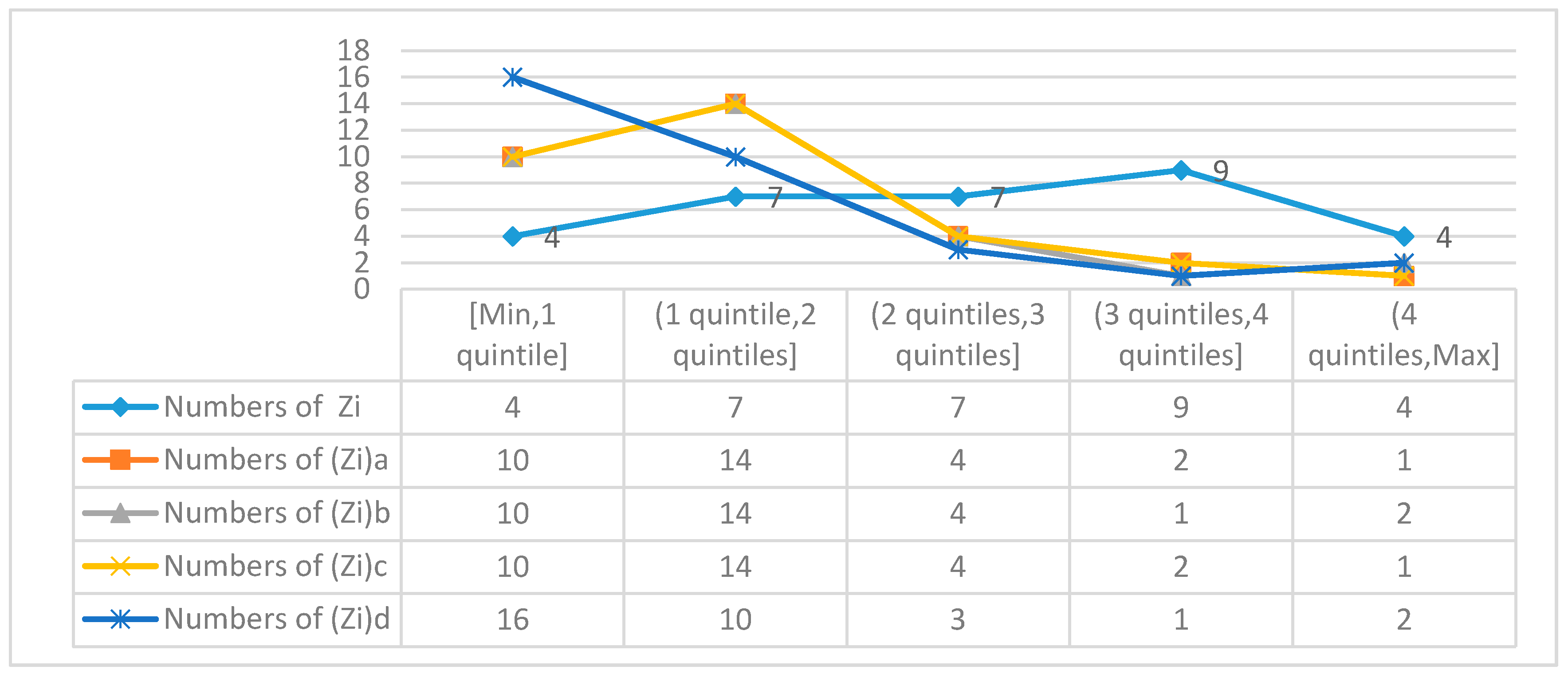
According to the data in Table 7, the number of interval distribution of evaluation values is summarized; the evaluation value is divided into quinquesection intervals (i.e., the interval is divided into 5 equal intervals), and the distribution map of the interval evaluation values is drawn in Figure 3.
From Table 7 and Figure 3, it can be seen that the 31 comprehensive evaluation values calculated by the traditional standard methods such as the min-maximum standardization, Z-score standardization, maximum standardization, and specific gravity method standardization are concentrated on the left side of the quinquesection intervals, and the cumulative number of evaluation values in the two leftmost sections corresponding to the four methods are 24, 24, 24, and 26, accounting for 77.42%, 77.42%, 77.42%, 78.79% respectively of the entire evaluation sample, which deviate from the normal distribution of the evaluation values in general. It can be seen from Figure 1 that the number of comprehensive evaluation values calculated by the method in this paper is more in the middle and less in the two ends, and the number of evaluation values in the quinquesection intervals is basically normal distribution, which can provide a reasonable competitiveness evaluation language through the interval distribution of comprehensive evaluation values, such as five intervals corresponding to strong [0.8,1], relatively strong [0.6,0.8), general [0.4,0.6), relatively weak [0.2,0.4), and weak [0,0.2).
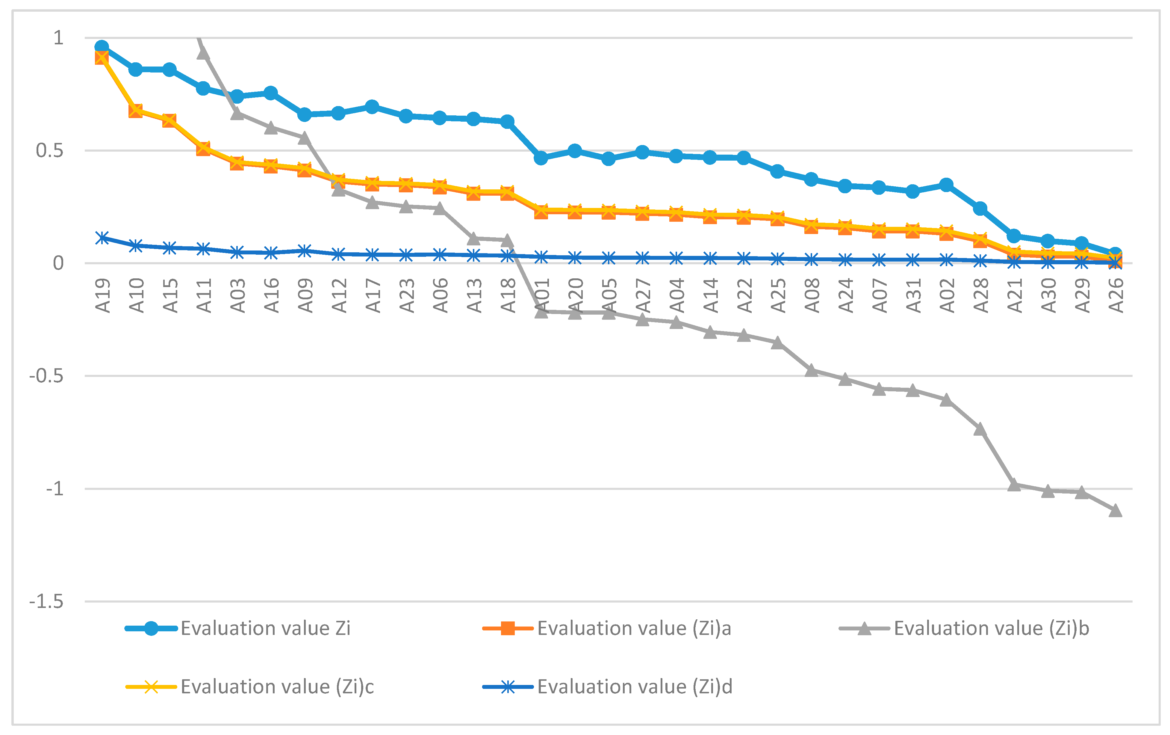
According to the data in Table 7, the evaluated objects are ranked. Since the evaluation index is a positive index, the larger the evaluation value is, the stronger the regional logistics competitiveness of the evaluated object is. The evaluation values Zi are arranged from large to small, and the ranking diagram of regional logistics comprehensive competitiveness under each of the five methods is given in Figure 4.
It can be seen from Figure 4 that the comprehensive evaluation value calculated based on the minimum maximum standardization method and the maximum value standardization method is very close, and the two lines almost coincide, indicating that the range of the original evaluation value of the index is too large. In the data standardization, Formula (1) and Formula (6) original ≈ original − minimum, maximum ≈ maximum − minimum; this leads to the close calculation results of the two methods. From the perspective of the distribution interval of the comprehensive evaluation values, the interval distribution of Zi, (Zi)a, and (Zi)c is more reasonable, and the evaluation value lies in the interval [0,1], which reasonably reflects the gap of the evaluation objects. The interval distribution of (Zi)b and (Zi)d shows two extremes. The evaluation value of (Zi)b is in the interval [−1.1,2.6], and the evaluation value of (Zi)d is in the interval [0,0.11]. When the interval value is magnified 100 times for comparison, the three main intervals are [0,100], [−110,260], [0, 11], which obviously shows that the scoring range in [−110,260] is too large; the scoring range in [0, 11] is too small, and the scoring effect in [0,100] is relatively best. In the case of reasonable range, the comprehensive evaluation value Zi that is calculated based on the standardization method in this paper is relatively uniform in the range, and it is better to avoid the situation in which most of the evaluated objects have low discrimination when the maximum value is too large. Taking the ranking calculated based on the commonly used min-max standardization method and this method as examples, in comparing the ranking differences caused by the two calculation methods, the ranking of the 16 evaluation objects has changed due to the two rankings. Taking A3 and A16 as examples, which are ranked 5 and 6 respectively, Table 6 shows ( Z 16 ) a ( Z 3 ) a , Z 16 Z 3 , which was obtained by directly normalizing the two sets of raw data (Enclosed Table 1) and calculating the comprehensive evaluation value, then obtaining the weighted comprehensive evaluation values of the evaluated objects A3 and A16, which are 0.8673 and 0.8876, respectively; the results show that A16 ranks higher than A3. Similarly, taking A2, A7, A24, and A31, which are ranked 23–26, Table 7 shows ( Z 24 ) a ( Z 7 ) a ( Z 31 ) a ( Z 2 ) a , Z 2 Z 24 Z 7 Z 31 , and the weighted comprehensive evaluation values of the evaluated objects A2, A7, A24, and A31 are 0.7617, 0.6859, 0.7235, and 0.6756, respectively. The ranking is completely consistent with the method in this paper, which illustrates the scientificity and accuracy of the ranking results of this method. In order to further test the sorting effect, the total amount of social logistics was introduced as reference data for judgment. The total amount of social logistics refers to the total value of the goods flowing from the supply place to the receiving place when entering the domestic demand field for the first time. The total amount includes six aspects: the total amount of agricultural products logistics entering the demand field, the total amount of industrial products logistics, the total amount of imported goods logistics, the total amount of transferred goods logistics from other provinces and cities, the total amount of renewable resources logistics, and the total amount of institutions and residents logistics. It can be seen from the content of the index that the total amount of social logistics represents the situation of regional logistics competitiveness to a certain extent. In addition, by comparing the logistics competitiveness rankings of 31 provinces, cities, and autonomous regions in the other studies, a comparison of regional logistics competitiveness rankings is obtained, as given in Table 8.
According to the ranking analysis of 31 provinces, cities, and autonomous regions, the logistics competitiveness in the literature in Table 8, except for a few provinces that are basically the same, most provinces’ rankings are uneven or even very different. For example, the ranking of [33] obviously fluctuates with that of other studies. Because there are no logistics indexes in the current statistical indexes, most evaluations use some indexes of the transportation and postal industries as replacements. With the improvement of statistical indexes, the total social logistics of each province is gradually used as an important statistical index of logistics. Referring to the total social logistics data of some provinces, the ranking of this method is consistent with the total social logistics ranking. Although Guangdong’s total social logistics is lower than Jiangsu’s, many indexes of Guangdong are significantly higher than Jiangsu. In most papers, Guangdong’s logistics competitiveness ranks first, which is consistent with this paper. The top 2–7 and the bottom 27–30 ranks (the total amount of social logistics referenced by the province ranking 31st is missing) of this paper are ranked in the same order as the total social logistics ranking, which reflects the rationality of this index and method. Taking the ranking of the middle cities Beijing as an example, the total amount of social logistics in Beijing in 2017 was 71,105 yuan, which was in the middle and upper reaches. By analyzing the composition of the total amount of social logistics in Beijing in 2017, it was found that the amount of inbound goods logistics in other provinces and cities was 3828.06 billion yuan, accounting for 53.8% of the total amount of social logistics in Beijing, which was much higher than that in the other provinces. In addition, the evaluation indexes of Beijing, namely the amount of highway operation truck ownership (C6), railway operation mileage (C7), highway mileage (C8), inland waterway mileage (C9), freight volume (C13), and freight turnover (C14), are ranked 25, 27, 29, 28, and 29 in 31 provinces respectively. The weight of these indexes is relatively large, and so the logistics competitiveness ranking of Beijing is greatly affected by these indexes, which leads to its ranking in the middle and lower segments. Comparing with the ranking of the other studies, the ranking of this paper is closer to the ranking of total social logistics, which better reflects the level of logistics competitiveness.
According to the comprehensive evaluation value of regional logistics competitiveness, the regional logistics competitiveness is divided into five grades: strong, relatively strong, general medium, relatively weak, and weak; the corresponding evaluation values are located in the intervals of [0.8,1], [0.6,0.8], [0.4,0.6], [0.2,0.4], and [0,0.2), respectively. The regional logistics competitiveness of 31 provinces in China is classified in Table 9.
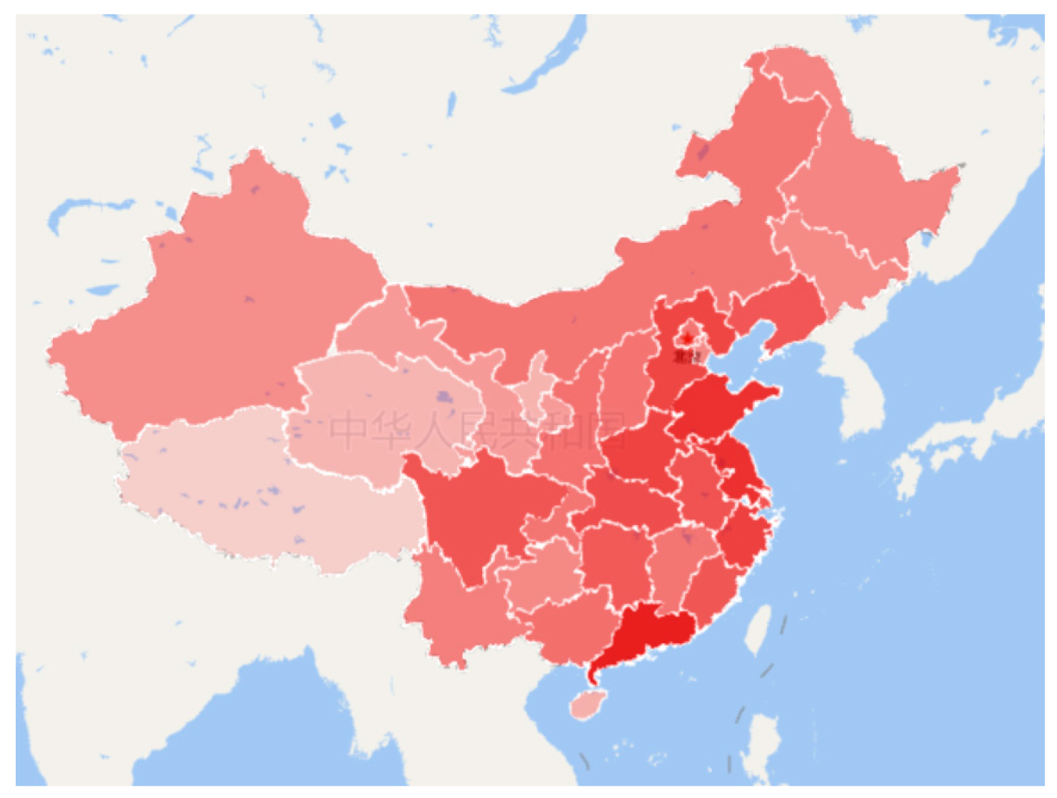
The size of regional logistics competitiveness is indicated in red from a dark to light shade on the map, and the color representation diagram of regional logistics competitiveness is drawn in Figure 5.
According to Table 9 and Figure 5, it can be seen that the regional logistics competitiveness of each province in China is extremely uneven, and the competitiveness obviously decreases from east to west. The three provinces with strong regional logistics competitiveness are all in the southeast coastal areas, and most of the provinces with weak regional logistics competitiveness are in the western inland areas. It can be seen that the competitiveness of regional logistics is closely related to the development level of the local economy. The regional logistics and regional economy complement each other, and so the decision-making of the government departments should consider regional logistics elements and the competitiveness level.

6. Conclusions and Prospection

The evaluation of regional logistics competitiveness is the premise of regional logistics scientific decision-making. In order to improve the scientificity and rationality of the evaluation, the paper addressed the problems of the evaluation index system of regional logistics competitiveness being complex and scattered, the normalized distribution of evaluation data being asymmetric and seriously deviating from the normal distribution, and the logic of calculating the index weights by the AHP not being accurate. To do this, this paper improved and optimized multi-criteria decision-making from three aspects: index selection, data processing, and weight calculation, all of which affect the comprehensive evaluation of regional logistics competitiveness. In the selection of evaluation indexes, in view of the problems of inconsistent types of indexes, subjective data, and the low correlation between indexes and targets, based on the principles of scientificity, objectivity, relevance, and Porter’s diamond model, a triangular model of regional logistics competitiveness was constructed. From the perspective of a supply chain, this paper selected the three dimensions of resource supply, logistics service, and market demand from the perspective of the supply chain to build an evaluation index system. Finally, it determined 23 regional logistics competitiveness evaluation indexes through the Delphi method and expert group decision-making. In terms of index data processing, based on the symmetry theory, the traditional data normalization method was improved. By judging whether the range of evaluation index data is too large, taking the quartile of each index as the reference points, the segment mapping method was adopted for the evaluation data with an extremely large range, which makes the normalized data distribution more reasonable. In terms of weight processing, through improving the index comparison method and scale setting of the AHP, the problem of inconsistent judgment of the logical relationship of indicators is solved, and the dynamic index makes the weight calculation of index more scientific. The evaluation method was applied to the comprehensive evaluation of regional logistics competitiveness of 31 provinces in China, and the evaluation results were obtained and ranked. Comparing and analyzing the evaluation value obtained by this method with the evaluation value calculated by other data standardization methods, it was found that this method can make the standardized data distribution closer to the normal distribution when the data range of evaluation index is too large. Through comparing the ranking of the evaluated objects, the necessity of improving the data normalization was proven, and the scientificity and accuracy of the evaluation was improved. At the same time, the total amount of social logistics was introduced as the reference data for a comparative analysis; it was found that the ranking of regional logistics competitiveness is highly consistent with the total social logistics, and the research shows that the total amount of regional logistics has an important reference value for the competitiveness of regional logistics.
The improved data standardization method can be extended to big data processing in the other fields when the range is too large, which can reduce the influence of the maximum value on the data distribution and improve the comparison discrimination. If the method in this paper is applied to the field of artificial intelligence, the accuracy of machine recognition and judgment can be improved. The triangle model in this paper can be used for a comprehensive evaluation of enterprises and industries, which helps decision makers quickly establish a core evaluation index system from the perspective of the supply chain. The data in this paper uses absolute indexes uniformly to avoid the logical problems caused by the weighted calculation of different attribute data. However, the selection of evaluation indicators in this paper has certain types of limitations. In order to make a more comprehensive evaluation of regional logistics competitiveness, it is also necessary to consider the other types of index data, such as average rate and growth rate, and to study the coupling relationship between different types of indexes. In this paper, only 2017 data were used to evaluate the regional logistics competitiveness. However, regional logistics competitiveness is dynamic. The dynamic evaluation can more comprehensively reflect the development of regional logistics competitiveness, and so the dynamic evaluation of regional logistics competitiveness is a direction to be considered based on panel data. The development of inter-regional logistics industry is not independent because there is a spatial spillover effect or spatial expansion between regions, and there is spatial correlation. The impact of spatial dimension index on regional logistics competitiveness may also be a research innovation, which needs further research. These issues need to be further studied in the future.

Author Contributions

Conceptualization, G.L. and J.Z.; methodology, G.L. and J.Z.; software, G.L.; validation, G.L. and X.L.; formal analysis, G.L.; investigation, G.L.; resources, G.L.; data curation, G.L.; writing—original draft preparation, G.L.; writing—review and editing, G.L., J.Z. and X.L.; visualization, G.L.; supervision, J.Z.; project administration, J.Z.; funding acquisition, J.Z. and X.L. All authors have read and agreed to the published version of the manuscript.

Funding

This research was funded by the National Natural Science Foundation of China (No. 71171112, 71502073, and 71601002) and by the Humanities and Social Sciences Foundation of Ministry of Education of China [No. 16YJC630077].

Conflicts of Interest

The authors declare no conflict of interest.

Appendix A

Table A1. Statistical table of original data of evaluation index.
ProvinceSerial NumberC1C2C3C4C5C6C7C8C9C10C11C12C13C14C15C16C17C18C19C20C21C22C23
BeijingA11491357.6929.5913.331129.1118.710.132.22056561951061208.420110958.42227452.1419.3228014.9411575.416842.1452999.98113.418385.7121618473
TianjinA21937914.544.994.54537.0218.450.111.650.011174862084780.4518002169.5450199.02106.1318549.195729.78424.1727911.62291.72629.4121694799
Hebei A32765724.2736.9816.642135.45144.020.7219.17020328970142497.8822885413381.59119389.3269.0434016.3215907.616055.77211.43101.82441.181535443
Shanxi A41482723.4524.5416.85425.4757.410.5314.290.058930365961052.141895164185.0324359.0772.4215528.426918.18756.377342.32247.5864.320787577
Inner MongoliaA5993821.116.9313.591180.1831.921.2719.940.2428212946051050.022133185146.7611035.3134.3216096.217160.28463.42848.61350.91725.515893414
Liaoning A62010035.5548.232.17602.0176.390.5912.270.0429868471251310.0221613512757.251434.46127.2423409.2413807.213777.313370.33184.82601.5112533837
Jilin A7593816.2542.5818.021211.7432.10.510.390.151835514711603.12499031634.6517569.457.7914944.537855.85799.9120211972.253819792923
Heilongjiang A89726279.858.911200.5448.260.6216.60.511775325818801.33563981657.6923185.6379.4215902.689099.210122.513012.81658.5673.716706937
ShanghaiA91721051.1442.4621.92960.2821.230.051.330.21189648163741344.549685024998.71311503.7711.8730632.9911830.317550.97879037437.315342.3447349338
Jiangsu A106356748.1381.8763.072890.9980.850.2815.852.44539417151903097.672205329057.6359627.8880.9385869.7631737.443020.7543334.111200.86576.6636491742
Zhejiang A113198831.7846.0831.52967.4634.450.2612.010.98758228264871938.1724250410106.23793231.11728.4151768.2624308.525478.9548203.28398.96831.3383972917
Anhui A122345324.2124.117.611667.866.170.4320.330.5618519110652875.3840342611429.7786332.31247.982701811192.613498.8673874104.53299.550986811
Fujian A131912823.9222.2317.62808.8824.220.3210.80.3245671693081889.691322276779.76166110.7392.8632182.091301313150.91227845772.92872.8153077460
Jiangxi A141779820.5525.3111.94734.633.040.4316.230.569025410238866.31544374217.3443754.46129.6520006.317448.110223.223075.31784.8287136920040
Shandong A155275247.6963.1520.423955106.690.5727.060.11452268149363268.013270069719.46151474.6392.8872634.153364935185.9124025.28918.813893316287087
Henan A161897945.1722.7416.932498.5198.180.5426.780.14425176121502162.852301148228.7107377.6332.7144552.8319666.823129.6210126.85157.34407.481368935
Hubei A172555135.3746.7219.992939.8834.340.4226.950.84199008142221420.011881076344.76101277.9265.7435478.0917394.117171.7711901.25897.84411.346200729
Hunan A181348223.4517.4910.82104.3529.250.4723.971.1517070698101496.012255514300.7459181.6192.6433902.9614854.918075.985491.74965.32682.730007933
Guangdong A194966283.3367.5458.553759.667.830.4221.961.212009200242343580.9439238127919.7910134682526.2989705.2338200.145128.9569501.412934.423191.51113658915
GuangxiA201251419.0224.3316.482005.6350.460.5212.330.572639947631955.71746424613.3231750.2988.0418523.26781310505.445501.11929.697152599526
HainanA2120707.078.337.44486.036.30.13.070.03865081714248.9421351864.265915.77194462.541618.82781.821765.9587.5563.913650343
ChongqingA221113427.0123.5319.741954.829.520.2214.790.441365936583939.461155363374.3432874.999.9519424.738067.79290.68143.43534.53572.256569753
Sichuan A231376038.9117.1510.394492.6255.090.48331.08291551189621595.81729222696.17110795.9269.2636980.2217480.519365.698211.55491.33687.866617526
Guizhou A24769812.1710.074.132334.3118.540.3319.440.3714848480471070.22962421656.4815781.953.2313540.8341547506.423808.32092.81434.38120551
Yunnan A251104617.8613.058.373741.7160.350.3724.250.42909667970366.591292981824.9622775.7666.2416376.346423.110506.056853.22472.51329.421386788
TibetA263510.891.211.07581.725.710.088.93064694107334.082203136.3567.513.441310.92523.31045.14108.714077.6610145
Shaanxi A271072327.9614.1312.741891.1639.140.517.440.111693028466832.621630793760.6445750.65116.3121898.818236.49675.259129.23726.91213.740556810
Gansu A28391613.37.322.96956.6430.510.4714.230.091880544863293.5662042439.667201.6826.747459.93426.65148.333525.2913.1412.65000606
Qinghai A2919524.694.344.01730.467.950.238.090.0786279970103.6917923519.461449.716.012624.838391815.421012.1233133450252
NingxiaA3023203.7532.12330.089.60.143.460.01564891319199.3138187753.723721.4715.323443.56930.42113.161210.4330249.54329191
XinjiangA31746216.698.798.291978.531.940.5918.5302083493767668.15843952176.359042.3532.5210881.963044.67272.17376.11140.159730387470
Table A2. Evaluation value after normalization of original data.
C1C2C3C4C5C6C7C8C9C10C11C12C13C14C15C16C17C18C19C20C21C22C23
A10.55 0.87 0.60 0.49 0.32 0.28 0.15 0.07 0.00 0.79 0.33 0.58 0.08 0.14 0.78 0.76 0.64 0.62 0.73 0.88 0.83 0.94 0.75
A20.73 0.30 0.13 0.17 0.16 0.28 0.13 0.05 0.06 0.31 0.14 0.37 0.21 0.29 0.52 0.46 0.46 0.35 0.40 0.79 0.37 0.50 0.75
A30.80 0.51 0.71 0.64 0.58 1.00 0.82 0.69 0.00 0.53 0.46 0.87 0.76 0.81 0.75 0.71 0.75 0.76 0.70 0.49 0.50 0.48 0.62
A40.54 0.49 0.53 0.65 0.13 0.74 0.75 0.45 0.26 0.24 0.43 0.50 0.64 0.50 0.32 0.32 0.39 0.42 0.42 0.50 0.36 0.26 0.27
A50.36 0.44 0.39 0.50 0.33 0.48 1.00 0.74 0.52 0.72 0.30 0.50 0.73 0.55 0.17 0.15 0.40 0.43 0.40 0.22 0.22 0.38 0.22
A60.75 0.75 0.80 0.83 0.18 0.80 0.77 0.39 0.22 0.75 0.47 0.63 0.74 0.80 0.52 0.51 0.56 0.69 0.62 0.64 0.51 0.50 0.73
A70.22 0.34 0.77 0.71 0.34 0.49 0.68 0.33 0.41 0.48 0.31 0.29 0.20 0.23 0.26 0.26 0.37 0.48 0.28 0.15 0.32 0.17 0.26
A80.35 0.57 0.25 0.33 0.33 0.65 0.78 0.54 0.71 0.47 0.38 0.38 0.23 0.24 0.31 0.35 0.40 0.53 0.48 0.23 0.27 0.22 0.23
A90.64 0.83 0.77 0.77 0.28 0.32 0.06 0.04 0.50 0.50 0.83 0.65 0.35 0.96 0.80 0.80 0.69 0.63 0.75 1.00 0.81 0.90 0.83
A101.00 0.82 1.00 1.00 0.78 0.81 0.33 0.50 1.00 0.79 0.81 0.94 0.75 0.76 0.82 0.82 0.98 0.93 0.98 0.84 0.94 0.78 0.88
A110.82 0.67 0.79 0.82 0.79 0.51 0.30 0.38 0.81 0.82 1.00 0.80 0.78 0.77 0.94 0.91 0.83 0.85 0.82 0.86 0.84 0.79 0.82
A120.77 0.51 0.52 0.69 0.45 0.77 0.50 0.75 0.75 0.49 0.70 0.42 1.00 0.79 0.65 0.68 0.63 0.60 0.61 0.50 0.60 0.62 0.52
A130.72 0.50 0.49 0.69 0.77 0.37 0.37 0.34 0.58 0.77 0.61 0.79 0.44 0.65 0.76 0.76 0.72 0.67 0.60 0.77 0.75 0.55 0.76
A140.67 0.43 0.54 0.44 0.22 0.50 0.50 0.52 0.75 0.24 0.67 0.41 0.50 0.50 0.48 0.52 0.50 0.45 0.49 0.23 0.29 0.55 0.42
A150.94 0.81 0.89 0.76 0.93 0.89 0.77 0.88 0.35 0.77 0.81 0.96 0.90 0.76 0.76 0.76 0.92 0.95 0.91 0.77 0.86 0.88 0.80
A160.72 0.80 0.50 0.66 0.70 0.87 0.76 0.88 0.39 0.77 0.76 0.83 0.77 0.73 0.72 0.75 0.80 0.80 0.80 0.56 0.70 0.75 0.62
A170.78 0.75 0.79 0.76 0.79 0.51 0.49 0.88 0.79 0.52 0.80 0.69 0.63 0.62 0.70 0.70 0.76 0.77 0.74 0.61 0.76 0.75 0.50
A180.49 0.49 0.40 0.40 0.57 0.44 0.61 0.82 0.83 0.45 0.64 0.72 0.76 0.51 0.55 0.60 0.75 0.73 0.76 0.38 0.68 0.51 0.36
A190.92 1.00 0.92 0.97 0.90 0.78 0.49 0.79 0.84 1.00 0.96 1.00 0.99 1.00 1.00 1.00 1.00 1.00 1.00 0.93 1.00 1.00 1.00
A200.45 0.40 0.52 0.64 0.54 0.67 0.74 0.39 0.75 0.68 0.50 0.46 0.58 0.52 0.38 0.38 0.46 0.47 0.50 0.38 0.31 0.28 0.52
A210.08 0.15 0.21 0.27 0.14 0.10 0.12 0.10 0.17 0.23 0.11 0.12 0.09 0.12 0.09 0.09 0.11 0.10 0.13 0.13 0.09 0.18 0.19
A220.40 0.57 0.51 0.75 0.52 0.45 0.26 0.47 0.66 0.36 0.43 0.45 0.40 0.42 0.39 0.43 0.49 0.49 0.44 0.52 0.54 0.67 0.54
A230.50 0.77 0.39 0.38 1.00 0.71 0.63 1.00 0.82 0.74 0.88 0.76 0.57 0.35 0.73 0.71 0.76 0.77 0.77 0.52 0.74 0.69 0.57
A240.28 0.25 0.25 0.15 0.65 0.28 0.38 0.71 0.61 0.39 0.53 0.51 0.34 0.24 0.24 0.24 0.34 0.25 0.36 0.28 0.34 0.34 0.11
A250.40 0.37 0.31 0.31 0.90 0.75 0.43 0.83 0.64 0.74 0.52 0.17 0.43 0.26 0.30 0.29 0.41 0.39 0.50 0.47 0.40 0.33 0.28
A260.01 0.02 0.03 0.04 0.17 0.09 0.09 0.28 0.00 0.17 0.07 0.02 0.01 0.02 0.01 0.02 0.03 0.03 0.05 0.01 0.02 0.03 0.01
A270.39 0.59 0.33 0.47 0.50 0.56 0.68 0.59 0.35 0.45 0.56 0.40 0.53 0.46 0.50 0.50 0.53 0.50 0.46 0.54 0.56 0.31 0.45
A280.14 0.28 0.18 0.11 0.28 0.46 0.61 0.45 0.32 0.50 0.32 0.14 0.26 0.32 0.11 0.12 0.19 0.21 0.25 0.26 0.15 0.13 0.07
A290.07 0.10 0.11 0.15 0.22 0.12 0.27 0.26 0.29 0.23 0.06 0.05 0.07 0.07 0.02 0.03 0.07 0.05 0.09 0.08 0.04 0.04 0.01
A300.08 0.08 0.08 0.08 0.10 0.15 0.16 0.11 0.06 0.15 0.09 0.09 0.16 0.11 0.06 0.07 0.09 0.06 0.10 0.09 0.05 0.08 0.06
A310.27 0.35 0.22 0.31 0.53 0.48 0.77 0.66 0.00 0.54 0.25 0.32 0.31 0.29 0.14 0.15 0.27 0.18 0.35 0.50 0.18 0.19 0.36
Table A3. Weighted evaluation value of evaluation index.
C1C2C3C4C5C6C7C8C9C10C11C12C13C14C15C16C17C18C19C20C21C22C23
A10.0099 0.0094 0.0141 0.0190 0.0089 0.0176 0.0022 0.0023 0.0000 0.0033 0.0014 0.0633 0.0074 0.0205 0.0243 0.0308 0.1104 0.0181 0.0365 0.0305 0.0291 0.0052 0.0030
A20.0132 0.0033 0.0029 0.0065 0.0044 0.0173 0.0019 0.0017 0.0008 0.0013 0.0006 0.0406 0.0190 0.0438 0.0160 0.0185 0.0796 0.0102 0.0200 0.0274 0.0129 0.0028 0.0030
A30.0143 0.0055 0.0166 0.0249 0.0162 0.0621 0.0120 0.0223 0.0000 0.0022 0.0019 0.0947 0.0689 0.1211 0.0233 0.0286 0.1287 0.0221 0.0350 0.0171 0.0174 0.0027 0.0025
A40.0098 0.0053 0.0123 0.0253 0.0035 0.0457 0.0110 0.0145 0.0038 0.0010 0.0018 0.0547 0.0574 0.0746 0.0098 0.0129 0.0666 0.0123 0.0208 0.0174 0.0126 0.0015 0.0011
A50.0065 0.0048 0.0090 0.0194 0.0092 0.0300 0.0147 0.0238 0.0077 0.0030 0.0013 0.0546 0.0658 0.0826 0.0051 0.0062 0.0690 0.0127 0.0201 0.0075 0.0076 0.0021 0.0009
A60.0135 0.0081 0.0187 0.0319 0.0050 0.0498 0.0113 0.0125 0.0033 0.0032 0.0020 0.0689 0.0668 0.1198 0.0162 0.0208 0.0963 0.0204 0.0309 0.0223 0.0177 0.0028 0.0029
A70.0039 0.0037 0.0179 0.0275 0.0094 0.0302 0.0101 0.0106 0.0060 0.0020 0.0013 0.0314 0.0183 0.0350 0.0080 0.0105 0.0641 0.0140 0.0138 0.0053 0.0111 0.0010 0.0010
A80.0064 0.0061 0.0058 0.0127 0.0093 0.0402 0.0115 0.0175 0.0105 0.0020 0.0016 0.0417 0.0207 0.0355 0.0095 0.0141 0.0682 0.0155 0.0240 0.0080 0.0093 0.0012 0.0009
A90.0116 0.0090 0.0179 0.0297 0.0077 0.0200 0.0009 0.0014 0.0074 0.0021 0.0035 0.0708 0.0311 0.1435 0.0250 0.0322 0.1185 0.0183 0.0375 0.0348 0.0283 0.0050 0.0033
A100.0180 0.0088 0.0234 0.0387 0.0218 0.0506 0.0048 0.0161 0.0147 0.0033 0.0034 0.1027 0.0679 0.1127 0.0254 0.0329 0.1686 0.0272 0.0489 0.0293 0.0328 0.0043 0.0035
A110.0148 0.0072 0.0184 0.0318 0.0221 0.0319 0.0044 0.0122 0.0118 0.0034 0.0042 0.0872 0.0705 0.1147 0.0292 0.0368 0.1424 0.0248 0.0411 0.0299 0.0294 0.0044 0.0032
A120.0139 0.0055 0.0122 0.0267 0.0125 0.0479 0.0074 0.0243 0.0110 0.0021 0.0029 0.0455 0.0901 0.1173 0.0201 0.0274 0.1074 0.0177 0.0304 0.0174 0.0209 0.0034 0.0020
A130.0130 0.0054 0.0115 0.0267 0.0215 0.0228 0.0055 0.0110 0.0085 0.0032 0.0026 0.0865 0.0397 0.0963 0.0238 0.0307 0.1232 0.0195 0.0298 0.0267 0.0263 0.0030 0.0030
A140.0120 0.0046 0.0126 0.0170 0.0061 0.0311 0.0074 0.0168 0.0110 0.0010 0.0028 0.0450 0.0451 0.0749 0.0150 0.0209 0.0858 0.0132 0.0243 0.0081 0.0100 0.0030 0.0017
A150.0169 0.0088 0.0208 0.0294 0.0259 0.0553 0.0112 0.0285 0.0051 0.0032 0.0034 0.1050 0.0808 0.1140 0.0236 0.0307 0.1585 0.0278 0.0454 0.0269 0.0301 0.0049 0.0032
A160.0129 0.0086 0.0117 0.0255 0.0195 0.0537 0.0111 0.0283 0.0058 0.0032 0.0032 0.0902 0.0690 0.1084 0.0224 0.0304 0.1369 0.0234 0.0400 0.0197 0.0245 0.0042 0.0025
A170.0141 0.0081 0.0185 0.0293 0.0220 0.0318 0.0072 0.0284 0.0116 0.0022 0.0033 0.0750 0.0569 0.0927 0.0218 0.0284 0.1299 0.0226 0.0371 0.0211 0.0265 0.0042 0.0020
A180.0088 0.0053 0.0093 0.0154 0.0159 0.0275 0.0089 0.0265 0.0122 0.0019 0.0027 0.0792 0.0685 0.0756 0.0170 0.0244 0.1285 0.0214 0.0377 0.0134 0.0238 0.0028 0.0014
A190.0166 0.0108 0.0214 0.0377 0.0251 0.0482 0.0072 0.0253 0.0123 0.0042 0.0040 0.1092 0.0888 0.1492 0.0311 0.0404 0.1716 0.0293 0.0499 0.0326 0.0348 0.0055 0.0040
A200.0082 0.0043 0.0122 0.0246 0.0150 0.0415 0.0108 0.0125 0.0110 0.0028 0.0021 0.0497 0.0522 0.0782 0.0118 0.0155 0.0794 0.0139 0.0249 0.0134 0.0108 0.0015 0.0021
A210.0014 0.0016 0.0049 0.0106 0.0040 0.0059 0.0017 0.0031 0.0025 0.0010 0.0005 0.0129 0.0078 0.0185 0.0028 0.0035 0.0191 0.0029 0.0066 0.0047 0.0033 0.0010 0.0007
A220.0073 0.0061 0.0120 0.0292 0.0145 0.0277 0.0038 0.0150 0.0098 0.0015 0.0018 0.0489 0.0357 0.0622 0.0121 0.0175 0.0833 0.0144 0.0221 0.0180 0.0189 0.0037 0.0021
A230.0090 0.0083 0.0091 0.0148 0.0279 0.0443 0.0093 0.0322 0.0120 0.0031 0.0037 0.0826 0.0516 0.0519 0.0228 0.0286 0.1310 0.0227 0.0383 0.0181 0.0257 0.0038 0.0023
A240.0050 0.0027 0.0059 0.0059 0.0180 0.0174 0.0056 0.0228 0.0090 0.0016 0.0022 0.0557 0.0310 0.0355 0.0074 0.0097 0.0581 0.0074 0.0178 0.0098 0.0118 0.0019 0.0004
A250.0072 0.0040 0.0073 0.0119 0.0251 0.0468 0.0063 0.0267 0.0093 0.0031 0.0022 0.0191 0.0390 0.0386 0.0094 0.0119 0.0702 0.0114 0.0249 0.0163 0.0139 0.0018 0.0011
A260.0002 0.0002 0.0007 0.0015 0.0048 0.0054 0.0014 0.0091 0.0000 0.0007 0.0003 0.0018 0.0008 0.0029 0.0003 0.0006 0.0056 0.0009 0.0025 0.0003 0.0008 0.0001 0.0000
A270.0070 0.0063 0.0078 0.0181 0.0140 0.0347 0.0101 0.0191 0.0051 0.0019 0.0023 0.0433 0.0481 0.0681 0.0155 0.0202 0.0916 0.0147 0.0230 0.0189 0.0196 0.0017 0.0018
A280.0026 0.0030 0.0043 0.0042 0.0077 0.0287 0.0089 0.0145 0.0047 0.0021 0.0013 0.0153 0.0237 0.0480 0.0034 0.0049 0.0320 0.0061 0.0122 0.0092 0.0051 0.0007 0.0003
A290.0013 0.0011 0.0025 0.0057 0.0060 0.0075 0.0039 0.0082 0.0042 0.0010 0.0003 0.0054 0.0066 0.0111 0.0007 0.0011 0.0113 0.0015 0.0043 0.0027 0.0013 0.0002 0.0000
A300.0015 0.0008 0.0018 0.0030 0.0027 0.0090 0.0024 0.0035 0.0008 0.0006 0.0004 0.0104 0.0140 0.0161 0.0017 0.0028 0.0148 0.0017 0.0050 0.0032 0.0019 0.0004 0.0002
A310.0049 0.0038 0.0052 0.0118 0.0147 0.0300 0.0113 0.0211 0.0000 0.0023 0.0010 0.0347 0.0281 0.0439 0.0042 0.0059 0.0467 0.0054 0.0173 0.0174 0.0064 0.0011 0.0014

References

  1. Oláh, J.; Sadaf, R.; Máté, D.; Popp, J. The influence of the management success factors of logistics service providers on firms’ competitiveness. Pol. J. Manag. Stud. 2018, 17, 175–193. [Google Scholar] [CrossRef]
  2. Shao, J.; Ma, T.; Dong, S.; Meng, X. Evaluation and Analysis: Development Trend of China’s Logistics Industry under Supply Chain Globalization Environments. J. Serv. Sci. Manag. 2009, 2, 71–79. [Google Scholar] [CrossRef] [Green Version]
  3. GAO, X.; WANG, A. Integrated Evaluation System and Empirical Research of the Regional Logistics Competitiveness. Ind. Eng. Manag. 2010, 15, 41–45. [Google Scholar]
  4. Li, J.; Shu, H.; Qing, F. The Improved Diamond Model’s Application in the Evaluation of Regional Logistics Competitiveness. In Proceedings of the 2010 International Conference on Management of e-Commerce and e-Government, Chengdu, China, 23–24 October 2010; pp. 217–222. [Google Scholar]
  5. Wang, S. Study of Core Competence of Logistics Cluster: The Integration and the Extension of Value Chain. Am. J. Ind. Bus. Manag. 2015, 5, 20–26. [Google Scholar] [CrossRef] [Green Version]
  6. Li, Y.; Liu, M.; Guo, L. Evaluation Model Based on Projection Pursuit Method and Empirical Research of Regional Logistics Low Carbon Competitiveness. Areal Res. Dev. 2015, 34, 28–33. [Google Scholar]
  7. Chung, T.W. A Study on Logistics Cluster Competitiveness among Asia Main Countries using the Porter’s Diamond Model. Asian J. Shipp. Logist. 2016, 32, 257–264. [Google Scholar] [CrossRef]
  8. Grondys, K.; Dragolea, L.L. Logistics attractiveness of Poland in relation to logistics centres and global competition. Pol. J. Manag. Stud. 2016, 14, 84–94. [Google Scholar] [CrossRef]
  9. Gao, J.; Li, X.P. Research on Logistics Competitiveness of Yangtze River Delta Ports from the Perspective of Niche. J. Trans. Technol. 2019, 9, 309–324. [Google Scholar] [CrossRef] [Green Version]
  10. Fan, D.X. The Measurement of Competitiveness of Hong Kong International Shipping Center and Its Promotion Strategies. Mod. Econ. 2019, 10, 853–871. [Google Scholar] [CrossRef] [Green Version]
  11. Xie, R.H.; Qiu, Z.Q.; Chen, B. Index System and Its Application for the Competitiveness of Regional Logistics Industry. Ind. Eng. J. 2008, 11, 109–112. [Google Scholar]
  12. Michael, E. Porter. The competitive advantage of nations. Harv. Bus. Rev. 1990, 68, 73–91. [Google Scholar]
  13. Jiang, C.; Chen, D. Research on Urban Logistics Infrastructure: An Empirical Study of China. J. Serv. Sci. Manag. 2009, 2, 80–91. [Google Scholar] [CrossRef] [Green Version]
  14. Bian, W.L.; Ju, S.D.; Geng, Y. Analysis and evaluation of national logistics competitiveness. J. Beijing Jiaotong Univ. (Soc. Sci. Ed.) 2010, 9, 30–36. [Google Scholar]
  15. Liqin, Z.; Yuexian, G. Research on City Logistics Competitiveness Evaluation Method. Areal Res. Dev. 2011, 30, 78–81. [Google Scholar]
  16. Dongqian, X.; Jing, G.; Shuying, D. On the Logistic Competition of Inland Central Cities in China: A Case Study of Xi’ an and Zhengzhou. Areal Res. Dev. 2012, 30, 78–81. [Google Scholar]
  17. Tvaronavičienė, M.; Razminienė, K. Towards Competitive Regional Development Through Clusters: Approaches To Their Performance Evaluation. J. Compet. 2017, 9, 133–147. [Google Scholar] [CrossRef] [Green Version]
  18. Aihu, W.; Takurakiat, T. Thailand Logistics Industry Development Level Evaluation from Perspective of China-Thailand Comparative Analysis. J. South China Univ. Technol. (Soc. Sci. Ed.) 2018, 103, 32–41. [Google Scholar]
  19. Gong, B.; Zhang, X.; Guo, D.; Gui, Y. Fuzzy Evidential Reasoning Approach for LCMS Competitiveness Evaluation under Incomplete Information. Math. Probl. Eng. 2015, 2015, 949232. [Google Scholar] [CrossRef]
  20. Imran, M.; Jian, Z.; Urbański, M.; Nair, S.L.S. Determinants of firm’s export performance in China’s automobile industry. Sustainability (Switzerland) 2018, 10, 4078. [Google Scholar] [CrossRef] [Green Version]
  21. Sepehr, M.; Fatemi, S.M.R.; Danehkar, A.; Mashinchian Moradi, A. Application of Delphi method in site selection of desalination plants. Glob. J. Environ. Sci. Manag. 2017, 3, 89–102. [Google Scholar]
  22. Weng, S.S.; Chen, K.Y.; Li, C.Y. Application of the Analytic Hierarchy Process and Grey Relational Analysis for Vendor Selection of Spare Parts Planning Software. Symmetry 2019, 11, 1182. [Google Scholar] [CrossRef] [Green Version]
  23. Lin, C.T.; Hsu, S.C. Constructing a Travel Risks’ Evaluation Model for Tour Freelancers Based on the ANP Approach. Adv. Oper. Res. 2016, 2016, 13. [Google Scholar] [CrossRef]
  24. LI, W.W.; YI, P.T.; GUO, Y.J. Comparison of Difference Driving Evaluation Methods in Stability and Difference Highlighting. Oper. Res. Manag. Sci. 2015, 24, 216–221. [Google Scholar]
  25. Zheng, Z.Y.; Liu, J.; Li, Y. Research on Comprehensive Evaluation of Marine Industry in the East Sea Research on Comprehensive Evaluation of Marine Industry in the East Sea. East China Econ. Manag. 2019, 33, 97–102. [Google Scholar]
  26. Wang, B.; Wu, Z.Y. Study on the Comprehensive Evaluation Method of the Competitiveness Urban Culture: Industry from the Perspective of Norm Gray Association with Jiangsu as a Sample. Econ. Probl. 2016, 4, 79–83. [Google Scholar]
  27. Diakoulaki, D.; Mavrotas, G.; Papayannakis, L. Determining objective weights in multiple criteria problems: The CRITIC method. Comput. Oper. Res. 1995, 22, 763–770. [Google Scholar] [CrossRef]
  28. Ze-shui, X.U.; Qing-li, D.A. Study on Method of Combination Weighting. Chin. J. Manag. Sci. 2002, 2, 85–88. [Google Scholar]
  29. Guo, Q. Research on the Index Weight of Logistics Integration in Beijing-Tianjin-Hebei Region Based on Cloud Models. J. Yunnan Univ. Financ. Econ. 2018, 194, 96–104. [Google Scholar]
  30. Yu-fang, W.S.Y.S. The Appraisal and Characters of Provincial Level Logistics Competitiveness in China. China Soft Sci. 2007, 10, 104–110. [Google Scholar]
  31. Ya-rong, Z.H.O.U. PCA-based Comprehensive Evaluation of Regional Logistics Development in China. Logist. Technol. 2011, 30, 88–90. [Google Scholar]
  32. Jiang, M.; Shu, H.; Lin, X.W. Evaluation of Logistics Competitiveness for Six Provinces in Central China Based on Diamond Model. Prices Mon. 2015, 4, 43–48. [Google Scholar]
  33. Yang, L. Analysis and Evaluation of the Regional Logistics Competitiveness. Master’s Thesis, Dalian Jiaotong University, Dalian, China, 2015. [Google Scholar]
  34. Liu, Y.Y. The Regional Logistics Industry Competitiveness Evaluation and Development Strategies. Master’s Thesis, Beijing Jiaotong University, Beijing, China, 2016. [Google Scholar]
  35. Liu, R.J.; Wang, J.W.; Huang, Z.B. Research on Spatial Pattern Evolution and Spillover Effect of “The New Silk Road Economic Belt” Logistics Competitiveness Based on ESDA. Stat. Inf. Forum 2017, 32, 106–112. [Google Scholar]
  36. Pan, L.I.; Hui-ping, P.E.N.G. Evaluation of Regional Logistics Industry Competitiveness of Silk Road Economic Belt. J. Univ. Financ. Econ. 2018, 31, 99–103. [Google Scholar]
  37. Jiang, Y.; Zhang, J.; Asante, D.; Yang, Y. Dynamic evaluation of low-carbon competitiveness(LCC) based on improved Technique for Order Preference by similarity to an Ideal Solution (TOPSIS) method: A case study of Chinese steelworks. J. Clean. Prod. 2019, 217, 484–492. [Google Scholar] [CrossRef]
  38. Liu, G.; Zhu, J.; Liu, X. Imputation Method of Random Arbitrary Missing Data Based on Improved Close Degree of Grey Incidence. J. Grey Syst. 2019, 31, 74–97. [Google Scholar]
  39. Li, Z.J.; Chi, G.T.; Xu, Z.D. Measurement Model of Project Risks of Commercial Banks Based on Combination Weighting. Ind. Eng. Eng. Manag. 2013, 6, 499–509. [Google Scholar]
  40. Satty, T.L. The Analytic Hierarchy Process: Planning, Priority Setting; Mcgraw Hill: New York, NY, USA, 1998. [Google Scholar]
  41. Waris, M.; Panigrahi, S.; Mengal, A.; Soomro, M.I.; Mirjat, N.H.; Ullah, M.; Azlan, Z.S.; Khan, A. An Application of Analytic Hierarchy Process (AHP) for Sustainable Procurement of Construction Equipment: Multicriteria-Based Decision Framework for Malaysia. Math. Probl. Eng. 2019, 2019, 20. [Google Scholar] [CrossRef]
  42. Wang, J.L.; Wu, B.; Xu, Y. Improved AHP Method to Optimize the Weight of Water Supply Performance Indexes. Sci. Technol. Manag. Res. 2019, 9, 49–55. [Google Scholar]
  43. Zeshui, X. A Simulation-Based Evaluation of Several Scales in the Analytic Hierarchy Process. Syst. Eng. Theory Pract. 2000, 20, 58–61. [Google Scholar]
  44. Yan, Z. Construction of Evaluation Index System for Transformation of Scientific and Technological Achievements-Based on Improved Analytic Hierarchy Process. Chin. Univ. Sci. Technol. 2016, 9, 10–11. [Google Scholar]
  45. China Federation of logistics and procurement. In China Logistics Yearbook 2018; China Fortune press: Beijing, China, 2018.
  46. Tian, X.; Zhang, M. Research on Spatial Correlations and Influencing Factors of Logistics Industry Development Level. Sustainability 2019, 11, 1356. [Google Scholar] [CrossRef] [Green Version]
Figure 1. The structure of the research content and method.
Symmetry 12 00847 g001
Figure 2. The triangle model of regional logistics competitiveness.
Symmetry 12 00847 g002
Figure 3. Distribution of the number of evaluation values in quinquesection intervals.
Symmetry 12 00847 g003
Figure 4. Regional logistics comprehensive competitiveness ranking chart based on five standardization methods.
Symmetry 12 00847 g004
Figure 5. The color representation of logistics competitiveness.
Symmetry 12 00847 g005
Table 1. Evaluation indexes of regional logistics competitiveness.
System layer (A)Subsystem layer (B)Index layer (C)
Supply of logistics resources (A1)Logistics unit and personnel (B1)Number of legal entities in transportation, warehousing, and postal services (C1) [31]
Number of employed persons in urban units in transportation, storage, postal, and telecommunications (C2) [30,31,32,33,36]
Number of private enterprises and self-employed persons in transportation, storage, and postal (C3) [30,31,32,33,36]
Number of urban private enterprises and self-employed persons in transportation, storage, and postal (C4) [30,31,32,33,36]
Logistics assets (B2)Investment in fixed assets in transportation, storage, and postal (C5) [6,30,32,33]
The number of trucks in road operation (C6) [6,16,32,33]
Logistics channel (B3)Railway operating mileage (C7) [16,18,29,32,36]
Highway mileage (C8) [6,16,18,30,32,36]
Inland waterway mileage (C9) [18,30,32,36]
Total postal length (C10) [6,33]
Total number of postal outlets (C11) [32,33]
Logistics service (A2)Logistics value-added service (B4)Added value of transportation, storage, and postal industry (C12) [3,33]
Logistics volume (B5)Volume of goods transported (C13) [3,16,18,29,32,33,36]
Volume of goods turnover (C14) [3,6,18,29,30,32,33,36]
Volume of express delivery (C15) [32,33]
Total volume of postal business (C16) [6,33]
Demand of logistics market (A3)Production (B6)GDP (C17) [3,6,16,29,30,31,32,33,36]
Consumption (B7)Total volume of retail sales of social consumer goods (C18) [6,16,32,33]
Final consumption (C19) [33]
Production (B8)Total sales volume of wholesale goods (C20) [3,18]
Volume of total retail sales (C21) [3,18]
Volume of e-commerce sales (C22) [32]
Total volume of import and export volume of destination and source (C23) [16,30,32,33]
Table 2. The classification table of importance level of indexes.
IndexesImportance Level
123456789
B1C1
C2
C3
C4
Table 3. Scale classification of AHP.
Scale NumberIndex Scale (ux)Index Scale (1.1x)Index Scale (1.2x)Index Scale (1.3x)Index Scale (1.4x)Index Scale (1.5x)Index Scale Description
1u011111Indexes are equally important
3u21.211.441.691.962.25 i is slightly more important than j
5u41.462.072.863.845.06 i is obviously more important than j
7u61.772.994.837.5311.39 i is strongly more important than j
9u82.144.38.1614.7625.63 i is extremely more important than j
2u11.11.21.31.41.5Intermediate value of adjacent judgment
4u31.331.732.202.743.38
6u51.612.493.715.387.59
8u71.953.586.2710.5417.09
xux1.1x1.2x1.3x1.4x1.5x
Table 4. Raw value of the evaluation index.
Valuated ObjectsIndex C1Index C2Index C3Index Cn
A1 a 11 0 a 12 0 a 13 0 a 1 n 0
A2 a 21 0 a 22 0 a 23 0 a 2 n 0
A3 a 31 0 a 32 0 a 33 0 a 3 n 0
Am a m 1 0 a m 2 0 a m 3 0 a m n 0
Table 5. The ratio of the reference point to the maximum value of each index.
C1C2C3C4C5C6C7C8C9C10C11C12
Three-quarters quantiles/Maximum value of each index0.310.430.490.300.590.410.410.610.230.150.430.43
Median/Maximum value of each index0.220.290.280.220.420.230.340.480.090.090.290.29
C13C14C15C16C17C18C19C20C21C22C23
Three-quarters quantiles/Maximum value of each index0.54 0.31 0.11 0.12 0.38 0.40 0.38 0.21 0.44 0.17 0.11
Median/Maximum value of each index0.38 0.15 0.05 0.05 0.22 0.22 0.23 0.08 0.24 0.11 0.04
Table 6. Evaluation index weighting of regional logistics competitiveness.
Relative Weight of System Layer ARelative Weight of Subsystem Layer BRelative Weight of Index Layer CAbsolute Weight of Index Layer C
Supply of logistics resources (A1)0.25Logistics unit and personnel (B1)0.36Number of legal entities in transportation, warehousing, and postal services (C1)0.20.018
Number of employed persons in urban units in transportation, storage, postal, and telecommunications (C2)0.120.011
Number of private enterprises and self-employed persons in transportation, storage, and postal (C3)0.260.023
Number of urban private enterprises and self-employed persons in transportation, storage, and postal (C4)0.430.039
Logistics assets (B2)0.36Investment in fixed assets in transportation, storage, and postal (C5)0.310.028
The number of trucks in road operation (C6)0.690.062
Logistics channel (B3)0.28Railway operating mileage (C7)0.210.015
Highway mileage (C8)0.460.032
Inland waterway mileage (C9)0.210.015
Total postal length (C10)0.060.004
Total number of postal outlets (C11)0.060.004
Logistics service (A2)0.42Logistics value-added service (B4)0.26Added value of transportation, storage, and postal industry (C12)10.109
Logistics volume (B5)0.74Volume of goods transported (C13)0.290.090
Volume of goods turnover (C14)0.480.149
Volume of express delivery (C15)0.10.031
Total volume of postal business (C16)0.130.040
Logistics market demand (A3)0.33Production (B6)0.52GDP (C17)10.172
Consumption (B7)0.24Total volume of retail sales of social consumer goods (C18)0.370.029
Final consumption (C19)0.630.050
Production (B8)0.24Total sales volume of wholesale goods (C20)0.440.035
Volume of total retail sales (C21) 0.440.035
Volume of e-commerce sales (C22) 0.070.006
Total volume of import and export volume of destination and source (C23)0.050.004
Table 7. Comprehensive evaluation values of evaluated objects calculated by different methods.
Multi-Reference Point MethodMin-Max StandardizationZ-Score StandardizationMaximum Value StandardizationSpecific Gravity Method Standardization
Evaluated Object Evaluation Value ZiEvaluation Value (Zi)aEvaluation Value (Zi)bEvaluation Value (Zi)cEvaluation Value (Zi)d
A010.4670 0.2263 −0.2145 0.2380 0.0286
A020.3477 0.1309 −0.6045 0.1441 0.0165
A030.7402 0.4426 0.6665 0.4496 0.0490
A040.4758 0.2149 −0.2612 0.2262 0.0236
A050.4637 0.2248 −0.2193 0.2357 0.0242
A060.6450 0.3370 0.2442 0.3468 0.0388
A070.3360 0.1415 −0.5573 0.1534 0.0160
A080.3722 0.1615 −0.4738 0.1729 0.0180
A090.6594 0.4120 0.5579 0.4227 0.0553
A100.8600 0.6762 1.6124 0.6807 0.0781
A110.7760 0.5074 0.9354 0.5152 0.0643
A120.6659 0.3620 0.3273 0.3713 0.0403
A130.6402 0.3089 0.1103 0.3188 0.0359
A140.4695 0.2046 −0.3050 0.2161 0.0231
A150.8593 0.6325 1.4071 0.6365 0.0680
A160.7552 0.4300 0.6029 0.4371 0.0467
A170.6945 0.3494 0.2710 0.3580 0.0385
A180.6282 0.3087 0.1030 0.3183 0.0334
A190.9592 0.9118 2.5934 0.9145 0.1134
A200.4987 0.2259 −0.2190 0.2366 0.0251
A210.1209 0.0375 −0.9811 0.0518 0.0055
A220.4676 0.2027 −0.3178 0.2138 0.0227
A230.6530 0.3465 0.2528 0.3539 0.0367
A240.3428 0.1560 −0.5138 0.1675 0.0167
A250.4076 0.1953 −0.3511 0.2050 0.0206
A260.0410 0.0097 −1.0955 0.0241 0.0022
A270.4928 0.2198 −0.2485 0.2305 0.0241
A280.2427 0.0982 −0.7333 0.1109 0.0114
A290.0879 0.0289 −1.0158 0.0430 0.0042
A300.0988 0.0306 −1.0098 0.0450 0.0046
A310.3188 0.1414 −0.5628 0.1530 0.0154
Table 8. Comparison of regional logistics competitiveness rankings.
Serial NumberProvinceTotal Amount of Social Logistics (billion yuan)Ranking in this PaperRanking in [29]Ranking in [30]Ranking in [31]Ranking in [32]Ranking in [33]
A19Guangdong225,800112117
A10Jiangsu279,563233235
A15Shandong 203,565351328
A11Zhejiang 153,800446444
A16Henan 111,395512461013
A03Hebei 96698.961058712
A17Hubei 87,0287119111116
A12Anhui 60089.5881612141714
A09ShanghaiMissing9210581
A23Sichuan 63909.5101379924
A06Liaoning Missing118810611
A13Fujian 67236.211291513129
A18Hunan 98,480131411121419
A20Guangxi59,912.8142120192322
A27Shaanxi 45315.34152218161521
A04Shanxi 27431.1161819202017
A14Jiangxi 55,430172017212518
A22Chongqing32682.9181723232410
A01Beijing71,10519616752
A05Inner Mongolia33247.9202414181329
A25Yunnan Missing212321242126
A08Heilongjiang 29,500(2015) 221513171625
A02TianjinMissing2372515183
A24Guizhou Missing242826262620
A07Jilin 41464.6(2016) 251922222223
A31XinjiangMissing262529252531
A28Gansu 13623.27272727272727
A21Hainan695828262828296
A30Ningxia6071.8292930293015
A29Qinghai 5210.2303029302828
A26TibetMissing313131313130
Data source: The total social logistics data mainly refer to the 2018 China Logistics Yearbook [46] data, and the ranking is based on the evaluation results in [29,30,31,32,33].
Table 9. The classification of regional logistics competitiveness.
Level of CompetitivenessProvince
Strong Guangdong, Jiangsu, Shandong
Relatively strong Zhejiang, Henan, Hebei, Hubei, Anhui, Shanghai, Sichuan, Liaoning, Fujian, Hunan
GeneralGuangxi, Shaanxi, Shanxi, Jiangxi, Chongqing, Beijing, Inner Mongolia, Yunnan
Relatively weakHeilongjiang, Tianjin, Guizhou, Jilin, Xinjiang, Gansu
Weak Hainan, Ningxia, Qinghai, Tibet