Symmetric Fuzzy Stochastic Differential Equations with Generalized Global Lipschitz Condition ^†

Abstract

The paper contains a discussion on solutions to symmetric type of fuzzy stochastic differential equations. The symmetric equations under study have drift and diffusion terms symmetrically on both sides of equations. We claim that such symmetric equations have unique solutions in the case that equations’ coefficients satisfy a certain generalized Lipschitz condition. To show this, we prove that an approximation sequence converges to the solution. Then, a study on stability of solution is given. Some inferences for symmetric set-valued stochastic differential equations end the paper.

1. Introduction

Stochastic differential equation are natural mathematical tools to describe behavior of many dynamic systems evolving in time. One of the main premises that prompts the use of these equations in description of a studied phenomenon is an assumption that the state of the system is affected by randomness or, more generally, certain stochastic noises. For numerous facts from the theory of these equations, we refer to e.g., [1,2,3,4].

However, many times in the modeling of physical phenomena there is a kind of uncertainty whose nature is different than in the case of randomness. This kind of uncertainty occurs when, for example measurement is not precise and expressed in linguistic terms such as “low pressure”, “high temperature”, and “about 10%”, when opinions of experts are vague, and knowledge of system’s parameters is imperfect. Such the uncertainty is well modeled by application of fuzzy sets (cf. [5,6,7]).

The coexistence of stochastic and fuzzy uncertainties motivates formulating models containing them both. Some successful results of combining randomness and fuzziness have been achieved in, e.g., petroleum contamination [8], optimal tracking design [9], neural networks [10,11], civil engineering and mechanics [12], Petri nets [13], optimization [14], ballast water management [15], option pricing [16], and fuzzy stochastic differential equations [17,18,19,20,21].

The last topic is the subject of this article’s research. In [17,18,19], we considered such equations in their natural integral form, which is a direct reflection of the form of crisp stochastic differential equations, i.e.,

$$x\left(t\right)=x_0\oplus {\int }_0^{t}f(s,x\left(s\right))ds\oplus {\int }_0^{t}g(s,x\left(s\right))dB\left(s\right),t\in [0,T],$$

where f is a fuzzy stochastic mapping, g is a single-valued stochastic mapping, and $x_0$ is a fuzzy random variable. The form of this equation is asymmetric because more components are on the right side of the equation. One could say that this equation is skewed right. In [20,21], the following fuzzy stochastic differential equations

$$x\left(t\right)\oplus (-1)\odot {\int }_0^{t}f(s,x\left(s\right))ds\oplus (-1)\odot {\int }_0^{t}g(s,x\left(s\right))dB\left(s\right)=x_0,t\in [0,T],$$

are studied. This equation is asymmetric as well as the previous one, but now one could say that it is skewed left. If one considers these equations with the structure of single-valued mappings, it is easy to see that they are equivalent and therefore there is no particular reason to consider both equations. However, if the mappings are fuzzy, as in our case, these equations are no longer equivalent. The solution of the first asymmetric equation does not have to be the solution of the second asymmetric equation and vice versa; even the solution (if it exists) of the dual equation does not have to exist on the same interval. Moreover, solutions of both equations generally have the opposite tendency to change fuzziness in their values over time. To be more precise, we mention here that the diameter of the solution’s values cannot decrease as time increases for the first equation, while it cannot increase in the case of the solution to the second equation. This, of course, cannot be observed with single-valued equations.

From a practical point of view, it seems that we cannot limit ourself to just one type of solution, i.e. with nondecreasing fuzziness or nonincreasing fuzziness. Because the fuzziness of solutions may change and return to its previous state, it seems reasonable to consider equations that will ensure that such a requirement is met. Symmetric fuzzy stochastic differential equations

$$\begin{array}{ccc}\hfill x\left(t\right)\oplus (-1)\odot {\int }_0^{t}f(s,x\left(s\right))ds\oplus (-1)\odot {\int }_0^{t}g(s,x\left(s\right))dB\left(s\right)& =& x_0\oplus {\int }_0^t\tilde{f}(s,x\left(s\right))ds\hfill \\ & & \oplus {\int }_0^t\tilde{g}(s,x\left(s\right))d\tilde{B}\left(s\right),t\in [0,T]\hfill \end{array}$$

are such equations. They are also the first fundamental step towards possibility of future research on periodic solutions of fuzzy stochastic differential equations. Neither of the first two equations can have periodic solutions due to the property of monotonicity of fuzziness in successive values. These new symmetric equations do not contain this inconvenience. A symmetric form of these equations is also something special that distinguishes them from classical single-valued equations for which the symmetric form does not make any significant sense. Initial research in the area of symmetric fuzzy stochastic differential equations is made in [22,23] and it needs to be developed. Reference [22] presented a study of this equation with assumption that $f,\tilde{f},g$ and $\tilde{g}$ satisfy a global Lipschitz condition, while, in a conference paper, reference [23] signaled that this condition can be relaxed. The current paper presents in great detail the justification of a theorem from [23] about the existence of a unique solution to the symmetric equation mentioned above with a weaker global condition of the Lipschitz type than in [22]. An analysis of solution stability in the case of small changes in equation parameters is given. In addition, some conclusions for multivalued stochastic equations resulting from the analysis are included.

This paper is organized as follows. Section 2 contains fundamental notations, facts, and properties concerning multivalued random variables, multivalued stochastic processes, fuzzy sets, fuzzy random variables, and fuzzy stochastic Lebesgue–Aumann integral. In Section 3, we present a study on an approximation sequence of fuzzy stochastic processes. With the help of this sequence, existence of the unique solution to symmetric fuzzy stochastic differential equations is proved. In Section 4, we treat about stability of the solution, while Section 5 indicates some inferences from the conducted study to the topic of symmetric multivalued stochastic differential equations. A conclusion in Section 6 summarizes the contribution of the paper.

2. Preliminaries

Almost all listed facts in this section relate to background knowledge and are taken from our work [22]. This is done for the convenience of the reader and to make the paper self-contained.

Let $\mathcal{K}\left({\mathbb{R}}^d\right)$ be the set of all nonempty, compact, and convex subsets of ${\mathbb{R}}^d$. This set can be supplied with the Hausdorff metric $d_H$, which is defined by

$$d_H\left(A,B\right):=max\left\{\underset{a\in A}{sup}\underset{b\in B}{inf}\parallel a-b\parallel ,\underset{b\in B}{sup}\underset{a\in A}{inf}\parallel a-b\parallel \right\},$$

where $\parallel ·\parallel$ denotes a norm in ${\mathbb{R}}^d$. Then, the metric space $(\mathcal{K}\left({\mathbb{R}}^d\right),d_H)$ is complete and separable (see [24]). In addition, the addition and scalar multiplication in $\mathcal{K}\left({\mathbb{R}}^d\right)$ are defined as follows: for $A,B\in \mathcal{K}\left({\mathbb{R}}^d\right)$, $b\in {\mathbb{R}}^d$, $\lambda \in \mathbb{R}$

$$\begin{array}{c}A+B:=\{a+b:a\in A,b\in B\},A+\left\{b\right\}:=\{a+b:a\in A\},\lambda A:=\{\lambda a:a\in A\}.\hfill \end{array}$$

Let $\left(\Omega ,\mathcal{A},P\right)$ be a complete probability space and $\mathcal{M}(\Omega ,\mathcal{A};\mathcal{K}\left({\mathbb{R}}^d\right))$ denote the family of $\mathcal{A}$-measurable multivalued mappings $F:\Omega \to \mathcal{K}\left({\mathbb{R}}^d\right)$ (multivalued random variable) such that

$$\left\{\omega \in \Omega :F\left(\omega \right)\cap O\ne \varnothing \right\}\in \mathcal{A}\mathrm{for} \mathrm{every} \mathrm{open} \mathrm{set}O\subset {\mathbb{R}}^d.$$

A multivalued random variable $F\in \mathcal{M}(\Omega ,\mathcal{A};\mathcal{K}\left({\mathbb{R}}^d\right))$ is called $L^p$-integrally bounded, $p⩾1$, if there exists $h\in L^p\left(\Omega ,\mathcal{A},P;\mathbb{R}\right)$ such that $\parallel a\parallel ⩽h\left(\omega \right)$ for any a and $\omega$ with $a\in F\left(\omega \right)$. It is known (see [25]) that F is $L^p$-integrally bounded iff $\omega \mapsto d_H\left(F\left(\omega \right),\left\{0\right\}\right)$ is in $L^p(\Omega ,\mathcal{A},P;\mathbb{R})$, where $L^p(\Omega ,\mathcal{A},P;\mathbb{R})$ is a space of equivalence classes (with respect to the equality P-a.e.) of $\mathcal{A}$-measurable random variables $h:\Omega \to \mathbb{R}$ such that ${\mathbb{E}\left|h\right|}^p={\int }_{\Omega }{\left|h\right|}^{p}dP<\infty$. Let us denote

$${\mathcal{L}}^p(\Omega ,\mathcal{A},P;\mathcal{K}\left({\mathbb{R}}^d\right)):=\left\{F\in \mathcal{M}(\Omega ,\mathcal{A};\mathcal{K}\left({\mathbb{R}}^d\right)):F\mathrm{is}{L}^p-\mathrm{integrally} \mathrm{bounded}\right\},p⩾1.$$

The multivalued random variables $F,G\in {\mathcal{L}}^p\left(\Omega ,\mathcal{A},P;\mathcal{K}\left({\mathbb{R}}^d\right)\right)$ are considered to be identical, if $F=G$ holds P-a.e.

Let $T>0$, and denote $I:=[0,T]$. Let the system $(\Omega ,\mathcal{A},{\left\{{\mathcal{A}}_t\right\}}_{{}_{t\in I}},P)$ be a complete, filtered probability space with a filtration ${\left\{{\mathcal{A}}_t\right\}}_{{}_{t\in I}}$ satisfying the usual hypotheses, i.e., ${\left\{{\mathcal{A}}_t\right\}}_{{}_{t\in I}}$ is an increasing and right continuous family of sub-$\sigma$-algebras of $\mathcal{A}$, and ${\mathcal{A}}_0$ contains all P-null sets. We call $X:I\times \Omega \to \mathcal{K}\left({\mathbb{R}}^d\right)$ a multivalued stochastic process, if for every $t\in I$ a mapping $X\left(t\right):\Omega \to \mathcal{K}\left({\mathbb{R}}^d\right)$ is a multivalued random variable. We say that a multivalued stochastic process X is $d_H$-continuous, if almost all (with respect to the probability measure P) its paths, i.e., the mappings $X(·,\omega ):I\to \mathcal{K}\left({\mathbb{R}}^d\right)$, are $d_H$-continuous functions. A multivalued stochastic process X is said to be ${\left\{{\mathcal{A}}_t\right\}}_{t\in I}$-adapted, if for every $t\in I$ the multivalued random variable $X\left(t\right):\Omega \to \mathcal{K}\left({\mathbb{R}}^d\right)$ is ${\mathcal{A}}_t$-measurable. It is called measurable, if $X:I\times \Omega \to \mathcal{K}\left({\mathbb{R}}^d\right)$ is a $\mathcal{B}\left(I\right)\otimes \mathcal{A}$-measurable multivalued random variable, where $\mathcal{B}\left(I\right)$ denotes the Borel $\sigma$-algebra of subsets of I. If $X:I\times \Omega \to \mathcal{K}\left({\mathbb{R}}^d\right)$ is ${\left\{{\mathcal{A}}_t\right\}}_{t\in I}$-adapted and measurable, then it is called nonanticipating. Equivalently, X is nonanticipating iff X is measurable with respect to the $\sigma$-algebra $\mathcal{N}$, which is defined as follows

$$\mathcal{N}:=\{A\in \mathcal{B}\left(I\right)\otimes \mathcal{A}:A^t\in {\mathcal{A}}_t\mathrm{for} \mathrm{every} t\in I\},$$

where $A^t=\{\omega :(t,\omega )\in A\}$. A multivalued nonanticipating stochastic process $X:I\times \Omega \to \mathcal{K}\left({\mathbb{R}}^d\right)$ is called ${\mathcal{L}}^p$-integrally bounded, if there exists a measurable stochastic process $h:I\times \Omega \to \mathbb{R}$ such that $\mathbb{E}\left({\int }_I{\left|h\left(s\right)\right|}^{p}ds\right)<\infty$ and $\left|\right|\left|X\right(t,\omega \left)\right|\left|\right|⩽h(t,\omega )$ for a.a. $(t,\omega )\in I\times \Omega$. By ${\mathcal{L}}^p(I\times \Omega ,\mathcal{N};\mathcal{K}\left({\mathbb{R}}^d\right))$, we denote the set of all equivalence classes (with respect to the equality $\gamma \times P$-a.e., $\gamma$ denotes the Lebesgue measure) of nonanticipating and ${\mathcal{L}}^p$-integrally bounded multivalued stochastic processes.

A fuzzy set u in ${\mathbb{R}}^d$ (see [5]) is characterized by its membership function (denoted by u again) $u:{\mathbb{R}}^d\to [0,1]$ and $u\left(x\right)$ (for each $x\in {\mathbb{R}}^d$) is interpreted as the degree of membership of x in the fuzzy set u. As the value $u\left(x\right)$ expresses “degree of membership of x in” or a “degree of satisfying by x a property”, one can work with imprecise information. Obviously, every ordinary set u in ${\mathbb{R}}^d$ is a fuzzy set, since then $u\left(x\right)=1$ if $x\in u$ and $u\left(x\right)=0$ if $x\notin u$.

For a fuzzy set $u:{\mathbb{R}}^d\to [0,1]$ by its $\alpha$-level, $\alpha \in (0,1]$, we mean the set ${\left[u\right]}^{\alpha }:=\{a\in {\mathbb{R}}^d:u\left(a\right)⩾\alpha \}$ and ${\left[u\right]}^0:=\mathrm{cl}\{a\in {\mathbb{R}}^d:u\left(a\right)>0\}$ is called the support of u.

Let $\mathcal{F}\left({\mathbb{R}}^d\right)$ denote the fuzzy sets $u:{\mathbb{R}}^d\to [0,1]$ such that ${\left[u\right]}^{\alpha }\in \mathcal{K}\left({\mathbb{R}}^d\right)$ for every $\alpha \in [0,1]$ and the mapping $\alpha \mapsto {\left[u\right]}^{\alpha }$ is $d_H$-continuous on $[0,1]$. Note that the set ${\mathbb{R}}^d$ can be embedded into $\mathcal{F}\left({\mathbb{R}}^d\right)$ by the embedding $⟨·⟩:{\mathbb{R}}^d\to \mathcal{F}\left({\mathbb{R}}^d\right)$ defined as follows: for $r\in {\mathbb{R}}^d$ we have $⟨r⟩\left(x\right)=1$ if $x=r$, and $⟨r⟩\left(x\right)=0$ if $x\ne r$.

Addition $u\oplus v$ and scalar multiplication $\beta \odot u$ in fuzzy set space $\mathcal{F}\left({\mathbb{R}}^d\right)$ can be defined levelwise

$${[u\oplus v]}^{\alpha }={\left[u\right]}^{\alpha }+{\left[v\right]}^{\alpha },{[\beta \odot u]}^{\alpha }=\beta {\left[u\right]}^{\alpha },$$

where $u,v\in \mathcal{F}\left({\mathbb{R}}^d\right)$, $\beta \in \mathbb{R}$ and $\alpha \in [0,1]$.

Let $u,v\in \mathcal{F}\left({\mathbb{R}}^d\right)$. If there exists $w\in \mathcal{F}\left({\mathbb{R}}^d\right)$ such that $u=v\oplus w$, then we call w the Hukuhara difference of u and v and we denote it by $u\ominus v$. Note that $u\ominus v\ne u\oplus (-1)\odot v$. In addition, $u\ominus v$ may not exist, but if it exists it is unique. For $u,v\in \mathcal{F}\left({\mathbb{R}}^d\right)$ and $r_1,r_2\in {\mathbb{R}}^d$, we have:

(P1)

$(u\oplus ⟨r_1⟩)\ominus ⟨r_2⟩=u\oplus ⟨r_1-r_2⟩$; and

(P2)

the Hukuhara difference $(u\oplus ⟨r_1⟩)\ominus v$ exists iff $u\ominus v$ exists. Moreover, $(u\oplus ⟨r_1⟩)\ominus v=(u\ominus v)\oplus ⟨r_1⟩$.

Define $d_{\infty }:\mathcal{F}\left({\mathbb{R}}^d\right)\times \mathcal{F}\left({\mathbb{R}}^d\right)\to [0,\infty )$ by the expression

$$d_{\infty }(u,v):=\underset{\alpha \in [0,1]}{sup}{d}_H({\left[u\right]}^{\alpha },{\left[v\right]}^{\alpha }).$$

The mapping $d_{\infty }$ is a metric in $\mathcal{F}\left({\mathbb{R}}^d\right)$. It is known that $(\mathcal{F}\left({\mathbb{R}}^d\right),d_{\infty })$ is a complete metric space, but it is not separable and it is not locally compact. For every $u,v,w,z\in \mathcal{F}\left({\mathbb{R}}^d\right)$, $\beta \in \mathbb{R}$ one has (see, e.g., [26])

(P3)

$d_{\infty }(u+w,v+w)=d_{\infty }(u,v)$;

(P4)

$d_{\infty }(u+v,w+z)⩽d_{\infty }(u,w)+d_{\infty }(v,z)$;

(P5)

$d_{\infty }(\beta u,\beta v)=\left|\beta \right|d_{\infty }(u,v)$;

(P6)

$d_{\infty }(u\ominus v,⟨0⟩)=d_{\infty }(u,v)$;

(P7)

$d_{\infty }(u\ominus v,u\ominus w)=d_{\infty }(v,w)$; and

(P8)

$d_{\infty }(u\ominus v,w\ominus z)⩽d_{\infty }(u,w)+d_{\infty }(v,z)$.

A mapping $x:\Omega \to \mathcal{F}\left({\mathbb{R}}^d\right)$ is said to be a fuzzy random variable (see [26]), if ${\left[x\right]}^{\alpha }:\Omega \to \mathcal{K}\left({\mathbb{R}}^d\right)$ is an $\mathcal{A}$-measurable multivalued random variable for all $\alpha \in [0,1]$. It is known from [27] that $x:\Omega \to \mathcal{F}\left({\mathbb{R}}^d\right)$ is the fuzzy random variable iff $x:(\Omega ,\mathcal{A})\to (\mathcal{F}\left({\mathbb{R}}^d\right),{\mathcal{B}}_{d_{\infty }})$ is $\mathcal{A}|{\mathcal{B}}_{d_{\infty }}$-measurable. A fuzzy random variable $x:\Omega \to \mathcal{F}\left({\mathbb{R}}^d\right)$ is said to be $L^p$-integrally bounded, $p⩾1$, if ${\left[x\right]}^0$ belongs to ${\mathcal{L}}^p(\Omega ,\mathcal{A},P;\mathcal{K}\left({\mathbb{R}}^d\right))$. By ${\mathcal{L}}^p(\Omega ,\mathcal{A},P;\mathcal{F}\left({\mathbb{R}}^d\right))$, we denote the set of all $L^p$-integrally bounded fuzzy random variables, where we consider $x,y\in {\mathcal{L}}^p(\Omega ,\mathcal{A},P;\mathcal{F}\left({\mathbb{R}}^d\right))$ as identical if $x=y$ holds P-a.e. In the set ${\mathcal{L}}^2(\Omega ,\mathcal{A},P;\mathcal{F}\left({\mathbb{R}}^d\right))$, one can define a metric $\rho$ by $\rho (x,y):={\left(\mathbb{E}{d}_{\infty }^2(x,y)\right)}^{1/2}$. Then, the metric space $\left({\mathcal{L}}^2(\Omega ,\mathcal{A},P;\mathcal{F}\left({\mathbb{R}}^d\right)),\rho \right)$ is complete (see [28]).

We call $x:I\times \Omega \to \mathcal{F}\left({\mathbb{R}}^d\right)$ a fuzzy stochastic process, if for every $t\in I$ the mapping $x(t,·):\Omega \to \mathcal{F}\left({\mathbb{R}}^d\right)$ is a fuzzy random variable. We say that a fuzzy stochastic process x is $d_{\infty }$-continuous, if almost all (with respect to the probability measure P) its trajectories, i.e., the mappings $x(·,\omega ):I\to \mathcal{F}\left({\mathbb{R}}^d\right)$ are the $d_{\infty }$-continuous functions. A fuzzy stochastic process x is called ${\left\{{\mathcal{A}}_t\right\}}_{t\in I}$-adapted, if for every $\alpha \in [0,1]$ the multifunction ${\left[x\left(t\right)\right]}^{\alpha }:\Omega \to \mathcal{K}\left({\mathbb{R}}^d\right)$ is ${\mathcal{A}}_t$-measurable for all $t\in I$. It is called measurable, if ${\left[x\right]}^{\alpha }:I\times \Omega \to \mathcal{K}\left({\mathbb{R}}^d\right)$ is a $\mathcal{B}\left(I\right)\otimes \mathcal{A}$-measurable multifunction for all $\alpha \in [0,1]$, where $\mathcal{B}\left(I\right)$ denotes the Borel $\sigma$-algebra of subsets of I. If $x:I\times \Omega \to \mathcal{F}\left({\mathbb{R}}^d\right)$ is ${\left\{{\mathcal{A}}_t\right\}}_{t\in I}$-adapted and measurable, then it is called nonanticipating. Equivalently, x is nonanticipating iff for every $\alpha \in [0,1]$ the multivalued random variable ${\left[x\right]}^{\alpha }$ is measurable with respect to the $\sigma$-algebra $\mathcal{N}$. A fuzzy stochastic process x is called $L^p$-integrally bounded ($p⩾1$), if there exists a measurable stochastic process $h:I\times \Omega \to \mathbb{R}$ such that $\mathbb{E}{\int }_I{\left|h\left(t\right)\right|}^{p}dt<\infty$ and $d_{\infty }(x(t,\omega ),⟨0⟩)⩽h(t,\omega )$ for a.a. $(t,\omega )\in I\times \Omega$. By ${\mathcal{L}}^p(I\times \Omega ,\mathcal{N};\mathcal{F}\left({\mathbb{R}}^d\right))$, we denote the set of nonanticipating and $L^p$-integrally bounded fuzzy stochastic processes.

In the whole paper, notation $x\stackrel{P.1}{=}y$ stands for abbreviation of $P\left(x=y\right)=1$, where $x,y$ are some random elements. In addition, we write $x\left(t\right)\stackrel{IP.1}{=}y\left(t\right)$ instead of $P\left(x\left(t\right)=y\left(t\right)\forall t\in I\right)=1$, where $x,y$ are some stochastic processes. Similar notations are used for inequalities.

Let $x\in {\mathcal{L}}^p(I\times \Omega ,\mathcal{N};\mathcal{F}\left({\mathbb{R}}^d\right))$, $p⩾1$. For such the process x, we can define (see, e.g., [17]) the fuzzy stochastic Lebesgue–Aumann integral which is a fuzzy random variable

$$\Omega \ni \omega \mapsto {\int }_{I}x(s,\omega )ds\in \mathcal{F}\left({\mathbb{R}}^d\right).$$

Then, ${\int }_0^{t}x\left(s\right)ds$ (from now on, we do not write the argument $\omega$) is understood as ${\int }_I{\mathbf{1}}_{[0,t]}\left(s\right)x\left(s\right)ds$. For the fuzzy stochastic Lebesgue–Aumann integral, we have the following properties (see [17]).

Lemma 1.

Let $p⩾1$. If $x,y\in {\mathcal{L}}^p(I\times \Omega ,\mathcal{N};\mathcal{F}\left({\mathbb{R}}^d\right))$, then:

(i)

$I\times \Omega \ni (t,\omega )\mapsto {\int }_0^{t}x(s,\omega )ds\in \mathcal{F}\left({\mathbb{R}}^d\right)$ belongs to ${\mathcal{L}}^p(I\times \Omega ,\mathcal{N};\mathcal{F}\left({\mathbb{R}}^d\right))$;

(ii)

the fuzzy process $(t,\omega )\mapsto {\int }_0^{t}x(s,\omega )ds$ is $d_{\infty }$-continuous;

(iii)

$$\underset{u\in [0,t]}{sup}{d}_{\infty }^p\left({\int }_0^{u}x\left(s\right)ds,{\int }_0^{u}y\left(s\right)ds\right)\stackrel{IP.1}{⩽}{t}^{p-1}{\int }_0^t{d}_{\infty }^p\left(x\left(s\right),y\left(s\right)\right)ds;$$

and

(iv)

for every $t\in I$, it holds

$$\mathbb{E}\underset{u\in [0,t]}{sup}{d}_{\infty }^p\left({\int }_0^{u}x\left(s\right)ds,{\int }_0^{u}y\left(s\right)ds\right)⩽t^{p-1}\mathbb{E}{\int }_0^t{d}_{\infty }^p\left(x\left(s\right),y\left(s\right)\right)ds.$$

As we mentioned, e.g., in [17,19], it is not possible to define fuzzy stochastic integral of Itô type such that it is not a crisp random variable. Hence, we consider the diffusion part of the fuzzy stochastic differential equation as the crisp stochastic Itô integral whose values are embedded into $\mathcal{F}\left({\mathbb{R}}^d\right)$.

For convenience of the reader, we give also formulation of the Bihari inequality that is useful in the paper.

Lemma 2.

(Bihari’s inequality, see, e.g., Theorem 1.8.2 in [3]). Let $T>0$ and $c>0$. Let $\xi :{\mathbb{R}}_{+}\to {\mathbb{R}}_{+}$ be a continuous nondecreasing function such that $\xi \left(t\right)>0$ for every $t>0$. Let $u(·)$ be a Borel measurable bounded nonnegative function on $[0,T]$, and let $v(·)$ be a non-negative integrable function on $[0,T]$. If $u\left(t\right)⩽c+{\int }_0^{t}v\left(s\right)\xi \left(u\left(s\right)\right)dsfor everyt\in [0,T],$ then $u\left(t\right)⩽J^{-1}\left(J\left(c\right)+{\int }_0^{t}v\left(s\right)ds\right)$ holds for all such $t\in [0,T]$ that $J\left(c\right)+{\int }_0^{t}v\left(s\right)ds\in \mathrm{Dom}\left(J^{-1}\right)$, where $J\left(r\right)={\int }_1^r\frac{ds}{\xi \left(s\right)}$, $r>0$, and $J^{-1}$ is the inverse function of J. Moreover, if $c=0$ and ${\int }_{0+}\frac{ds}{\xi \left(s\right)}=\infty$, then $u\left(t\right)=0$ for every $t\in [0,T]$.

3. Unique Solutions

The purpose of this paper is to study the symmetric fuzzy stochastic differential equations which in their integral form can be written as follows

$$\begin{array}{c}x\left(t\right)\oplus (-1)\odot {\int }_0^{t}f(s,x\left(s\right))ds\oplus ⟨\sum _{i=1}^m{\int }_0^t(-1)g^i(s,x\left(s\right))d{B}^i\left(s\right)⟩\stackrel{IP.1}{=}{x}_0\oplus {\int }_0^t\tilde{f}(s,x\left(s\right))ds\\ \oplus ⟨\sum _{j=1}^n{\int }_0^t{\tilde{g}}^j(s,x\left(s\right))d{\tilde{B}}^j\left(s\right)⟩,\end{array}$$

where $f,\tilde{f}:I\times \Omega \times \mathcal{F}\left({\mathbb{R}}^d\right)\to \mathcal{F}\left({\mathbb{R}}^d\right)$, $g:I\times \Omega \times \mathcal{F}\left({\mathbb{R}}^d\right)\to {\mathbb{R}}^d\times {\mathbb{R}}^m$, $\tilde{g}:I\times \Omega \times \mathcal{F}\left({\mathbb{R}}^d\right)\to {\mathbb{R}}^d\times {\mathbb{R}}^n$, $x_0:\Omega \to \mathcal{F}\left({\mathbb{R}}^d\right)$ is a fuzzy random variable, and $B^1,B^2,\dots ,B^m,{\tilde{B}}^1,{\tilde{B}}^2,\dots ,{\tilde{B}}^n$ are the independent, one-dimensional ${\left\{{\mathcal{A}}_t\right\}}_{t\in I}$-Brownian motions.

By applying Properties (P1) and (P2), we obtain an equivalent form of the above equation, i.e.,

$$\begin{array}{c}\hfill x\left(t\right)\stackrel{IP.1}{=}\left[x_0\oplus {\int }_0^t\tilde{f}(s,x\left(s\right))ds\right]\ominus \left[(-1)\odot {\int }_0^{t}f(s,x\left(s\right))ds\right)]\oplus ⟨\sum _{k=1}^{\ell }{\int }_0^t{h}^k(s,x\left(s\right))d{W}^k\left(s\right)⟩,\end{array}$$

(1)

where $\ell =m+n$, $h^1,h^2,\dots ,h^{\ell }:I\times \Omega \times \mathcal{F}\left({\mathbb{R}}^d\right)\to {\mathbb{R}}^d$, $h^1\equiv g^1,\dots ,h^m\equiv g^m$, $h^{m+1}\equiv {\tilde{g}}^1,\dots ,h^{m+n}\equiv {\tilde{g}}^n$ and $W^1,W^2,\dots ,W^{\ell }$ are the independent one-dimensional ${\left\{{\mathcal{A}}_t\right\}}_{t\in I}$-Brownian motions, $W^1\equiv B^1,\dots ,W^m\equiv B^m$, $W^{m+1}\equiv {\tilde{B}}^1,\dots ,W^{m+n}\equiv {\tilde{B}}^n$, $x_0$ is a fuzzy random variable.

Now, we describe the notion of the solution to Equation (1). Let $\tilde{T}\in (0,T]$. Denote $\tilde{I}=[0,\tilde{T}]$.

Definition 1.

A fuzzy stochastic process $x:\tilde{I}\times \Omega \to \mathcal{F}\left({\mathbb{R}}^d\right)$ is called the solution to Equation (1) if:

(i)

$x\in {\mathcal{L}}^2(\tilde{I}\times \Omega ,\mathcal{N};\mathcal{F}\left({\mathbb{R}}^d\right))$;

(ii)

x is $d_{\infty }$-continuous; and

(iii)

x verifies (1).

If $\tilde{T}<T$, then x is said to be a local solution, and, if $\tilde{T}=T$, then x is said to be the global solution.

Definition 2.

A solution $x:\tilde{I}\times \Omega \to \mathcal{F}\left({\mathbb{R}}^d\right)$ to Equation (1) is said to be unique, if $x\left(t\right)\stackrel{\tilde{I}P.1}{=}y\left(t\right)$, where $y:\tilde{I}\times \Omega \to \mathcal{F}\left({\mathbb{R}}^d\right)$ is any other solution to Equation (1).

Before we begin a deeper theoretical analysis of the task posed in this paper, we present an example illustrating the motivation to study fuzzy stochastic differential equations in their symmetric form. This is done on the basis of considerations and pictures contained in [21].

Example 1.

Let us assume that for modeling bacteria population density a model was chosen in which the instantaneous speed of density changes is proportional to the density at the moment t. It is also known that random density fluctuations should be included in the model. In addition, precise measurements of the initial value are not available, but only their linguistic description, e.g., “around 175" is given. It is also known that the population will be fed by a time unit and not fed by a second unit of time.

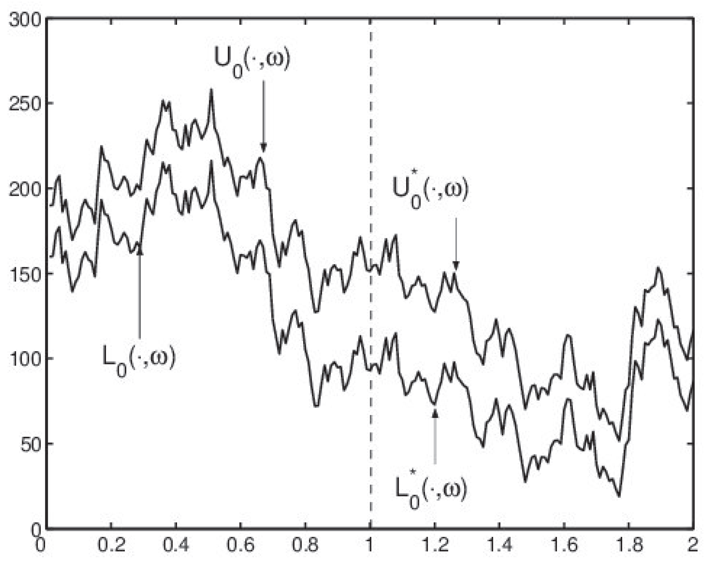
It can be expected that the fed population will expand and the number of individuals will increase, which will cause increasing inaccuracy (fuzziness) in assessing the population density obtained from observations under the microscope. The opposite situation should take place when the population is not fed, because the smaller number of individuals will be conducive to less imprecision (fuzziness) in assessing the number of individuals and thus the density. All this forces the model in the form of a symmetric fuzzy stochastic equation that contain integrals on both sides of the equation. According to our knowledge of the phenomenon under study, the following equation may be an appropriate model

$$x\left(t\right)\oplus (-1)\odot {\int }_0^{t}a\left(s\right)\odot x\left(s\right)ds\oplus ⟨{\int }_0^t\frac{-\sigma }{2}dW\left(s\right)⟩\stackrel{IP.1}{=}{x}_0\oplus {\int }_0^{t}b\left(s\right)\odot x\left(s\right)ds\oplus ⟨{\int }_0^t\frac{\sigma }{2}dW\left(s\right)⟩,$$

where $I=[0,2]$, a and b are some real functions, σ is a real constant, and $x_0$ is a fuzzy set (it could be a fuzzy random variable in general). Of course, this equation can be rewritten as

$$x\left(t\right)\stackrel{IP.1}{=}\left[x_0\oplus {\int }_0^{t}b\left(s\right)\odot x\left(s\right)ds\right]\ominus \left[(-1)\odot {\int }_0^{t}a\left(s\right)\odot x\left(s\right)ds\right]\oplus ⟨{\int }_0^t\sigma dW\left(s\right)⟩,$$

(2)

Assume that it has been established that

$$a\left(t\right)=\left\{\begin{array}{cc}0,& t\in [0,1],\hfill \\ 4t^2-12t+8,& t\in (1,2],\hfill \end{array}\right.b\left(t\right)=\left\{\begin{array}{cc}-4t^2+4t,& t\in [0,1],\hfill \\ 0,& t\in (1,2],\hfill \end{array}\right.\sigma =100.$$

The equation considered above possesses a unique solution x and it is possible to find this solution in explicit form. However, to see the characteristic feature of symmetric Equation (1), we choose a visual presentation of one trajectory of solution support. To this end, let us fix a fuzzy set $x_0$ that will model the initial value “around 175" in such a way that its support ${\left[x_0\right]}_0$ satisfies ${\left[x_0\right]}_0=[160,190]$. Let $L_0(t,\omega )$ and $U_0(t,\omega )$ denote the lower and upper boundary of the solution support, i.e., ${\left[x(t,\omega )\right]}_0=[L_0(t,\omega ),U_0(t,\omega )]$. In Figure 1, we present a simulation of the solution support trajectory by drawing trajectories of $L_0$ and $U_0$.

Figure 1. A trajectory of the support of solution to Equation (2).

The illustration clearly shows that in the first unit of time the length of the interval, which is the support of the solution, increases, while in the next unit of time this length decreases. The length $U_0(t,\omega )-L_0(t,\omega )$ can be an indicator of fuzziness represented in fuzzy set $x(t,\omega )$. Such a change in the type of monotonicity would not be possible without considering a symmetric equation.

Although an explicit form of the solution can be determined for equation in the example above, such a task is usually very difficult, if not impossible. Obtaining a solution to stochastic differential equations in an explicit form is very rare, therefore numerical methods can be helpful to obtain approximate solutions. However, unlike the use of numerical methods in issues of deterministic equations, their use for stochastic equations has some limitations. Namely, for stochastic equations, it is usually not possible to simulate all or almost all trajectories of solution. On the other hand, the use of numerical methods is really legitimate only if we are sure that the equation has a solution and that it is the only one.

In this paper, our aim is to show that the symmetric fuzzy stochastic differential Equation (1) possesses unique solution when the drift coefficients $f,\tilde{f}$ and diffusion coefficients $h^1,h^2\dots ,h^{\ell }$ satisfy a generalized Lipschitz condition, which is obviously weaker than the Lipschitz condition used in [22]. This is justified from a theoretical and practical point of view. First, it is a step in the development of the theory of such equations, and secondly it allows a larger class of mappings from which drift and diffusion equation coefficients can be selected and a unique solution guaranteed.

Here, we collect all the general requirements that we impose on the equation coefficients of (1). In the paper we require that $x_0:\Omega \to \mathcal{F}\left({\mathbb{R}}^d\right)$, $f,\tilde{f}:I\times \Omega \times \mathcal{F}\left({\mathbb{R}}^d\right)\to \mathcal{F}\left({\mathbb{R}}^d\right)$, $h^k:I\times \Omega \times \mathcal{F}\left({\mathbb{R}}^d\right)\to {\mathbb{R}}^d$ ($k=1,2,\dots ,\ell$) satisfy:

(A0)

$x_0\in {\mathcal{L}}^2(\Omega ,{\mathcal{A}}_0,P;\mathcal{F}\left({\mathbb{R}}^d\right))$;

(A1)

the mappings $f,\tilde{f}:(I\times \Omega )\times \mathcal{F}\left({\mathbb{R}}^d\right)\to \mathcal{F}\left({\mathbb{R}}^d\right)$ are $\mathcal{N}\otimes {\mathcal{B}}_{d_{\infty }}|{\mathcal{B}}_{d_{\infty }}$-measurable and $h^1,h^2,\dots ,h^{\ell }:(I\times \Omega )\times \mathcal{F}\left({\mathbb{R}}^d\right)\to {\mathbb{R}}^d$ are $\mathcal{N}\otimes {\mathcal{B}}_{d_{\infty }}|\mathcal{B}\left({\mathbb{R}}^d\right)$-measurable;

(A2)

P-a.a. it holds

$$d_{\infty }^2\left(f(t,\omega ,u),f(t,\omega ,v)\right)\wedge d_{\infty }^2\left(\tilde{f}(t,\omega ,u),\tilde{f}(t,\omega ,v)\right)⩽\xi \left(d_{\infty }^2(u,v)\right),$$

for every $t\in I$ and for any $u,v\in \mathcal{F}\left({\mathbb{R}}^d\right)$, and

$$\parallel h^k(t,\omega ,u)-h^k{(t,\omega ,v)\parallel }^2⩽\xi \left(d_{\infty }^2(u,v)\right),$$

for every $t\in I$, for any $u,v\in \mathcal{F}\left({\mathbb{R}}^d\right)$ and $k=1,2,\dots ,\ell$, where $\xi :{\mathbb{R}}_{+}\to {\mathbb{R}}_{+}$ is a continuous, concave, nondecreasing function such that $\xi \left(0\right)=0$, $\xi \left(a\right)>0$ for $a>0$, and ${\int }_{0^{+}}\frac{da}{\xi \left(a\right)}=\infty$;

(A3)

there exists a constant $C>0$ such that P-a.a. it holds: for every $t\in I$

$$d_{\infty }^2\left(f(t,\omega ,⟨0⟩),⟨0⟩\right)\wedge d_{\infty }^2\left(\tilde{f}(t,\omega ,⟨0⟩),⟨0⟩\right)⩽C,$$

and for every $t\in I$ and $k=1,2,\dots ,\ell$

$$\parallel h^k{(t,\omega ,⟨0⟩)\parallel }^2⩽C;$$

and

(A4)

there exists a constant $\tilde{T}\in (0,T]$ such that for every $n\in \mathbb{N}$ the mappings $y_n:\tilde{I}\times \Omega \to \mathcal{F}\left({\mathbb{R}}^d\right)$, where $\tilde{I}=[0,\tilde{T}]$, described as

$$\begin{array}{cc}{y}_n\left(t\right)\stackrel{[-1,0]P.1}{=}& x_0,\\ y_n\left(t\right)\stackrel{\tilde{I}P.1}{=}& \left[x_0\oplus {\int }_0^t\tilde{f}(s,y_n(s-\frac{1}{n}))ds\right]\ominus \left[(-1)\odot {\int }_0^{t}f(s,y_n(s-\frac{1}{n}))ds\right]\\ & \oplus ⟨\sum _{k=1}^{\ell }{\int }_0^t{h}^k(s,y_n(s-\frac{1}{n}))d{W}^k\left(s\right)⟩\hfill \end{array}$$

are well defined (in particular, the Hukuhara differences do exist).

Let us notice that, if $\xi \left(a\right)=La$, where L is a positive constant, then (A2) reduces to the Lipschitz condition considered in [22]. Therefore, the condition under consideration here is weakened compared to the previous one and extends significantly the set of drift and diffusion mappings that ensure the existence of a unique solution. Some examples of functions $\xi$ different from $\xi \left(a\right)=La$ are known in the literature [29], namely ${\xi }_1$ and ${\xi }_2$ defined as

$$\begin{array}{ccc}\hfill {\xi }_1\left(a\right)& =& alog\left(a^{-1}\right){\mathbf{1}}_{[0,\delta ]}\left(a\right)+[\delta log\left({\delta }^{-1}\right)+{\xi }_1^{\prime }(\delta -)(a-\delta )]{\mathbf{1}}_{(\delta ,\infty )}\left(a\right),\hfill \\ \hfill {\xi }_2\left(a\right)& =& alog\left(a^{-1}\right)loglog\left(a^{-1}\right){\mathbf{1}}_{[0,\delta ]}\left(a\right)+[\delta log\left({\delta }^{-1}\right)loglog\left({\delta }^{-1}\right)+{\xi }_2^{\prime }(\delta -)(a-\delta )]{\mathbf{1}}_{(\delta ,\infty )}\left(a\right),\hfill \end{array}$$

where $\delta \in (0,1)$ is sufficiently small and ${\xi }_i^{\prime }(\delta -)$ ($i=1,2$) denotes left-sided derivative of ${\xi }_i$ at $\delta$.

To prove that symmetric fuzzy stochastic differential equations possess unique solutions under conditions presented above, we use a sequence of successive approximations ${\left\{y_n\right\}}_{n\in \mathbb{N}}$. In what follows, we derive a series of properties of the sequence $\left\{y_n\right\}$. First, we show that $y_n$ is a proper fuzzy stochastic process for every $n\in \mathbb{N}$.

Lemma 3.

Let $x_0,f,\tilde{f}$ and $h^k$ for $k=1,2,\dots ,\ell$ satisfy (A0)–(A4). Then, $y_n:\tilde{I}\times \Omega \to \mathcal{F}\left({\mathbb{R}}^d\right)$ are $d_{\infty }$-continuous, nonanticipating fuzzy stochastic processes that belong to ${\mathcal{L}}^2(\tilde{I}\times \Omega ,\mathcal{N};\mathcal{F}\left({\mathbb{R}}^d\right))$.

Proof. 

Since $x_0\in {\mathcal{L}}^2(\Omega ,{\mathcal{A}}_0,P;\mathcal{F}\left({\mathbb{R}}^d\right))$, we immediately have $\mathbb{E}{d}_{\infty }^2(x_0,⟨0⟩)<\infty$. Denote $M_1=\mathbb{E}{d}_{\infty }^2(x_0,⟨0⟩)$ and let us fix $n\in \mathbb{N}$. We begin with an analysis on the interval $[0,\frac{1}{n}]\cap \tilde{I}$. Let us notice that the mappings

• $[0,\frac{1}{n}]\cap \tilde{I}\times \Omega \ni (s,\omega )\mapsto f(s,\omega ,x_0\left(\omega \right))\in \mathcal{F}\left({\mathbb{R}}^d\right)$,
• $[0,\frac{1}{n}]\cap \tilde{I}\times \Omega \ni (s,\omega )\mapsto \tilde{f}(s,\omega ,x_0\left(\omega \right))\in \mathcal{F}\left({\mathbb{R}}^d\right)$,

are the nonanticipating fuzzy stochastic processes and

• $[0,\frac{1}{n}]\cap \tilde{I}\times \Omega \ni (s,\omega )\mapsto h^k(s,\omega ,x_0\left(\omega \right))\in {\mathbb{R}}^d$ for $k=1,2,\dots ,\ell$

are the single-valued stochastic processes because of measurability Assumption (A1). Further, let us observe that

$$\begin{array}{c}\hfill \mathbb{E}{\int }_{[0,\frac{1}{n}]\cap \tilde{I}}{d}_{\infty }^2(f(s,x_0),⟨0⟩)ds⩽2{\int }_{[0,\frac{1}{n}]\cap \tilde{I}}\mathbb{E}{d}_{\infty }^2(f(s,x_0),f(s,⟨0⟩))ds+2{\int }_{[0,\frac{1}{n}]\cap \tilde{I}}\mathbb{E}{d}_{\infty }^2(f(s,⟨0⟩),⟨0⟩)ds\end{array}$$

and by (A2) and (A3)

$$\begin{array}{c}\hfill \mathbb{E}{\int }_{[0,\frac{1}{n}]\cap \tilde{I}}{d}_{\infty }^2(f(s,x_0),⟨0⟩)ds⩽2{\int }_{[0,\frac{1}{n}]\cap \tilde{I}}\mathbb{E}\xi \left(d_{\infty }^2(x_0,⟨0⟩)\right)ds+\frac{2C}{n}.\end{array}$$

Due to Jensen’s inequality,

$$\begin{array}{c}\hfill \mathbb{E}{\int }_{[0,\frac{1}{n}]\cap \tilde{I}}{d}_{\infty }^2(f(s,x_0),⟨0⟩)ds⩽2{\int }_{[0,\frac{1}{n}]\cap \tilde{I}}\xi \left(\mathbb{E}{d}_{\infty }^2(x_0,⟨0⟩)\right)ds+\frac{2C}{n}⩽\frac{2\xi \left(M_1\right)}{n}+\frac{2C}{n}<\infty \end{array}$$

which means that the process $(s,\omega )\mapsto f(s,\omega ,x_0\left(\omega \right))$ is ${\mathcal{L}}^2$-integrably bounded. Similar calculations show that $(s,\omega )\mapsto \tilde{f}(s,\omega ,x_0\left(\omega \right))$ is ${\mathcal{L}}^2$-integrably bounded as well and $(s,\omega )\mapsto h^k(s,\omega ,x_0\left(\omega \right))$ for $k=1,2,\dots ,\ell$ are square integrable. Hence, by Lemma 1 (i) and (ii), the fuzzy stochastic processes

$$[0,\frac{1}{n}]\cap \tilde{I}\times \Omega \ni (t,\omega )\mapsto {\int }_0^{t}f(s,\omega ,x_0\left(\omega \right))ds\in \mathcal{F}\left({\mathbb{R}}^d\right),$$

$$[0,\frac{1}{n}]\cap \tilde{I}\times \Omega \ni (t,\omega )\mapsto {\int }_0^t\tilde{f}(s,\omega ,x_0\left(\omega \right))ds\in \mathcal{F}\left({\mathbb{R}}^d\right)$$

are nonanticipating, ${\mathcal{L}}^2$-integrably bounded, and $d_{\infty }$-continuous, and obviously the single-valued Itô processes

$$[0,\frac{1}{n}]\cap \tilde{I}\times \Omega \ni (t,\omega )\mapsto \left({\int }_0^t{h}^k(s,x_0)d{W}^k\left(s\right)\right)\left(\omega \right)\in {\mathbb{R}}^d$$

for $k=1,2,\dots ,\ell$ are nonanticipating, square integrable, and continuous.

Since ⊕ and ⊖ are the inner operations in $\mathcal{F}\left({\mathbb{R}}^d\right)$, and the sum and Hukuhara difference of two fuzzy random variables are still fuzzy random variables and in view of (A4), we conclude that

$$\begin{array}{c}\hfill y_n\left(t\right)=\left[x_0\oplus {\int }_0^t\tilde{f}(s,x_0)ds\right]\ominus \left[(-1)\odot {\int }_0^{t}f(s,x_0)ds\right]\oplus ⟨\sum _{k=1}^{\ell }{\int }_0^t{h}^k(s,x_0)d{W}^k\left(s\right)⟩\end{array}$$

is well defined for $t\in [0,\frac{1}{n}]\cap \tilde{I}$ and is nonanticipating, ${\mathcal{L}}^2$-integrably bounded and $d_{\infty }$-continuous fuzzy stochastic process. Now, having $y_n$ defined on the interval $[0,\frac{1}{n}]\cap \tilde{I}$ we can move on to defining it on the second interval $[0,\frac{2}{n}]\cap \tilde{I}$ by following exactly the same steps as above. This procedure is repeated until we reach the right boundary of the interval $\tilde{I}$. □

Below, we state an observation on boundedness of the sequence $\left\{y_n\right\}$.

Lemma 4.

Let $x_0,f,\tilde{f},h^k$ satisfy (A0)–(A4). Then, there exists a positive constant $C_1$ such that for every $n\in \mathbb{N}$

$$\mathbb{E}\underset{t\in \tilde{I}}{sup}{d}_{\infty }^2(y_n\left(t\right),⟨0⟩)⩽C_1.$$

Proof. 

Let us observe that for $t\in \tilde{I}$

$$\begin{array}{ccc}\hfill \mathbb{E}\underset{u\in [0,t]}{sup}{d}_{\infty }^2(y_n\left(u\right),⟨0⟩)& =& \mathbb{E}\underset{u\in [0,t]}{sup}{d}_{\infty }^2(\left[x_0\oplus {\int }_0^u\tilde{f}(s,y_n(s-\frac{1}{n}))ds\right]\ominus \left[(-1)\odot {\int }_0^{u}f(s,y_n(s-\frac{1}{n}))ds\right]\hfill \\ & & \oplus ⟨\sum _{k=1}^{\ell }(-1){\int }_0^u{h}^k(s,y_n(s-\frac{1}{n}))d{W}^k\left(s\right)⟩,⟨0⟩).\hfill \end{array}$$

Now, applying Properties (P4), (P6), and (P5), we get

$$\begin{array}{ccc}\hfill \mathbb{E}\underset{u\in [0,t]}{sup}{d}_{\infty }^2(y_n\left(u\right),⟨0⟩)& ⩽& 8\mathbb{E}{d}_{\infty }^2(x_0,⟨0⟩)+8\mathbb{E}\underset{u\in [0,t]}{sup}{d}_{\infty }^2\left({\int }_0^u\tilde{f}(s,y_n(s-\frac{1}{n}))ds,⟨0⟩\right)\hfill \\ & & +4\mathbb{E}\underset{u\in [0,t]}{sup}{d}_{\infty }^2\left({\int }_0^{u}f(s,y_n(s-\frac{1}{n}))ds,⟨0⟩\right)\hfill \\ & & +2\ell \sum _{k=1}^{\ell }\mathbb{E}\underset{u\in [0,t]}{sup}{∥{\int }_0^u{h}^k(s,y_n(s-\frac{1}{n}))d{W}^k\left(s\right)∥}^2.\hfill \end{array}$$

Further,

$$\begin{array}{ccc}\hfill \mathbb{E}\underset{u\in [0,t]}{sup}{d}_{\infty }^2(y_n\left(u\right),⟨0⟩)& ⩽& 8\mathbb{E}{d}_{\infty }^2(x_0,⟨0⟩)+16\mathbb{E}\underset{u\in [0,t]}{sup}{d}_{\infty }^2\left({\int }_0^u\tilde{f}(s,y_n(s-\frac{1}{n}))ds,{\int }_0^u\tilde{f}(s,⟨0⟩)ds\right)\hfill \\ & & +16\mathbb{E}\underset{u\in [0,t]}{sup}{d}_{\infty }^2\left({\int }_0^u\tilde{f}(s,⟨0⟩)ds,⟨0⟩\right)\hfill \\ & & +8\mathbb{E}\underset{u\in [0,t]}{sup}{d}_{\infty }^2\left({\int }_0^{u}f(s,y_n(s-\frac{1}{n}))ds,{\int }_0^{u}f(s,⟨0⟩)ds\right)\hfill \\ & & +8\mathbb{E}\underset{u\in [0,t]}{sup}{d}_{\infty }^2\left({\int }_0^{u}f(s,⟨0⟩)ds,⟨0⟩\right)\hfill \\ & & +4\ell \sum _{k=1}^{\ell }\mathbb{E}\underset{u\in [0,t]}{sup}{∥{\int }_0^u\left(h^k(s,y_n(s-\frac{1}{n}))-h^k(s,⟨0⟩)\right)d{W}^k\left(s\right)∥}^2\hfill \\ & & +4\ell \sum _{k=1}^{\ell }\mathbb{E}\underset{u\in [0,t]}{sup}{∥{\int }_0^u{h}^k(s,⟨0⟩)d{W}^k\left(s\right)∥}^2.\hfill \end{array}$$

By Lemma 1 and the Doob inequality, we obtain

$$\begin{array}{ccc}\hfill \mathbb{E}\underset{u\in [0,t]}{sup}{d}_{\infty }^2(y_n\left(u\right),⟨0⟩)& ⩽& 8\mathbb{E}{d}_{\infty }^2(x_0,⟨0⟩)+16t\mathbb{E}{\int }_0^t{d}_{\infty }^2\left(\tilde{f}(s,y_n(s-\frac{1}{n})),\tilde{f}(s,⟨0⟩)\right)ds\hfill \\ & & +16t\mathbb{E}{\int }_0^t{d}_{\infty }^2\left(\tilde{f}(s,⟨0⟩),⟨0⟩\right)ds\hfill \\ & & +16t\mathbb{E}{\int }_0^t{d}_{\infty }^2\left(f(s,y_n(s-\frac{1}{n})),f(s,⟨0⟩)\right)ds\hfill \\ & & +16t\mathbb{E}{\int }_0^t{d}_{\infty }^2\left(f(s,⟨0⟩),⟨0⟩\right)ds\hfill \\ & & +16\ell \sum _{k=1}^{\ell }\mathbb{E}{\int }_0^t{∥h^k(s,y_n(s-\frac{1}{n}))-h^k(s,⟨0⟩)∥}^{2}ds\hfill \\ & & +16\ell \sum _{k=1}^{\ell }\mathbb{E}{\int }_0^t{∥h^k(s,⟨0⟩)∥}^{2}ds.\hfill \end{array}$$

By Assumptions (A2) and (A3), we infer that

$$\begin{array}{ccc}\hfill \mathbb{E}\underset{u\in [0,t]}{sup}{d}_{\infty }^2(y_n\left(u\right),⟨0⟩)& ⩽& 8\mathbb{E}{d}_{\infty }^2(x_0,⟨0⟩)+8Ct(3t+2{\ell }^2)\hfill \\ & & +8(3t+2{\ell }^2)\mathbb{E}{\int }_0^t\xi \left(d_{\infty }^2(y_n(s-\frac{1}{n}),⟨0⟩)\right)ds.\hfill \end{array}$$

Since the function $\xi$ is concave, there exist positive constants a and b such that $\xi \left(u\right)⩽a+bu$ for $u⩾0$. Hence

$$\begin{array}{ccc}\hfill \mathbb{E}\underset{u\in [0,t]}{sup}{d}_{\infty }^2(y_n\left(u\right),⟨0⟩)& ⩽& 8\mathbb{E}{d}_{\infty }^2(x_0,⟨0⟩)+8t(a+C)(3t+2{\ell }^2)\hfill \\ & & +8(3t+2{\ell }^2)\mathbb{E}{\int }_0^t\xi \left(d_{\infty }^2(y_n(s-\frac{1}{n}),⟨0⟩)\right)ds.\hfill \end{array}$$

This leads us to

$$\begin{array}{ccc}\hfill \mathbb{E}\underset{u\in [0,t]}{sup}{d}_{\infty }^2(y_n\left(u\right),⟨0⟩)& ⩽& 8\mathbb{E}{d}_{\infty }^2(x_0,⟨0⟩)+8\tilde{T}(a+C)(3\tilde{T}+2{\ell }^2)\hfill \\ & & +8b(3\tilde{T}+2{\ell }^2){\int }_0^t\mathbb{E}\underset{u\in [0,s]}{sup}\xi \left(d_{\infty }^2(y_n\left(u\right),⟨0⟩)\right)ds.\hfill \end{array}$$

Now, applying the Gronwall inequality, we obtain

$$\begin{array}{ccc}\hfill \mathbb{E}\underset{u\in [0,t]}{sup}{d}_{\infty }^2(y_n\left(u\right),⟨0⟩)& ⩽& \left[8\mathbb{E}{d}_{\infty }^2(x_0,⟨0⟩)+8\tilde{T}(a+C)(3\tilde{T}+2{\ell }^2)\right]exp\left\{8b(3\tilde{T}+2{\ell }^2)t\right\}\hfill \end{array}$$

for every $t\in \tilde{I}$. Hence, it follows easily that $\mathbb{E}{sup}_{u\in [0,\tilde{T}]}{d}_{\infty }^2(y_n\left(u\right),⟨0⟩)⩽C_1$, where $C_1=\left[8\mathbb{E}{d}_{\infty }^2(x_0,⟨0⟩)+8\tilde{T}(a+C)(3\tilde{T}+2{\ell }^2)\right]exp\left\{8b(3\tilde{T}+2{\ell }^2)\tilde{T}\right\}$ which ends the proof. □

The next property indicates a uniform Hölder continuity of the sequence $\left\{y_n\right\}$.

Lemma 5.

Let the assumptions of Lemma 4 be satisfied. Then, there exists a positive constant $C_2$ such that for every $n\in \mathbb{N}$ and every $\tau ,t\in \tilde{I}$, $\tau ⩽t$

$$\mathbb{E}{d}_{\infty }^2(y_n\left(t\right),y_n\left(\tau \right))⩽C_2(t-\tau ).$$

Proof. 

Let $t,\tau \in \tilde{I}$ be as in the assumptions. Starting with

$$\begin{array}{ccc}\hfill \mathbb{E}{d}_{\infty }^2(y_n\left(t\right),y_n\left(\tau \right))& =& \mathbb{E}{d}_{\infty }^2(\left[x_0\oplus {\int }_0^t\tilde{f}(s,y_n(s-\frac{1}{n}))ds\right]\ominus \left[(-1)\odot {\int }_0^{t}f(s,y_n(s-\frac{1}{n}))ds\right]\hfill \\ & & \oplus ⟨\sum _{k=1}^{\ell }(-1){\int }_0^t{h}^k(s,y_n(s-\frac{1}{n}))d{W}^k\left(s\right)⟩,\hfill \\ & & \left[x_0\oplus {\int }_0^{\tau }\tilde{f}(s,y_n(s-\frac{1}{n}))ds\right]\ominus \left[(-1)\odot {\int }_0^{\tau }f(s,y_n(s-\frac{1}{n}))ds\right]\hfill \\ & & \oplus ⟨\sum _{k=1}^{\ell }(-1){\int }_0^{\tau }{h}^k(s,y_n(s-\frac{1}{n}))d{W}^k\left(s\right)⟩)\hfill \end{array}$$

and using Properties (P4), (P8), and (P5), we obtain

$$\begin{array}{ccc}\hfill \mathbb{E}{d}_{\infty }^2(y_n\left(t\right),y_n\left(\tau \right))& ⩽& 4\mathbb{E}{d}_{\infty }^2\left({\int }_{\tau }^t\tilde{f}(s,y_n(s-\frac{1}{n}))ds,⟨0⟩\right)+4\mathbb{E}{d}_{\infty }^2\left({\int }_{\tau }^{t}f(s,y_n(s-\frac{1}{n}))ds,⟨0⟩\right)\hfill \\ & & +\ell \sum _{k=1}^{\ell }\mathbb{E}{∥{\int }_{\tau }^t{h}^k(s,y_n(s-\frac{1}{n}))d{W}^k\left(s\right)∥}^2.\hfill \end{array}$$

Due to Lemma 1 and the Itô isometry, we have

$$\begin{array}{ccc}\hfill \mathbb{E}{d}_{\infty }^2(y_n\left(t\right),y_n\left(\tau \right))& ⩽& 4(t-\tau )\mathbb{E}{\int }_{\tau }^t{d}_{\infty }^2\left(\tilde{f}(s,y_n(s-\frac{1}{n})),⟨0⟩\right)ds\hfill \\ & & +4(t-\tau )\mathbb{E}{\int }_{\tau }^t{d}_{\infty }^2\left(f(s,y_n(s-\frac{1}{n})),⟨0⟩\right)ds\hfill \\ & & +\ell \sum _{k=1}^{\ell }\mathbb{E}{\int }_{\tau }^t{∥h^k(s,y_n(s-\frac{1}{n}))∥}^{2}ds\hfill \end{array}$$

and further

$$\begin{array}{ccc}\hfill \mathbb{E}{d}_{\infty }^2(y_n\left(t\right),y_n\left(\tau \right))& ⩽& 8(t-\tau )\mathbb{E}{\int }_{\tau }^t{d}_{\infty }^2\left(\tilde{f}(s,y_n(s-\frac{1}{n})),\tilde{f}(s,⟨0⟩)\right)ds\hfill \\ & & +8(t-\tau )\mathbb{E}{\int }_{\tau }^t{d}_{\infty }^2\left(\tilde{f}(s,⟨0⟩),⟨0⟩\right)ds\hfill \\ & & +8(t-\tau )\mathbb{E}{\int }_{\tau }^t{d}_{\infty }^2\left(f(s,y_n(s-\frac{1}{n})),f(s,⟨0⟩)\right)ds\hfill \\ & & +8(t-\tau )\mathbb{E}{\int }_{\tau }^t{d}_{\infty }^2\left(f(s,⟨0⟩),⟨0⟩\right)ds\hfill \\ & & +2\ell \sum _{k=1}^{\ell }\mathbb{E}{\int }_{\tau }^t{∥h^k(s,y_n(s-\frac{1}{n}))-h^k(s,⟨0⟩)∥}^{2}ds+2\ell \sum _{k=1}^{\ell }\mathbb{E}{\int }_{\tau }^t{∥h^k(s,⟨0⟩)∥}^{2}ds.\hfill \end{array}$$

Invoking Assumptions (A2) and (A3),

$$\begin{array}{ccc}\hfill \mathbb{E}{d}_{\infty }^2(y_n\left(t\right),y_n\left(\tau \right))& ⩽& \left(16(t-\tau )+2{\ell }^2\right)\left(\mathbb{E}{\int }_{\tau }^t\xi \left(d_{\infty }^2(y_n(s-\frac{1}{n}),⟨0⟩)\right)ds+C(t-\tau )\right)\hfill \\ & ⩽& \left(16\tilde{T}+2{\ell }^2\right)\left({\int }_{\tau }^t\mathbb{E}\xi \left(d_{\infty }^2(y_n(s-\frac{1}{n}),⟨0⟩)\right)ds+C(t-\tau )\right).\hfill \end{array}$$

By Jensen’s inequality and nondecreasiness of $\xi$,

$$\begin{array}{ccc}\hfill \mathbb{E}{d}_{\infty }^2(y_n\left(t\right),y_n\left(\tau \right))& ⩽& \left(16\tilde{T}+2{\ell }^2\right)\left({\int }_{\tau }^t\xi \left(\mathbb{E}{d}_{\infty }^2(y_n(s-\frac{1}{n}),⟨0⟩)\right)ds+C(t-\tau )\right)\hfill \\ & ⩽& \left(16\tilde{T}+2{\ell }^2\right)\left({\int }_{\tau }^t\xi \left(\mathbb{E}\underset{u\in \tilde{I}}{sup}{d}_{\infty }^2(y_n\left(u\right),⟨0⟩)\right)ds+C(t-\tau )\right).\hfill \end{array}$$

Applying Lemma 4, we obtain

$$\mathbb{E}{d}_{\infty }^2(y_n\left(t\right),y_n\left(\tau \right))⩽C_2(t-\tau ),$$

where $C_2=(16\tilde{T}+2{\ell }^2)\left(\xi \right(C_1)+C)$.

Lemma 6.

Let the assumptions of Lemma 4 be satisfied. Then,

$$\mathbb{E}\underset{t\in \tilde{I}}{sup}{d}_{\infty }^2(y_n\left(t\right),y_i\left(t\right))⟶0,asn,i\to \infty .$$

Proof. 

Let us fix $n,i\in \mathbb{N}$. Without loss of generality, we may assume that $n>i$. Observe that, for $t\in \tilde{I}$, we have

$$\begin{array}{cc}\mathbb{E}\underset{u\in [0,t]}{sup}{d}_{\infty }^2(y_n\left(u\right),y_i\left(u\right))\hfill & \\ & ⩽2\mathbb{E}\underset{u\in [0,t]}{sup}{d}_{\infty }^2(\left[x_0\oplus {\int }_0^u\tilde{f}(s,y_n(s-\frac{1}{n}))ds\right]\ominus \left[(-1)\odot {\int }_0^{u}f(s,y_n(s-\frac{1}{n}))ds\right],\hfill \\ & \left[x_0\oplus {\int }_0^u\tilde{f}(s,y_i(s-\frac{1}{i}))ds\right]\ominus \left[(-1)\odot {\int }_0^{u}f(s,y_i(s-\frac{1}{i}))ds\right])\hfill \\ & +2\ell \sum _{k=1}^{\ell }\mathbb{E}\underset{u\in [0,t]}{sup}{∥{\int }_0^u\left(h^k(s,y_n(s-\frac{1}{n}))-h^k(s,y_i(s-\frac{1}{i}))\right)d{W}^k\left(s\right)∥}^2.\hfill \end{array}$$

Now, using Property (P8) together with Lemma 1 and Doob’s inequality, we obtain

$$\begin{array}{cc}\hfill \mathbb{E}\underset{u\in [0,t]}{sup}{d}_{\infty }^2(y_n\left(u\right),y_i\left(u\right))& ⩽4t\mathbb{E}{\int }_0^t{d}_{\infty }^2\left(\tilde{f}(s,y_n(s-\frac{1}{n})),\tilde{f}(s,y_i(s-\frac{1}{i}))\right)ds\hfill \\ & +4t\mathbb{E}{\int }_0^t{d}_{\infty }^2\left(f(s,y_n(s-\frac{1}{n})),f(s,y_i(s-\frac{1}{i}))\right)ds\hfill \\ & +8\ell \sum _{k=1}^{\ell }\mathbb{E}{\int }_0^t{∥h^k(s,y_n(s-\frac{1}{n}))-h^k(s,y_i(s-\frac{1}{i}))∥}^{2}ds,\hfill \end{array}$$

and further

$$\begin{array}{cc}\hfill \mathbb{E}\underset{u\in [0,t]}{sup}{d}_{\infty }^2(y_n\left(u\right),y_i\left(u\right))& ⩽8t\mathbb{E}{\int }_0^t{d}_{\infty }^2\left(\tilde{f}(s,y_n(s-\frac{1}{n})),\tilde{f}(s,y_i(s-\frac{1}{n}))\right)ds\hfill \\ & +8t\mathbb{E}{\int }_0^t{d}_{\infty }^2\left(\tilde{f}(s,y_i(s-\frac{1}{n})),\tilde{f}(s,y_i(s-\frac{1}{i}))\right)ds\hfill \\ & +8t\mathbb{E}{\int }_0^t{d}_{\infty }^2\left(f(s,y_n(s-\frac{1}{n})),f(s,y_i(s-\frac{1}{n}))\right)ds\hfill \\ & +8t\mathbb{E}{\int }_0^t{d}_{\infty }^2\left(f(s,y_i(s-\frac{1}{n})),f(s,y_i(s-\frac{1}{i}))\right)ds\hfill \\ & +16\ell \sum _{k=1}^{\ell }\mathbb{E}{\int }_0^t{∥h^k(s,y_n(s-\frac{1}{n}))-h^k(s,y_i(s-\frac{1}{n}))∥}^{2}ds\hfill \\ & +16\ell \sum _{k=1}^{\ell }\mathbb{E}{\int }_0^t{∥h^k(s,y_i(s-\frac{1}{n}))-h^k(s,y_i(s-\frac{1}{i}))∥}^{2}ds,\hfill \end{array}$$

Assumption (A2) and Jensen’s inequality lead us to

$$\begin{array}{ccc}\hfill \mathbb{E}\underset{u\in [0,t]}{sup}{d}_{\infty }^2(y_n\left(u\right),y_i\left(u\right))& ⩽& 16(t+{\ell }^2){\int }_0^t\xi \left(\mathbb{E}\underset{u\in [0,s]}{sup}{d}_{\infty }^2(y_n\left(u\right),y_i\left(u\right))\right)ds\hfill \\ & & +16(t+{\ell }^2){\int }_0^t\xi \left(\mathbb{E}{d}_{\infty }^2(y_i(s-\frac{1}{n}),y_i(s-\frac{1}{i}))\right)ds.\hfill \end{array}$$

By Lemma 5, we get

$$\begin{array}{ccc}\hfill \mathbb{E}\underset{u\in [0,t]}{sup}{d}_{\infty }^2(y_n\left(u\right),y_i\left(u\right))& ⩽& C_3{\int }_0^t\xi \left(\mathbb{E}\underset{u\in [0,s]}{sup}{d}_{\infty }^2(y_n\left(u\right),y_i\left(u\right))\right)ds\hfill \\ & & +C_3\tilde{T}\xi \left(C_2(\frac{1}{i}-\frac{1}{n})\right),\hfill \end{array}$$

where $C_3=16(\tilde{T}+{\ell }^2)$. Applying Lemma 2, we have

$$\begin{array}{c}\hfill \mathbb{E}\underset{u\in [0,t]}{sup}{d}_{\infty }^2(y_n\left(u\right),y_i\left(u\right))⩽J^{-1}(J(C_3\tilde{T}\xi \left(C_2(\frac{1}{i}-\frac{1}{n})\right)+C_{3}t)\end{array}$$

for every $t\in \tilde{I}$. Owing to Lemma 2 and properties of function J from this lemma, we obtain

$$\underset{n,i\to \infty }{lim}{J}^{-1}(J(C_3\tilde{T}\xi \left(C_2(\frac{1}{i}-\frac{1}{n})\right)+C_3\tilde{T})=0.$$

This allows us to infer that $\underset{n,i\to \infty }{lim}\mathbb{E}{sup}_{t\in \tilde{I}}{d}_{\infty }^2(y_n\left(t\right),y_i\left(t\right))=0$. □

As mentioned above, Conditions (A0)–(A4) assure the existence of a unique solution to Equation (1). This fact, written below, constitutes a first main result of the paper and the the properties listed above are helpful in proving it. Although the method of proving is already signaled in [23], we present it fully here for the convenience of the reader and for completeness.

Theorem 1.

Let $x_0:\Omega \to \mathcal{F}\left({\mathbb{R}}^d\right)$, $f,\tilde{f}:(I\times \Omega )\times \mathcal{F}\left({\mathbb{R}}^d\right)\to \mathcal{F}\left({\mathbb{R}}^d\right)$ and $h^k:(I\times \Omega )\times \mathcal{F}\left({\mathbb{R}}^d\right)\to {\mathbb{R}}^d$ ($k=1,2,\dots ,\ell$) satisfy (A0)–(A4). Then, Equation (1) possesses a unique solution $x:\widehat{I}\times \Omega \to \mathcal{F}\left({\mathbb{R}}^d\right)$.

Proof. 

Let us observe that owing to Lemma 6

$$\underset{n,i\to \infty }{lim}{\rho }^2(y_n\left(t\right),y_i\left(t\right))=0\mathrm{for}\mathrm{every}t\in \tilde{I},$$

where $\rho (x,y)={\left[\mathbb{E}{d}_{\infty }^2(x,y)\right]}^{1/2}$. Since $({\mathcal{L}}^2(\Omega ,{\mathcal{A}}_t,P;\mathcal{F}\left({\mathbb{R}}^d\right)),\rho )$ is a complete metric space, we claim that for every $t\in \tilde{I}$ there exists a unique fuzzy random variable $x_t\in {\mathcal{L}}^2(\Omega ,{\mathcal{A}}_t,P;\mathcal{F}\left({\mathbb{R}}^d\right))$ such that

$$\underset{n\to \infty }{lim}\rho (y_n\left(t\right),x_t)=0.$$

Let us define a fuzzy stochastic process $x:\tilde{I}\times \Omega \to \mathcal{F}\left({\mathbb{R}}^d\right)$ as $x(t,\omega )=x_t\left(\omega \right)$. Then, the fuzzy stochastic process x is $\left\{{\mathcal{A}}_t\right\}$-adapted. Due to the Markov inequality we obtain that for every $\epsilon >0$

$$\underset{n,i\to \infty }{lim}P\left(\underset{t\in \tilde{I}}{sup}{d}_{\infty }(y_n\left(t\right),y_i\left(t\right))>\epsilon \right)=0.$$

Hence, we can infer that there exists a subsequence $\left\{y_{n_{\ell }}(·,·)\right\}$ of the sequence $\left\{y_n(·,·)\right\}$ such that

$$\underset{\ell \to \infty }{lim}\underset{t\in \tilde{I}}{sup}{d}_{\infty }(y_{n_{\ell }}\left(t\right),x\left(t\right))\stackrel{P.1}{=}0.$$

Thus, the process x is $d_{\infty }$-continuous and consequently it is measurable. Since x is also $\left\{{\mathcal{A}}_t\right\}$-adapted, it is nonanticipating. In addition, since $x\left(t\right)\in {\mathcal{L}}^2(\Omega ,{\mathcal{A}}_t,P;\mathcal{F}\left({\mathbb{R}}^d\right))$ for every $t\in \tilde{I}$, we have

$$\mathbb{E}{\int }_{\tilde{I}}{d}_{\infty }^2(x\left(t\right),⟨0⟩)dt⩽\tilde{T}\underset{t\in \tilde{I}}{sup}\mathbb{E}{d}_{\infty }^2(x\left(t\right),⟨0⟩)<\infty .$$

This implies that $x\in {\mathcal{L}}^2(\tilde{I}\times \Omega ,\mathcal{N};\mathcal{F}\left({\mathbb{R}}^d\right))$. Moreover, applying Lemma 4, we infer that

$$\mathbb{E}\underset{t\in \tilde{I}}{sup}{d}_{\infty }^2(x\left(t\right),⟨0⟩)⩽C_1.$$

We can also infer that

$$\underset{\ell \to \infty }{lim}\mathbb{E}\underset{t\in \tilde{I}}{sup}{d}_{\infty }^2(y_{n_{\ell }}\left(t\right),x\left(t\right))=0.$$

(3)

In what follows, we show that x is a solution to Equation (1). To this aim, let us observe that

$$\begin{array}{c}\mathbb{E}\underset{t\in \tilde{I}}{sup}{d}_{\infty }^2\left(x\left(t\right),\left[x_0\oplus {\int }_0^t\tilde{f}(s,x\left(s\right))ds\right]\ominus \left[(-1)\odot {\int }_0^{t}f(s,x\left(s\right))ds\right)\right]\oplus ⟨\sum _{k=1}^{\ell }{\int }_0^t{h}^k(s,x\left(s\right))d{W}^k\left(s\right)⟩)\hfill \\ ⩽2Q_{\ell }+2P_{\ell },\hfill \end{array}$$

where

$$Q_{\ell }=\mathbb{E}\underset{t\in \tilde{I}}{sup}{d}_{\infty }^2\left(y_{n_{\ell }}\left(t\right),x\left(t\right)\right)$$

and

$$\begin{array}{ccc}\hfill P_{\ell }& =\hfill & \mathbb{E}\underset{t\in \tilde{I}}{sup}{d}_{\infty }^2(\left[x_0\oplus {\int }_0^t\tilde{f}(s,y_{n_{\ell }}(s-\frac{1}{n_{\ell }}))ds\right]\ominus \left[(-1)\odot {\int }_0^{t}f(s,y_{n_{\ell }}(s-\frac{1}{n_{\ell }}))ds\right]\hfill \\ & & \oplus ⟨\sum _{k=1}^{\ell }{\int }_0^t{h}^k(s,y_{n_{\ell }}(s-\frac{1}{n_{\ell }}))d{W}^k\left(s\right)⟩,\left[x_0\oplus {\int }_0^t\tilde{f}(s,x\left(s\right))ds\right]\hfill \\ & & \ominus \left[(-1)\odot {\int }_0^{t}f(s,x\left(s\right))ds\right]\oplus ⟨\sum _{k=1}^{\ell }{\int }_0^t{h}^k(s,x\left(s\right))d{W}^k\left(s\right)⟩).\hfill \end{array}$$

By Equation (3), the expression $Q_{\ell }$ converges to zero as ℓ goes to infinity, and it can be verified that

$$P_{\ell }⩽C_4\mathbb{E}{\int }_0^{\tilde{T}}\xi \left(d_{\infty }^2(y_{n_{\ell }}(s-\frac{1}{n_{\ell }}),y_{n_{\ell }}\left(s\right))\right)ds+C_4\mathbb{E}{\int }_0^{\tilde{T}}\xi \left(d_{\infty }^2(y_{n_{\ell }}\left(s\right),x\left(s\right))\right)ds,$$

where $C_4=16(\tilde{T}+1)$. Thus,

$$P_{\ell }⩽C_4{\int }_0^{\tilde{T}}\xi \left(\mathbb{E}{d}_{\infty }^2(y_{n_{\ell }}(s-\frac{1}{n_{\ell }}),y_{n_{\ell }}\left(s\right))\right)ds+C_4{\int }_0^{\tilde{T}}\xi \left(\mathbb{E}\underset{u\in \tilde{I}}{sup}{d}_{\infty }^2(y_{n_{\ell }}\left(u\right),x\left(u\right))\right)ds.$$

Applying Lemma 5, we obtain

$$P_{\ell }⩽C_4\tilde{T}\xi \left(\frac{C_2}{n_{\ell }}\right)+C_4\tilde{T}\xi \left(\mathbb{E}\underset{u\in \tilde{I}}{sup}{d}_{\infty }^2(y_{n_{\ell }}\left(u\right),x\left(u\right))\right).$$

By the properties of $\xi$ and in view of Equation (3), the right-hand side of the latter inequality converges to zero. Thus,

$$\begin{array}{c}\mathbb{E}\underset{t\in \tilde{I}}{sup}{d}_{\infty }^2(x\left(t\right),\left[x_0\oplus {\int }_0^t\tilde{f}(s,x\left(s\right))ds\right]\ominus \left[(-1)\odot {\int }_0^{t}f(s,x\left(s\right))ds\right]\hfill \\ \oplus ⟨\sum _{k=1}^{\ell }{\int }_0^t{h}^k(s,x\left(s\right))d{W}^k\left(s\right)⟩)=0\hfill \end{array}$$

which implies that

$$\begin{array}{c}\underset{u\in \tilde{I}}{sup}{d}_{\infty }(x\left(u\right),\left[x_0\oplus {\int }_0^t\tilde{f}(s,x\left(s\right))ds\right]\ominus \left[(-1)\odot {\int }_0^{t}f(s,x\left(s\right))ds\right]\\ \oplus ⟨\sum _{k=1}^{\ell }{\int }_0^t{h}^k(s,x\left(s\right))d{W}^k\left(s\right)⟩)\stackrel{P.1}{=}0.\end{array}$$

This shows that x is a solution to Equation (1). Now, we prove that x is a unique solution. To this end, assume that $y:\tilde{I}\times \Omega \to \mathcal{F}\left({\mathbb{R}}^d\right)$ is another solution to Equation (1). Then, for $t\in \tilde{I}$ we have

$$\begin{array}{ccc}\hfill \mathbb{E}\underset{u\in [0,t]}{sup}{d}_{\infty }^2\left(x\left(u\right),y\left(u\right)\right)& ⩽\hfill & 4t\mathbb{E}{\int }_0^t{d}_{\infty }^2(\tilde{f}(s,x\left(s\right)),\tilde{f}(s,y\left(s\right)))ds\hfill \\ & & +4t\mathbb{E}{\int }_0^t{d}_{\infty }^2(f(s,x\left(s\right)),f(s,y\left(s\right)))ds\hfill \\ & & +8\ell \sum _{k=1}^{\ell }\mathbb{E}{\int }_0^t{∥h^k(s,x\left(s\right))-h^k(s,y\left(s\right))∥}^{2}ds.\hfill \end{array}$$

Hence,

$$\mathbb{E}\underset{u\in [0,t]}{sup}{d}_{\infty }^2\left(x\left(u\right),y\left(u\right)\right)⩽8(\tilde{T}+{\ell }^2){\int }_0^t\xi \left(\mathbb{E}\underset{u\in [0,s]}{sup}{d}_{\infty }^2(x\left(s\right),y\left(s\right))\right)ds.$$

Invoking Lemma 2, we get

$$\mathbb{E}\underset{u\in [0,t]}{sup}{d}_{\infty }^2\left(x\left(u\right),y\left(u\right)\right)⩽0\mathrm{for}\mathrm{every}t\in \tilde{I}.$$

Therefore,

$$\mathbb{E}\underset{u\in \tilde{I}}{sup}{d}_{\infty }^2\left(x\left(u\right),y\left(u\right)\right)=0,$$

which implies that

$$\underset{u\in \tilde{I}}{sup}{d}_{\infty }\left(x\left(u\right),y\left(u\right)\right)\stackrel{P.1}{=}0.$$

This proves uniqueness of the solution x. The proof is completed. □

4. Stability of Solution

In this section, we examine a certain basic type of stability of solutions to symmetric fuzzy stochastic differential equations in order to show that the theory of such equations with the generalized Lipschitz condition is well-posed. By stability, we mean here an insensitivity of solution to small changes in equation data, i.e., initial value or diffusion or drift coefficients. It is obvious that this kind of stability must be ensured for potential practical applications, because in practice, due to technological limitations and the lack of precision of measurements and imprecision of human knowledge, an inaccurate model of initial value or drift or diffusion is most often available. However, assuming that given equation data have been determined as best as possible, i.e. they are very close to actual data, the stability is to ensure closeness of solution of equation with disturbed data and solution of equation that actually corresponds to studied phenomenon. Therefore, slight data disturbances will not cause big changes in solutions.

Let us consider two symmetric fuzzy stochastic differential equations. The first one is exactly Equation (1), the second one is

$$z\left(t\right)\stackrel{IP.1}{=}\left[z_0\oplus {\int }_0^t\tilde{f}(s,z\left(s\right))ds\right]\ominus \left[(-1)\odot {\int }_0^{t}f(s,z\left(s\right))ds\right]\oplus ⟨\sum _{k=1}^{\ell }{\int }_0^t{h}^k(s,z\left(s\right))d{W}^k\left(s\right)⟩$$

(4)

and let $x,z:\tilde{I}\times \Omega \to \mathcal{F}\left({\mathbb{R}}^d\right)$ denote solutions to Equations (1) and (4) (provided they exist), respectively. It is easy to observe that both equations differ only in the initial value, the remaining data are identical. The essence of current research is to justify the stability of the solution relative to small changes in the initial value.

Theorem 2.

Let the fuzzy random variables $x_0,z_0$ satisfy Condition (A0). Suppose $f,\tilde{f},h^1,h^2,\dots ,h^{\ell }$ satisfy (A1)–(A3). Assume that the condition (A4) is satisfied by $x_0,f,\tilde{f},h^1,h^2,\dots ,h^{\ell }$ and $z_0,f,\tilde{f},h^1,h^2,\dots ,h^{\ell }$ with the same constant $\tilde{T}\in (0,T]$. Then, the unique solutions $x,z:\tilde{I}\times \Omega \to \mathcal{F}\left({\mathbb{R}}^d\right)$ to Equations (1) and (4) satisfy

$$\mathbb{E}\underset{t\in \tilde{I}}{sup}{d}_{\infty }^2\left(x\left(t\right),z\left(t\right)\right)⩽J^{-1}\left(J\left(8\mathbb{E}{d}_{\infty }^2(x_0,z_0)\right)+(12\tilde{T}+8{\ell }^2)\tilde{T}\right),$$

where the function J is as in Lemma 2 and $J^{-1}$ is its inverse.

Proof. 

Owing to Theorem 1, the unique solutions $x,z$ to Equations (1) and (4) exist. For $t\in \tilde{I}$, one gets

$$\begin{array}{ccc}\hfill \mathbb{E}\underset{u\in [0,t]}{sup}{d}_{\infty }^2\left(x\left(u\right),z\left(u\right)\right)& ⩽\hfill & 2\mathbb{E}\underset{u\in [0,t]}{sup}{d}_{\infty }^2(\left[x_0\oplus {\int }_0^u\tilde{f}(s,x\left(s\right))ds\right]\ominus \left[(-1)\odot {\int }_0^{u}f(s,x\left(s\right))ds\right],\hfill \\ & & \left[z_0\oplus {\int }_0^u\tilde{f}(s,z\left(s\right))ds\right]\ominus \left[(-1)\odot {\int }_0^{u}f(s,z\left(s\right))ds\right]\hfill \\ & & +2\mathbb{E}\underset{u\in [0,t]}{sup}{∥\sum _{k=1}^{\ell }{\int }_0^u\left(h^k(s,x\left(s\right))-h^k(s,z\left(s\right))\right)d{W}^k\left(s\right)∥}^2.\hfill \end{array}$$

Applying Lemma 1 and the Doob inequality, we get

$$\begin{array}{ccc}\hfill \mathbb{E}\underset{u\in [0,t]}{sup}{d}_{\infty }^2\left(x\left(u\right),z\left(u\right)\right)& ⩽& 8\mathbb{E}{d}_{\infty }^2(x_0,z_0)+8t\mathbb{E}{\int }_0^t{d}_{\infty }^2(\tilde{f}(s,x\left(s\right)),\tilde{f}(s,z\left(s\right)))ds\hfill \\ & & +4t\mathbb{E}{\int }_0^t{d}_{\infty }^2(f(s,x\left(s\right)),f(s,z\left(s\right)))ds\hfill \\ & & +8\ell \sum _{k=1}^{\ell }\mathbb{E}{\int }_0^t{\parallel h^k(s,x\left(s\right))-h^k(s,z\left(s\right))\parallel }^{2}ds.\hfill \end{array}$$

By Assumption (A2) and Jensen’s inequality,

$$\begin{array}{ccc}\hfill \mathbb{E}\underset{u\in [0,t]}{sup}{d}_{\infty }^2\left(x\left(u\right),z\left(u\right)\right)& ⩽& 8\mathbb{E}{d}_{\infty }^2(x_0,z_0)+(12t+8{\ell }^2){\int }_0^t\xi \left(\mathbb{E}\underset{u\in [0,s]}{sup}{d}_{\infty }^2\left(x\left(u\right),z\left(u\right)\right)\right)ds.\hfill \end{array}$$

Finally, by Lemma 2,

$$\mathbb{E}\underset{u\in [0,t]}{sup}{d}_{\infty }^2\left(x\left(u\right),y\left(u\right)\right)⩽J^{-1}\left(J\left(8\mathbb{E}{d}_{\infty }^2(x_0,z_0)\right)+(12t+8{\ell }^2)t\right)\mathrm{for}\mathrm{every}t\in \tilde{I}$$

which completes the proof. □

From the above theorem, it can be seen that small changes in the initial value cannot cause large changes in solutions. This allows us to infer the property of continuous dependence of solution with respect to the initial value. Indeed, consider Equation (1) and

$$\begin{array}{ccc}\hfill z_n\left(t\right)& \stackrel{IP.1}{=}& \left[z_0^{\left(n\right)}\oplus {\int }_0^t\tilde{f}(s,z_n\left(s\right))ds\right]\ominus \left[(-1)\odot {\int }_0^{t}f(s,z_n\left(s\right))ds\right]\hfill \\ & & \oplus ⟨\sum _{k=1}^{\ell }{\int }_0^t{h}^k(s,z_n\left(s\right))d{W}^k\left(s\right)⟩,n\in \mathbb{N}.\hfill \end{array}$$

(5)

Corollary 1.

Let the fuzzy random variables $x_0,z_0^{\left(1\right)},z_0^{\left(2\right)},\dots$ satisfy (A0). Let $f,\tilde{f},h^1,h^2,\dots ,h^{\ell }$ satisfy (A1)–(A3). Suppose that Condition (A4) is satisfied with the same constant $\tilde{T}$ for each of systems $(x_0,f,\tilde{f},h^1,h^2,\dots ,h^{\ell })$, $(z_0^{\left(1\right)},f,\tilde{f},h^1,h^2,\dots ,h^{\ell })$, $(z_0^{\left(2\right)},f,\tilde{f},h^1,h^2,\dots ,h^{\ell }),\dots$ Assume that

$$\mathbb{E}{d}_{\infty }^2(z_0^{\left(n\right)},x_0)\to 0\mathrm{as}n\to \infty .$$

Then, for the unique solution $x:\tilde{I}\times \Omega \to \mathcal{F}\left({\mathbb{R}}^d\right)$ to Equation (1) and the unique solutions $z_n:\tilde{I}\times \Omega \to \mathcal{F}\left({\mathbb{R}}^d\right)$ to Equation (5), we have

$$\mathbb{E}\underset{t\in \tilde{I}}{sup}{d}_{\infty }^2(z_n\left(t\right),x\left(t\right))\to 0\mathrm{as}n\to \infty .$$

Further analysis is related to examining the impact on the solution resulting from changes in drift and diffusion coefficients. Hence, we consider Equation (1) and

$$\begin{array}{ccc}\hfill z\left(t\right)& \stackrel{IP.1}{=}\hfill & \left[x_0\oplus {\int }_0^t\tilde{p}(s,z\left(s\right))ds\right]\ominus \left[(-1)\odot {\int }_0^{t}p(s,z\left(s\right))ds\right]\hfill \\ & & \oplus ⟨\sum _{k=1}^{\ell }{\int }_0^t{q}^k(s,z\left(s\right))d{W}^k\left(s\right)⟩\hfill \end{array}$$

(6)

to investigate continuous dependence of solution to Equation (1) with respect to coefficients $f,\tilde{f}$ and $h^k$’s. Let $x,z:\tilde{I}\times \Omega \to \mathcal{F}\left({\mathbb{R}}^d\right)$ denote solutions to Equations (1) and (6), respectively.

Theorem 3.

Let the fuzzy random variable $x_0$ satisfy (A0). Let the systems $(f,\tilde{f},h^1,h^2,\dots ,h^{\ell })$ and $(p,\tilde{p},q^1,q^2,\dots ,q^{\ell })$ satisfy (A1)–(A3). Assume that Condition (A4) is satisfied with the same constant $\tilde{T}\in (0,T]$ for both systems $(x_0,f,\tilde{f},h^1,h^2,\dots ,h^{\ell })$ and $(x_0,p,\tilde{p},q^1,q^2,\dots ,q^{\ell })$. Then, for the unique solution $x:\tilde{I}\times \Omega \to \mathcal{F}\left({\mathbb{R}}^d\right)$ to Equation (1) and the unique solution $z:\tilde{I}\times \Omega \to \mathcal{F}\left({\mathbb{R}}^d\right)$ to Equation (6), we have

$$\mathbb{E}\underset{t\in \tilde{I}}{sup}{d}_{\infty }^2\left(z\left(t\right),x\left(t\right)\right)⩽J^{-1}\left(J\left(c\right)+16\tilde{T}(\tilde{T}+{\ell }^2)\right),$$

where

$$\begin{array}{ccc}\hfill c& =& 8\tilde{T}\mathbb{E}{\int }_{\tilde{I}}{d}_{\infty }^2(\tilde{p}(t,x\left(t\right)),\tilde{f}(t,x\left(t\right)))dt+8\tilde{T}\mathbb{E}{\int }_{\tilde{I}}{d}_{\infty }^2(p(t,x\left(t\right)),f(t,x\left(t\right)))dt\hfill \\ & & +16\ell \sum _{k=1}^{\ell }\mathbb{E}{\int }_{\tilde{I}}{\parallel q^k(t,x\left(t\right))-h^k(t,x\left(t\right))\parallel }^{2}dt\hfill \end{array}$$

and the function J is as in Lemma 2 and $J^{-1}$ is its inverse.

Proof. 

The existence of the unique solutions x to Equation (1) and z to Equation (6) is ensured by Theorem 1. For $t\in \tilde{I}$, we have

$$\begin{array}{cc}\mathbb{E}\underset{u\in [0,t]}{sup}{d}_{\infty }^2\left(z\left(u\right),x\left(u\right)\right)\hfill & \\ & ⩽4t\mathbb{E}{\int }_0^t{d}_{\infty }^2(\tilde{p}(s,z\left(s\right)),\tilde{f}(s,x\left(s\right)))ds+4t\mathbb{E}{\int }_0^t{d}_{\infty }^2(p(s,z\left(s\right)),f(s,x\left(s\right)))ds\hfill \\ & +8\ell \sum _{k=1}^{\ell }\mathbb{E}{\int }_0^t{\parallel q^k(s,z\left(s\right))-h^k(s,x\left(s\right))\parallel }^{2}ds\hfill \\ & ⩽8t\mathbb{E}{\int }_0^t{d}_{\infty }^2(\tilde{p}(s,z\left(s\right)),\tilde{p}(s,x\left(s\right)))ds+8t\mathbb{E}{\int }_0^t{d}_{\infty }^2(\tilde{p}(s,x\left(s\right)),\tilde{f}(s,x\left(s\right)))ds\hfill \\ & +8t\mathbb{E}{\int }_0^t{d}_{\infty }^2(p(s,z\left(s\right)),p(s,x\left(s\right)))ds+8t\mathbb{E}{\int }_0^t{d}_{\infty }^2(p(s,x\left(s\right)),f(s,x\left(s\right)))ds\hfill \\ & +16\ell \sum _{k=1}^{\ell }\mathbb{E}{\int }_0^t\parallel q^k(s,z\left(s\right))-q^k{(s,x\left(s\right))\parallel }^{2}ds+16\ell \sum _{k=1}^{\ell }\mathbb{E}{\int }_0^t{\parallel q^k(s,x\left(s\right))-h^k(s,x\left(s\right))\parallel }^{2}ds\hfill \\ & ⩽c+16(t+{\ell }^2){\int }_0^t\xi \left(\mathbb{E}\underset{u\in [0,s]}{sup}{d}_{\infty }^2(z\left(u\right),x\left(u\right))\right)ds,\hfill \end{array}$$

where

$$\begin{array}{ccc}\hfill c& =\hfill & 8\tilde{T}\mathbb{E}{\int }_{\tilde{I}}{d}_{\infty }^2(\tilde{p}(t,x\left(t\right)),\tilde{f}(t,x\left(t\right)))dt+8\tilde{T}\mathbb{E}{\int }_{\tilde{I}}{d}_{\infty }^2(p(t,x\left(t\right)),f(t,x\left(t\right)))dt\hfill \\ & & +16\ell \sum _{k=1}^{\ell }\mathbb{E}{\int }_{\tilde{I}}{\parallel q^k(t,x\left(t\right))-h^k(t,x\left(t\right))\parallel }^{2}dt\hfill \end{array}$$

By Lemma 2, we get

$$\begin{array}{ccc}\hfill \mathbb{E}\underset{u\in [0,t]}{sup}{d}_{\infty }^2\left(z\left(u\right),x\left(u\right)\right)& ⩽& J^{-1}\left(J\left(c\right)+16t(t+{\ell }^2)\right)\mathrm{for}\mathrm{every}t\in \tilde{I}\hfill \end{array}$$

and this ends the derivation. □

From the above proof, we can see that the solution shows stable behavior in the light of small changes in drift and diffusion coefficients. Indeed, the lower is the value of the constant c, the lower is the value of the expression $\mathbb{E}{sup}_{t\in \tilde{I}}{d}_{\infty }^2\left(z\left(t\right),x\left(t\right)\right)$.

5. Application to Symmetric Multivalued Stochastic Differential Equations

In this section, we collect some results concerning symmetric multivalued stochastic differential equations of the form

$$\begin{array}{c}X\left(t\right)+(-1){\int }_0^{t}F(s,X\left(s\right))ds+\left\{\sum _{i=1}^m{\int }_0^t(-1)G^i(s,X\left(s\right))d{B}^i\left(s\right)\right\}\stackrel{IP.1}{=}{X}_0+{\int }_0^t\tilde{F}(s,X\left(s\right))ds\\ +\left\{\sum _{j=1}^n{\int }_0^t{\tilde{G}}^j(s,X\left(s\right))d{\tilde{B}}^j\left(s\right)\right\},\end{array}$$

(7)

where $F,\tilde{F}:I\times \Omega \times \mathcal{K}\left({\mathbb{R}}^d\right)\to \mathcal{K}\left({\mathbb{R}}^d\right)$, $G:I\times \Omega \times \mathcal{K}\left({\mathbb{R}}^d\right)\to {\mathbb{R}}^d\times {\mathbb{R}}^m$, $\tilde{G}:I\times \Omega \times \mathcal{K}\left({\mathbb{R}}^d\right)\to {\mathbb{R}}^d\times {\mathbb{R}}^n$, $X_0:\Omega \to \mathcal{K}\left({\mathbb{R}}^d\right)$ is a multivalued random variable, and $B^1,B^2,\dots ,B^m,{\tilde{B}}^1,{\tilde{B}}^2,\dots ,{\tilde{B}}^n$ are the independent, one-dimensional ${\left\{{\mathcal{A}}_t\right\}}_{t\in I}$-Brownian motions.

All the results established here follow directly from the findings presented in the previous part of the paper, and this is because ordinary sets are also fuzzy sets. However, due to independent research conducted on the subject of multivalued differential equations [30], it is worth mentioning and highlighting the results obtained by us for such equations. It is also worth recalling that examination only multivalued equations is not enough to state that similar results are obtained for fuzzy equations. For example, in our case, it should be remembered that the existence of Hukuhara differences for ordinary sets does not imply the existence of such a difference for fuzzy sets. There are many more subtle differences between fuzzy and multivalued analysis, which only emphasizes that conducting research on fuzzy equations requires accuracy and caution. Multivalued equations are a special case of fuzzy equations and not the other way around. However, as mentioned above, in many cases, one can apply the restriction to ordinary sets and therefore we present below the list of results obtained for this type of equations.

Firstly, let us notice that Equation (7) can be rewritten in its equivalent form as

$$\begin{array}{ccc}\hfill X\left(t\right)& \stackrel{IP.1}{=}\hfill & \left[X_0+{\int }_0^t\tilde{F}(s,X\left(s\right))ds\right]\ominus \left[(-1){\int }_0^{t}F(s,X\left(s\right))ds\right]\hfill \\ & & +\left\{\sum _{k=1}^{\ell }{\int }_0^t{H}^k(s,X\left(s\right))d{W}^k\left(s\right)\right\},\hfill \end{array}$$

(8)

where $X_0$ is a set-valued random variable, $\ell \in \mathbb{N}$, $H^1,H^2,\dots ,H^{\ell }:I\times \Omega \times \mathcal{K}\left({\mathbb{R}}^d\right)\to {\mathbb{R}}^d$ and $W^1,W^2,\dots ,W^{\ell }$ are the independent one-dimensional ${\left\{{\mathcal{A}}_t\right\}}_{t\in I}$-Brownian motions. The first and the second integral in Equation (8) are the set-valued stochastic Lebesgue integral, while the next integrals are the ${\mathbb{R}}^d$-valued stochastic Itô integrals.

Denote $\tilde{T}\in (0,T]$, $\tilde{I}=[0,\tilde{T}]$.

Definition 3.

By a local solution (in the case $\tilde{T}<T$) to Equation (8), we mean a set-valued stochastic process $X:\tilde{I}\times \Omega \to \mathcal{K}\left({\mathbb{R}}^d\right)$ satisfying: (i) $X\in {\mathcal{L}}^2(\tilde{I}\times \Omega ,\mathcal{N};\mathcal{K}\left({\mathbb{R}}^d\right))$; (ii) X is $d_H$-continuous; and (iii) X verifies Equation (8).

If $\tilde{T}=T$, then X is said to be a global solution to Equation (8). A (local or global) solution $X:\tilde{I}\times \Omega \to \mathcal{K}\left({\mathbb{R}}^d\right)$ to Equation (8) is unique iff $X\left(t\right)\stackrel{\tilde{I}P.1}{=}Y\left(t\right)$, where $Y:\tilde{I}\times \Omega \to \mathcal{K}\left({\mathbb{R}}^d\right)$ is any other solution to Equation (8).

All the results established here for symmetric multivalued stochastic differential Equation (8) involve the following conditions:

(S0)

$X_0\in {\mathcal{L}}^2(\Omega ,{\mathcal{A}}_0,P;\mathcal{K}\left({\mathbb{R}}^d\right))$;

(S1)

the mappings $F,\tilde{F}:(I\times \Omega )\times \mathcal{K}\left({\mathbb{R}}^d\right)\to \mathcal{K}\left({\mathbb{R}}^d\right)$ are $\mathcal{N}\otimes {\mathcal{B}}_{d_H}|{\mathcal{B}}_{d_H}$-measurable and $H^1,H^2,\dots ,H^{\ell }:(I\times \Omega )\times \mathcal{K}\left({\mathbb{R}}^d\right)\to {\mathbb{R}}^d$ are $\mathcal{N}\otimes {\mathcal{B}}_{d_H}|\mathcal{B}\left({\mathbb{R}}^d\right)$-measurable;

(S2)

P-a.a. it holds

$$d_H^2\left(F(t,\omega ,A),F(t,\omega ,B)\right)\wedge d_H^2\left(\tilde{F}(t,\omega ,A),\tilde{F}(t,\omega ,B)\right)⩽\xi \left(d_H^2(A,B)\right),$$

for every $t\in I$ and for any $A,B\in \mathcal{K}\left({\mathbb{R}}^d\right)$, and

$$\parallel H^k(t,\omega ,A)-H^k{(t,\omega ,B)\parallel }^2⩽\xi \left(d_H^2(A,B)\right),$$

for every $t\in I$, for any $A,B\in \mathcal{K}\left({\mathbb{R}}^d\right)$ and $k=1,2,\dots ,\ell$, where $\xi :{\mathbb{R}}_{+}\to {\mathbb{R}}_{+}$ is a continuous, concave, nondecreasing function such that $\xi \left(0\right)=0$, $\xi \left(u\right)>0$ for $u>0$, and ${\int }_{0^{+}}\frac{du}{\xi \left(u\right)}=\infty$;

(S3)

there exists a constant $C>0$ such that P-a.a. it holds: for every $t\in I$

$$d_H^2\left(F(t,\omega ,\{0\left\}\right),\left\{0\right\}\right)\wedge d_H^2\left(\tilde{F}(t,\omega ,\left\{0\right\}),\left\{0\right\}\right)⩽C,$$

and for every $t\in I$ and $k=1,2,\dots ,\ell$

$$\parallel H^k{(t,\omega ,\left\{0\right\})\parallel }^2⩽C;$$

and

(S4)

there exists a constant $\tilde{T}\in (0,T]$ such that for every $n\in \mathbb{N}$ the mappings $Y_n:\tilde{I}\times \Omega \to \mathcal{K}\left({\mathbb{R}}^d\right)$, where $\tilde{I}=[0,\tilde{T}]$, described as

$$\begin{array}{ccc}{Y}_n\left(t\right)\hfill & \stackrel{[-1,0]P.1}{=}& X_0,\hfill \\ Y_n\left(t\right)\hfill & \stackrel{\tilde{I}P.1}{=}& \left[X_0+{\int }_0^t\tilde{F}(s,Y_n(s-\frac{1}{n}))ds\right]\ominus \left[(-1){\int }_0^{t}F(s,Y_n(s-\frac{1}{n}))ds\right]\hfill \\ & & +\left\{\sum _{k=1}^{\ell }{\int }_0^t{H}^k(s,Y_n(s-\frac{1}{n}))d{W}^k\left(s\right)\right\}\hfill \end{array}$$

are well defined (in particular, the Hukuhara differences do exist).

Proceeding as in the previous section, all properties of the sequence $\left\{Y_n\right\}$ are obtained, allowing to show that there exists its convergent subsequence and its limit is the unique solution of the equation. Therefore, the first main result for Equation (8) is obtained and stated below.

Corollary 2.

Suppose that $X_0,F,\tilde{F}$ and $H^1,H^2,\dots ,H^{\ell }$ meet Conditions (S0)–(S4). Then, Equation (8) possesses a unique (possibly local) solution $X:\tilde{I}\times \Omega \to \mathcal{K}\left({\mathbb{R}}^d\right)$.

Now, we want to point out that the unique solutions of symmetric multivalued stochastic differential equations with the generalized Lipschitz condition are stable relative to small changes in the initial value. To this aim, we focus on Equation (8) and

$$Z\left(t\right)\stackrel{IP.1}{=}\left[Z_0+{\int }_0^t\tilde{F}(s,Z\left(s\right))ds\right]\ominus \left[(-1){\int }_0^{t}F(s,Z\left(s\right))ds\right]+\left\{\sum _{k=1}^{\ell }{\int }_0^t{H}^k(s,Z\left(s\right))d{W}^k\left(s\right)\right\}.$$

(9)

Let $X,Z:\tilde{I}\times \Omega \to \mathcal{K}\left({\mathbb{R}}^d\right)$ denote solutions to Equations (8) and (9), respectively.

Corollary 3.

Assume that the multivalued random variables $X_0,Z_0$ satisfy Condition (S0). Suppose $F,\tilde{F},H^1,H^2,\dots ,H^{\ell }$ satisfy (S1)–(S3). Let Condition (S4) be satisfied by the systems $(X_0,F,\tilde{F},H^1,H^2,\dots ,H^{\ell })$ and $(Z_0,F,\tilde{F},H^1,H^2,\dots ,H^{\ell })$ with the same constant $\tilde{T}\in (0,T]$. Then, the unique solutions $X,Z:\tilde{I}\times \Omega \to \mathcal{K}\left({\mathbb{R}}^d\right)$ to Equations (8) and (9) satisfy

$$\mathbb{E}\underset{t\in \tilde{I}}{sup}{d}_H^2\left(X\left(t\right),Z\left(t\right)\right)⩽J^{-1}\left(J\left(8\mathbb{E}{d}_H^2(X_0,Z_0)\right)+(12\tilde{T}+8{\ell }^2)\tilde{T}\right),$$

where the function J is like in Lemma 2 and $J^{-1}$ is its inverse.

Finally, we mention the fact on stability of multivalued solution to Equation (8) with respect to small changes of drift and diffusion coefficients. Let us consider Equation (8) and

$$\begin{array}{ccc}\hfill Z\left(t\right)& \stackrel{IP.1}{=}\hfill & \left[X_0+{\int }_0^t\tilde{P}(s,Z\left(s\right))ds\right]\ominus \left[(-1){\int }_0^{t}P(s,Z\left(s\right))ds\right]\hfill \\ & & +\left\{\sum _{k=1}^{\ell }{\int }_0^t{Q}^k(s,Z\left(s\right))d{W}^k\left(s\right)\right\}\hfill \end{array}$$

(10)

Let $X,Z$ denote solutions to Equations (8) and (10), respectively.

Corollary 4.

Let the multivalued random variable $X_0$ satisfy (S0). Let the systems of data $(F,\tilde{F},H^1,H^2,\dots ,H^{\ell })$ and $(P,\tilde{P},Q^1,Q^2,\dots ,Q^{\ell })$ satisfy (S1)-(S3). Suppose that Condition (S4) is satisfied with the same constant $\tilde{T}\in (0,T]$ for both systems $(X_0,F,\tilde{F},H^1,H^2,\dots ,H^{\ell })$ and $(X_0,P,\tilde{P},Q^1,Q^2,\dots ,Q^{\ell })$. Then, for the unique solution $X:\tilde{I}\times \Omega \to \mathcal{K}\left({\mathbb{R}}^d\right)$ to Equation (8) and the unique solution $Z:\tilde{I}\times \Omega \to \mathcal{K}\left({\mathbb{R}}^d\right)$ to Equation (10) it holds

$$\mathbb{E}\underset{t\in \tilde{I}}{sup}{d}_H^2\left(Z\left(t\right),X\left(t\right)\right)⩽J^{-1}\left(J\left(c\right)+16\tilde{T}(\tilde{T}+{\ell }^2)\right),$$

where

$$\begin{array}{ccc}\hfill c& =& 8\tilde{T}\mathbb{E}{\int }_{\tilde{I}}{d}_H^2(\tilde{P}(t,X\left(t\right)),\tilde{F}(t,X\left(t\right)))dt+8\tilde{T}\mathbb{E}{\int }_{\tilde{I}}{d}_H^2(P(t,X\left(t\right)),F(t,X\left(t\right)))dt\hfill \\ & & +16\ell \sum _{k=1}^{\ell }\mathbb{E}{\int }_{\tilde{I}}{\parallel Q^k(t,x\left(t\right))-H^k(t,x\left(t\right))\parallel }^{2}dt\hfill \end{array}$$

and the function J is as in Lemma 2 and $J^{-1}$ is its inverse.

6. Conclusions

Writing fuzzy stochastic differential equations in a form reminiscent of the classic form of single-valued stochastic differential equations with integrals on the right side of the equation leads to the fact that the values of solutions of such fuzzy equations have a non-decreasing fuzziness as the time variable increases. This sometimes may not be comfortable, especially if the construction of the model assumes that the fuzziness of values should decrease. With such assumptions, models using fuzzy stochastic differential equations with integrals on the left side of the equation ensure that this assumption is met. In this paper, we consider symmetric fuzzy stochastic differential equations with stochastic integrals placed symmetrically on both sides of the equation. This allows capturing the features of both previous equations. This generalization is natural and allows obtaining solutions whose fuzzy values can have fuzziness that changes monotonicity over time.

We show that, in considering the existence of a unique solution of symmetric fuzzy stochastic differential equations, we can assume a weaker condition for the coefficients of the equation than the one imposed in [22]. We already signaled this during a conference [23], and now we provide an exhaustive justification for this fact based on proving a series of properties of a certain sequence that converges to the solution of the equation. The analysis of the distance of solutions to two problems of symmetric fuzzy stochastic differential equations with slightly different initial conditions and equations with slightly different drift and diffusion coefficients allows stating that solutions of symmetric fuzzy stochastic differential equations with the generalized Lipschitz condition behave stably in view of small changes of the initial value and coefficients. This implies continuous dependence of the solution on the initial value and coefficients, which is the desired property from a practical point of view. We also note that all the results obtained can be used to consider symmetric multivalued stochastic differential equations.