A Numerical Approach of a Time Fractional Reaction–Diffusion Model with a Non-Singular Kernel

Abstract

The time–fractional reaction–diffusion (TFRD) model has broad physical perspectives and theoretical interpretation, and its numerical techniques are of significant conceptual and applied importance. A numerical technique is constructed for the solution of the TFRD model with the non-singular kernel. The Caputo–Fabrizio operator is applied for the discretization of time levels while the extended cubic B-spline (ECBS) function is applied for the space direction. The ECBS function preserves geometrical invariability, convex hull and symmetry property. Unconditional stability and convergence analysis are also proved. The projected numerical method is tested on two numerical examples. The theoretical and numerical results demonstrate that the order of convergence of 2 in time and space directions.

1. Introduction

Fractional calculus (FC) is described as an extension to arbitrarily non-integer order of ordinary differentiation. Due to its extensive implementations in the engineering and science fields, its research has attained considerable significance and prominence during the last few years. FC is being used for modeling physical phenomena by fractional-order differential equations (FODEs). Nowadays, several other relevant areas of FC are found in numerous fields of application such as chemistry, electricity, biology, mechanics, geology, economics, signal processing, and image theory [1,2,3,4]. Although, fractional-order derivatives have a significant model for detecting inherited characteristics of various conditions and treatments.

The reaction–diffusion equations (RDEs) emerge naturally as models for explaining several problems’ adaptation in the physical world, such as chemistry, biology, etc. The RDEs are used to explain the co-oxidation on Pt(1 1 0), the overview of the time–space variations of $C{a}^{2+}$ cytoplasmic dynamics in T cells under the impacts of $C{a}^{2+}$-activated released channels, the problem in finance and hydrology. Several cellulars and sub-cellular biological mechanisms can be defined in the forms of species that diffuse and react chemically [5,6,7]. The structure of diffusion is defined by a time scaling of the mean square displacement proportional to $t^{\nu }$ of order $\nu$. Many physical models are more accurately established in the form of FODEs. Fractional derivatives are more efficient in the model and provide an excellent tool to explain the history of the variable and the inherited properties of different dynamic systems. The TFRD model provides a valuable description of dynamics in complex processes defined by non-exponential relaxation and irregular diffusion [8,9]. In the TFRD model, the time derivative defines the extent-based physical phenomena, recognized as historical physical dependence, the spatial derivative explains the path dependence and global characteristics of physical processes [10].

Consider the TFRD model of the form [11]:

$$\frac{{\partial }^{\nu }\mathsf{\Psi }(x,t)}{\partial t^{\nu }}=d\frac{{\partial }^2\mathsf{\Psi }(x,t)}{\partial x^2}-\alpha \mathsf{\Psi }(x,t)+G(x,t),x\in [0,L],t\ge 0,0<\nu <1,$$

(1)

having initial and boundary conditions:

$$\left\{\begin{array}{c}\mathsf{\Psi }(x,0)=g\left(x\right),x\in [0,L]\hfill \\ \mathsf{\Psi }(0,t)=h_1\left(t\right),t\ge 0\hfill \\ \mathsf{\Psi }(L,t)=h_2\left(t\right),\hfill \end{array}\right.$$

(2)

where $\alpha >0$ is a constant, $d>0$ is a diffusivity constant and $G(x,t)$, $g\left(x\right)$, $h_1\left(t\right)$, $h_2\left(t\right)$ are known functions. $\frac{{\partial }^{\nu }\mathsf{\Psi }(x,t)}{\partial t^{\nu }}$ is a Caputo–Fabrizio fractional derivative (CFFD) and $\nu \in (0,1)$. The CFFD has introduced a new aspect to the research of FODEs. However, the Caputo, Riemann–Liouville, etc. operators exhibit a kernel for power-law and have shortcomings in modeling physical problems. The elegance of the CFFD operator is that it contains a non-singular kernel with exponential decay [12]. It is constructed with an exponential function and ordinary derivative convolution but as for the Caputo and Riemann–Liouville fractional derivatives, it preserves the same inherent inspiring characteristics of heterogeneous and configuration for various scales [13,14]. Application of CFFD has been discussed in several articles recently, for example, in a mass–spring Damper system [15], non-linear Fisher’s diffusion model [16], electric circuits [13], diffusive transport system [14], fractional Maxwell fluid [17].

In many cases, the fractional reaction–diffusion model (FRDM) has no analytical exact solution because of the non-locality of fractional derivatives. Therefore, the numerical solution of TFRD equation has fundamental scientific importance and functional and practical implementation significance. Rida et al. [18] solved the TFRD model via a generalized differential transform method. Turut and Güzel [19] applied Caputo derivative and multivariate Padé approximation to solve TFRD model numerically. Gong et al. [20] developed a numerical method depend on the domain decomposition algorithm for solving TFRD equation. Sungu and Demir [21] derived the hybrid generalized differential method and finite difference method (FDM) for solving the TFRD model numerically. Several numerical techniques for the TFRD model are seen in literature; such as explicit FDM [22], $H^1$-Galerkin mixed finite element method [23], implicit FDM [24], the explicit–implicit and implicit–explicit method [10], Legendre tau spectral method [25]. Ersoy and Dag [26] solved the FRDM using the exponential cubic B-spline technique. Zheng et al. [27] presented the numerical algorithm of FRDM with a moving boundary using FDM and spectral approximation. Owelabi and Dutta [28] considered the Laplace and the Fourier transform to solve FRDM numerically. Zeynab and Habibollah [29] solved the fractional reaction–convection–diffusion model numerically using wavelets operational matrices and B-spline scaling functions. Kanth and Garg [11] proposed the exponential cubic B-spline for solving the TFRD equation with Dirichlet boundary conditions. Pandey et al. [30] obtained the numerical solution of TFRD equation in porous media using homotopy perturbation and Laplace transform.

The ECBS is a very well-known approximation method consisting of a free parameter within the interval and piecewise polynomial function of class $C^2[a,b]$. Akram et al. [31,32] solved the time-fractional diffusion problems using ECBS in Caputo and Riemann–Liouville sense. Various numerical techniques based on ECBS functions have been used to approximate fractional partial differential models, such as linear and non-linear time-fractional telegraph models [33,34], fractional Fisher’s model [35], time fractional Burger’s model [36], fractional Klein–Gordon model [37], time-fractional diffusion wave model [38], fractional advection-diffusion model [39].

The goal of this research is to explore a numerical technique for the TFRD model, which is an implicit method and is based on ECBS and CFFD methods. This non-singular kernel operator is used in B-spline methods for the first time. The TFRD model has not been developed to the highest of the author’s understanding so far with the ECBS approximation. The paper is set out as follows: the CFFD operator and ECBS function are defined in Section 2. Time discretization in terms of FDM is explained in Section 3. To solve the TFRD model, the CFFD and ECBS are implemented in Section 4. The unconditional stability and the convergence are proved in Section 5 and Section 6, respectively. Section 7 and Section 8 consist of numerical results and the conclusion.

2. Preliminaries

Definition 1.

The CFFD [12] is formulated as follows:

$$\frac{{\partial }^{\nu }F\left(t\right)}{\partial t^{\nu }}=\frac{M\left(\nu \right)}{1-\nu }{\int }_0^t{F}^{\prime }\left(\xi \right)exp[-\frac{\nu (t-\xi )}{1-\nu }]d\xi ,$$

(3)

where $M\left(\nu \right)$ is a normalizing function, so $M\left(0\right)=M\left(1\right)=1$.

By Definition 1, it can be concluded that if $F\left(t\right)$ is a constant function then CFFD of $F\left(t\right)$ is zero similar to Caputo derivative. However, the kernel has no singularity. The CFFD with order $0<\nu <1$ can be defined as [40]:

$$\frac{{\partial }^{\nu }F\left(t\right)}{\partial t^{\nu }}=\frac{1}{1-\nu }{\int }_0^t{F}^{\prime }\left(\xi \right)exp[-\frac{\nu (t-\xi )}{1-\nu }]d\xi ,$$

(4)

Basis Functions

Consider $\left\{x_k\right\}$ being an equal length partitioning based on the existing interval with $k\in \mathbb{Z}$. Hence the presumed interval at the knots is divided into N equivalent sub-intervals as $x_k=x_0+kh$, where h is the step-size. The ECBS function [41] at the grid points $x_k$ over the presumed interval is formulated as follows:

$$E_i(x,\delta )=\frac{1}{24h^4}\left\{\begin{array}{cc}4h(1-\delta ){(x-x_{k-2})}^3+3\delta {(x-x_{k-2})}^4,\hfill & x\in [x_{k-2},x_{k-1}),\hfill \\ (4-\delta )h^4+12h^3(x-x_{k-1})+6h^2(2+\delta ){(x-x_{k-1})}^2\hfill \\ -12h{(x-x_{k-1})}^3-3\delta {(x-x_{k-1})}^4,\hfill & x\in [x_{k-1},x_k),\hfill \\ (4-\delta )h^4+12h^3(x_{k+1}-x)+6h^2(2+\delta ){(x_{k+1}-x)}^2\hfill \\ -12h{(x_{k+1}-x)}^3-3\delta {(x_{k+1}-x)}^4,\hfill & x\in [x_k,x_{k+1}),\hfill \\ 4h(1-\delta ){(x_{k+2}-x)}^3+3\delta {(x_{k+2}-x)}^4,\hfill & x\in [x_{k+1},x_{k+2}),\hfill \\ 0,\hfill & \mathrm{otherwise}.\hfill \end{array}\right.$$

(5)

where $k=-1\left(1\right)N+1$, $\delta \in \mathbb{R}$ in the $[-8,1]$ is a parameter and $x\in \mathbb{R}$ is a variable. For $\delta \in [-8,1]$, the cubic B-spline and the ECBS functions have the identical properties, such as symmetry in which the identical curve shape is produced if the control points are defined in the reverse order, convex hull, and invariability which are also called rotation, translation and scaling respectively. For $\delta =0$, the ECBS converts to cubic B-spline. Figure 1 depicts the basis graphs at different knots and the colored parts are the piece-wise function. The same shape of the curve is generated when the control points are described in the opposite direction.

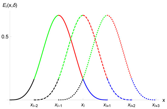
Figure 1. Plot of the extended cubic B-spline (ECBS) function.

For a function $\mathsf{\Psi }(x,t)$ there is a unique $\widehat{\mathsf{\Psi }}(x,t)$, that assures the prescribed conditions, such that

$$\widehat{\mathsf{\Psi }}(x,t)=\sum _{k=j-1}^{j+1}{C}_k^m\left(t\right)E_k(x,\delta ),$$

(6)

where time based undetermined coefficients $C_j\left(t\right)$’s are executed by such unique constraints. The relations (5) and (6) yield the following equations

$$\widehat{\mathsf{\Psi }}(x,t)=\sum _{k=j-1}^{j+1}{C}_k\left(t\right)E_k(x,\delta )=\left(\frac{4-\delta }{24}\right)C_{j-1}+\left(\frac{8+\delta }{12}\right)C_j+\left(\frac{4-\delta }{24}\right)C_{j+1}$$

(7)

$${\widehat{\mathsf{\Psi }}}^{\prime }(x,t)=\sum _{k=j-1}^{j+1}{C}_k\left(t\right)E_k^{\prime }(x,\delta )=\left(-\frac{1}{2h}\right)C_{j-1}+\left(\frac{1}{2h}\right)C_{j+1}$$

(8)

$${\widehat{\mathsf{\Psi }}}^{\prime \prime }(x,t)=\sum _{k=j-1}^{j+1}{C}_k\left(t\right)E_k^{\prime \prime }(x,\delta )=\left(\frac{2+\delta }{2h^2}\right)C_{j-1}+\left(-\frac{4+2\delta }{2h^2}\right)C_j+\left(\frac{2+\delta }{2h^2}\right)C_{j+1}.$$

(9)

3. Finite Difference Approximation for CFFD

In this part, we consider CFFD for the discretization in time dimension. Suppose $t_m=t_0+m\tau ,m=0,1,...,M$ in which $\tau =\frac{T}{M}$ is the step length in time direction. The FDM is employed for the discretization of CFFD. Using the Equation (4), CFFD can be described as:

$$\begin{array}{ccc}\hfill \frac{\partial {\mathsf{\Psi }}^{\nu }(x,t_{m+1})}{\partial t^{\nu }}& =& \frac{1}{1-\nu }{\int }_0^{t_{m+1}}\frac{\partial \mathsf{\Psi }(x,\eta )}{\partial \eta }exp[-\frac{\nu }{1-\nu }(t_{m+1}-\eta )]d\eta \hfill \\ & =& \frac{1}{1-\nu }\sum _{p=0}^m{\int }_{t_m}^{t_{m+1}}\frac{\partial \mathsf{\Psi }(x,\eta )}{\partial \eta }exp[-\frac{\nu }{1-\nu }(t_{m+1}-\eta )]d\eta \hfill \\ & =& \frac{1}{1-\nu }\sum _{p=0}^m[\frac{\mathsf{\Psi }(x,t_{p+1})-\mathsf{\Psi }(x,t_p)}{\tau }+O\left(\tau \right)]{\int }_{t_m}^{t_{m+1}}exp[-\frac{\nu }{1-\nu }(t_{m+1}-\eta )]d\eta \hfill \\ & =& \frac{1}{\tau (1-\nu )}\sum _{p=0}^m[\mathsf{\Psi }(x,t_{p+1})-\mathsf{\Psi }(x,t_p)]{\left[\frac{exp[-\frac{\nu }{1-\nu }(t_{m+1}-\eta )]}{\frac{\nu }{1-\nu }}\right]}_{t_p}^{t_{p+1}}+R_{\tau }^{\nu }\hfill \end{array}$$

For $m=0$, the above equation becomes

$$\frac{\partial {\mathsf{\Psi }}^{\nu }(x,t_{m+1})}{\partial t^{\nu }}\approx \frac{1}{\tau \nu }[\mathsf{\Psi }(x,t_1)-\mathsf{\Psi }(x,t_0)]\left(1-exp[-\frac{\nu }{1-\nu }\tau ]\right)exp[-\frac{\nu }{1-\nu }\tau ]$$

For $m=1$, we obtain

$$\begin{array}{cc}\hfill \frac{\partial {\mathsf{\Psi }}^{\nu }(x,t_{m+1})}{\partial t^{\nu }}\approx \frac{1}{\tau \nu }[\mathsf{\Psi }(x,t_1)-\mathsf{\Psi }(x,t_0& )]\left(1-exp[-\frac{\nu }{1-\nu }\tau ]\right)exp[-\frac{\nu }{1-\nu }2\tau ]\hfill \\ \hfill +& \frac{1}{\tau \nu }[\mathsf{\Psi }(x,t_2)-\mathsf{\Psi }(x,t_1)]\left(1-exp[-\frac{\nu }{1-\nu }\tau ]\right)exp[-\frac{\nu }{1-\nu }\tau ]\hfill \end{array}$$

The generalized form can be written as

$$\frac{\partial {\mathsf{\Psi }}^{\nu }(x,t_{m+1})}{\partial t^{\nu }}=\frac{1}{\tau \nu }\sum _{p=0}^m{\omega }_p[\mathsf{\Psi }(x,t_{m-p+1})-\mathsf{\Psi }(x,t_{m-p})]\left(1-exp[-\frac{\nu }{1-\nu }\tau ]\right)+R_{\tau }^{\nu },$$

(10)

where ${\omega }_p=exp[-\frac{\nu }{1-\nu }\tau p]$, The characteristics of ${\omega }_p$ coefficients can be easily proved:

• ${\omega }_0=1$
• ${\omega }_0>{\omega }_1>{\omega }_2>\dots >{\omega }_p$, ${\omega }_p\to 0$ as $p\to \infty$
• ${\omega }_p>0$ for $p=0,1,\dots ,m$
• ${\sum }_{p=0}^m({\omega }_p-{\omega }_{p+1})+{\omega }_{p+1}=(1-{\omega }_1)+{\sum }_{p=1}^{m-1}({\omega }_p-{\omega }_{p+1})+{\omega }_m=1$.

Remark 1.

The graphical results of ${\omega }_p=exp[-\frac{\nu }{1-\nu }\tau p]$ shows the asymptotic behaviour.

Theorem 1.

Suppose $\mathsf{\Psi }\left(x\right)$ be a function satisfies $C^2[a,b]$ and the fractional derivative $0<\nu <1$. Then the CFFD at knot $t_{m+1}$ is

$$\frac{\partial {\mathsf{\Psi }}^{\nu }(x,t_{m+1})}{\partial t^{\nu }}=\frac{1}{\tau \nu }\sum _{p=0}^m{\omega }_p[\mathsf{\Psi }(x,t_{m-p+1})-\mathsf{\Psi }(x,t_{m-p})]\left(1-exp[-\frac{\nu }{1-\nu }\tau ]\right)+O\left({\tau }^2\right).$$

(11)

Proof. 

From (10), we have

$$\begin{array}{ccc}\hfill R_{\tau }^{\nu }& =& \frac{1}{1-\nu }\sum _{p=0}^m{\int }_{t_m}^{t_{m+1}}exp[-\frac{\nu }{1-\nu }(t_{m+1}-\eta )]O\left(\tau \right)d\eta \hfill \\ & =& \frac{1}{1-\nu }\sum _{p=0}^m{\left[\frac{exp[-\frac{\nu }{1-\nu }(t_{m+1}-\eta )]}{\frac{\nu }{1-\nu }}\right]}_{t_p}^{t_{p+1}}O\left(\tau \right)\hfill \\ & =& \frac{1}{\nu }\sum _{p=0}^m\left[exp[-\frac{\nu }{1-\nu }(m-p)\tau ]-exp[-\frac{\nu }{1-\nu }(m-p+1)\tau ]\right]O\left(\tau \right)\hfill \end{array}$$

By expanding, we have

$$R_{\tau }^{\nu }=1-exp[-\frac{\nu }{1-\nu }(m+1)\tau ]O\left(\tau \right).$$

(12)

From the Taylor series of exponential function, we obtain

$$R_{\tau }^{\nu }\approx \left(\frac{\nu }{1-\nu }\right)(m+1)\tau O\left(\tau \right).$$

Therefore, we obtained the desired result

$$\frac{\partial {\mathsf{\Psi }}^{\nu }(x,t_{m+1})}{\partial t^{\nu }}=\frac{1}{\tau \nu }\sum _{p=0}^m{\omega }_p[\mathsf{\Psi }(x,t_{m-p+1})-\mathsf{\Psi }(x,t_{m-p})]\left(1-exp[-\frac{\nu }{1-\nu }\tau ]\right)+O\left({\tau }^2\right).$$

 □

4. Illustration of the Method

In this portion, we employ the CFFD and the ECBS to establish the numerical approach for solving TFRD equation. Using relations (6) and (10) in Equation (1), we obtain

$$\frac{1}{\tau \nu }\sum _{p=0}^m{\omega }_p[\widehat{\mathsf{\Psi }}(x_i,t_{m-p+1})-\widehat{\mathsf{\Psi }}(x_i,t_{m-p})]\left(1-exp[-\frac{\nu }{1-\nu }\tau ]\right)-d\frac{{\partial }^2\widehat{\mathsf{\Psi }}(x_i,t_{m+1})}{\partial x^2}+\alpha \widehat{\mathsf{\Psi }}(x_i,t_{m+1})=G(x_i,t_{m+1}).$$

(13)

Rearranging Equation (13), we have

$$\begin{array}{c}\frac{{\alpha }_1}{\tau \nu }\widehat{\mathsf{\Psi }}(x_i,t_{m+1})-d{\widehat{\mathsf{\Psi }}}^{\prime \prime }(x_i,t_{m+1})+\alpha \widehat{\mathsf{\Psi }}(x_i,t_{m+1})=\frac{{\alpha }_1}{\tau \nu }\widehat{\mathsf{\Psi }}(x_i,t_m)-\frac{{\alpha }_1}{\tau \nu }\sum _{p=1}^m{\omega }_p[\widehat{\mathsf{\Psi }}(x_i,t_{m-p+1})-\widehat{\mathsf{\Psi }}(x_i,t_{m-p})]\hfill \\ \hfill +G(x_i,t_{m+1}).\end{array}$$

The aforementioned equation can be written as

$$\begin{array}{c}\frac{{\alpha }_1}{\tau \nu }\sum _{k=j-1}^{j+1}{C}_k^{m+1}{E}_k-d\sum _{k=j-1}^{j+1}{C}_k^{m+1}{E}_k^{\prime \prime }+\alpha \sum _{k=j-1}^{j+1}{C}_k^{m+1}{E}_k=\frac{{\alpha }_1}{\tau \nu }\sum _{k=j-1}^{j+1}{C}_k^0{E}_k\hfill \\ \hfill +\frac{{\alpha }_1}{\tau \nu }\sum _{p=1}^m[{\omega }_p-{\omega }_{p+1}]\sum _{k=j-1}^{j+1}{C}_k^{m-p}{E}_k+G_k^{m+1}.\end{array}$$

(14)

The Equation (14) can be expressed in matrix form as

$$A{C}^{m+1}=B\left(C^0+\frac{{\alpha }_1}{\tau \nu }\sum _{p=1}^m[{\omega }_p-{\omega }_{p+1}]C^{m-p}\right)+H$$

(15)

where

$$A=\left[\begin{array}{ccccccc}{q}_1& q_2& q_1& 0& \dots & \dots & 0\\ 0& q_1& q_2& q_1& \dots & \dots & 0\\ ⋮& \dots & \ddots & \ddots & \ddots & \dots & ⋮\\ ⋮& \dots & \dots & q_1& q_2& q_1& 0\\ 0& \dots & \dots & \dots & q_1& q_2& q_1\end{array}\right]$$

(16)

$$B=\left[\begin{array}{ccccccc}{r}_1& r_2& r_1& 0& \dots & \dots & 0\\ 0& r_1& r_2& r_1& \dots & \dots & 0\\ ⋮& \dots & \ddots & \ddots & \ddots & \dots & ⋮\\ ⋮& \dots & \dots & r_1& r_2& r_1& 0\\ 0& \dots & \dots & \dots & r_1& r_2& r_1\end{array}\right]$$

(17)

$r_1=\frac{4-\delta }{24}$, $r_2=\frac{8+\delta }{12}$, $r_3=\frac{1}{2h}$, $r_4=\frac{2+\delta }{2h^2}$, $r_4=-\frac{2+\delta }{h^2}$, $q_1=\left(\frac{{\alpha }_1}{\tau \nu }+\alpha \right)r_1-d{r}_4$, $q_2=\left(\frac{{\alpha }_1}{\tau \nu }+\alpha \right)r_2-d{r}_5$ and $H={[G_0^{m+1},G_1^{m+1},...,G_{N+1}^{m+1}]}^T$. The above matrix system has of order $(N+1)\times (N+1)$. Two linear equations from the boundary conditions are necessary for a unique solution. To commence the iteration on the system, obtaining the initial vector is mandatory and we will use following initial conditions for the initial vector:

$$\left\{\begin{array}{c}{\widehat{\mathsf{\Psi }}}_0^{\prime }=\mathsf{\Psi }\left(x_0\right),\hfill \\ {\widehat{\mathsf{\Psi }}}_k^0=\mathsf{\Psi }\left(x_k\right),k=0,1,2,...,N\hfill \\ {\widehat{\mathsf{\Psi }}}_N^{\prime }=\mathsf{\Psi }\left(x_N\right).\hfill \end{array}\right.$$

(18)

5. Stability Analysis

The principle of stability is connected to computing method errors which do not rise as the procedure continues. We will analyze the stability using the Von Neumann approach. Suppose ${\xi }^m$ in the form of Fourier mode represents the growth factor and ${\widehat{\xi }}^m$ is the computed solution. Consequently, we defined the error term at mth time stage as

$${\mathsf{\Phi }}^m={\xi }^m-{\widehat{\xi }}^m.$$

(19)

Substituting Equation (19) in (14), we have obtained the error equation as follows:

$$\frac{{\alpha }_1}{\tau \nu }{\mathsf{\Phi }}^{m+1}-d{\mathsf{\Phi }}_{xx}^{m+1}+\alpha {\mathsf{\Phi }}^{m+1}=\frac{{\alpha }_1}{\tau \nu }{\mathsf{\Phi }}^0+\frac{{\alpha }_1}{\tau \nu }\sum _{p=1}^m[{\omega }_p-{\omega }_{p+1}]{\mathsf{\Phi }}^{m-p}.$$

(20)

Assume that the difference equation for the ECBS function in one Fourier mode as

$${\mathsf{\Phi }}_k^m={\lambda }^m{e}^{i\gamma hk},$$

(21)

where $h.\lambda ,\gamma$ and $i=\sqrt{-1}$ are the size of the element, Fourier coefficient, mode number respectively. Using the Equation (21) and ECBS functions in (20), we obtain

$$\begin{array}{c}\left[\left(\frac{{\alpha }_1}{\tau \nu }+\alpha \right)(r_1{e}^{i\gamma h(k-1)}+r_2{e}^{i\gamma hk}+r_1{e}^{i\gamma h(k+1)})-d(r_4{e}^{i\gamma h(k-1)}+r_5{e}^{i\gamma hk}+r_4{e}^{i\gamma h(k+1)})\right]{\lambda }^{m+1}\hfill \\ \hfill =\frac{{\alpha }_1}{\tau \nu }(r_1{e}^{i\gamma h(k-1)}+r_2{e}^{i\gamma hk}+r_1{e}^{i\gamma h(k+1)}){\lambda }^0+\frac{{\alpha }_1}{\tau \nu }\sum _{p=1}^m[{\omega }_p-{\omega }_{p+1}](r_1{e}^{i\gamma h(k-1)}+r_2{e}^{i\gamma hk}+r_1{e}^{i\gamma h(k+1)}){\lambda }^{m-p}.\end{array}$$

All throughout divided by $e^{i\gamma hk}$ and reorganization of the terms, we achieve

$$\begin{array}{c}\left[\left(\frac{{\alpha }_1}{\tau \nu }+\alpha \right)(r_2+2r_{1}cos\left(\gamma h\right))-d(r_5+2r_{4}cos\left(\gamma h\right))\right]{\lambda }^{m+1}=\frac{{\alpha }_1}{\tau \nu }(r_2+2r_{1}cos\left(\gamma h\right)){\lambda }^0+\hfill \\ \hfill \frac{{\alpha }_1}{\tau \nu }\sum _{p=1}^m[{\omega }_p-{\omega }_{p+1}](r_2+2r_{1}cos\left(\gamma h\right)){\lambda }^{m-p},\end{array}$$

Taking the term common on both sides then dividing by $r_2+2r_{1}cos\left(\gamma h\right)$, we attain

$$\left[\left(\frac{{\alpha }_1}{\tau \nu }+\alpha \right)+d\mu \right]{\lambda }^{m+1}=\frac{{\alpha }_1}{\tau \nu }{\lambda }^0+\frac{{\alpha }_1}{\tau \nu }\sum _{p=1}^m[{\omega }_p-{\omega }_{p+1}]{\lambda }^{m-p},$$

(22)

where $\mu =\frac{12\nu (2+\delta ){sin}^2\gamma h/2}{h^2(6+(\delta -4){sin}^2\gamma h/2)}>0$, $\delta \ne -2$.

Proposition 1.

Let ${\lambda }^m,m=0,1,\dots ,M$ be the solution of TFRD Equation (1), we have

$$|{\lambda }^m|\le |{\lambda }^0|,m=0,1,\dots ,M.$$

(23)

Proof. 

We verify this result with the assistance of mathematical induction. Substitute $m=0$ in Equation (22), we acquire

$$\left[\left(\frac{{\alpha }_1}{\tau \nu }+\alpha \right)+d\mu \right]{\lambda }^1=\frac{{\alpha }_1}{\tau \nu }{\lambda }^0.$$

Since $\frac{{\alpha }_1}{\tau \nu }+\alpha +d\mu >\frac{{\alpha }_1}{\tau \nu }$, we have

$$|{\lambda }^1|\le |{\lambda }^0|.$$

Assume that $|{\lambda }^m|\le |{\lambda }^0|$ for $m=0,1,\dots ,M-1.$ For $m+1$, we have

$$\begin{array}{ccc}\hfill \left[\left(\frac{{\alpha }_1}{\tau \nu }+\alpha \right)+d\mu \right]{\lambda }^{m+1}& =& \frac{{\alpha }_1}{\tau \nu }{\lambda }^0+\frac{{\alpha }_1}{\tau \nu }\sum _{p=1}^{m-1}[{\omega }_p-{\omega }_{p+1}]{\lambda }^{m-p}\hfill \\ \hfill \left[\left(\frac{{\alpha }_1}{\tau \nu }+\alpha \right)+d\mu \right]\left|{\lambda }^{m+1}\right|& \le & \frac{{\alpha }_1}{\tau \nu }|{\lambda }^0|+\frac{{\alpha }_1}{\tau \nu }\sum _{p=0}^{m-1}[{\omega }_p-{\omega }_{p+1}]\left|{\lambda }^{m-p}\right|\hfill \\ & =& \frac{{\alpha }_1}{\tau \nu }\left({\omega }_p+\sum _{p=0}^{m-1}[{\omega }_p-{\omega }_{p+1}]\right)\left|{\lambda }^0\right|\hfill \\ \hfill |{\lambda }^{m+1}|& \le & |{\lambda }^0|.\hfill \end{array}$$

Thus $|{\lambda }^{m+1}|=|{\mathsf{\Phi }}_k^{m+1}|\le |{\lambda }^0|=|{\mathsf{\Phi }}_k^0|$, so that $\parallel {\mathsf{\Phi }}_k^{m+1}{\parallel }_2\le {\parallel {\lambda }^0\parallel }_2.$ This implies that the proposed method for TFRD model is unconditionally stable. □

6. Convergence Analysis

First we recall some important findings to explain the convergence analysis.

Theorem 2

([42,43]). Notice that $\mathsf{\Psi }(x,t)\in C^4[a,b]$, $G\in C^2[a,b]$ and $[a,b]$ is subdivided at the equidistant knots with step length h. If $\tilde{\mathsf{\Psi }}(x,t)$ is the ECBS approximation for solving TRFD model at knots $x_0,...,x_N\in [a,b]$, then there are ${\sigma }_k$ free of h, such that

$$\parallel D^k(\mathsf{\Psi }(x,t)-\tilde{\mathsf{\Psi }}(x,t)){\parallel }_{\infty }\le {\sigma }_k{h}^{4-k},k=0,1,2$$

(24)

Lemma 1

([31,44]). The ECBS functions set $\{E_{-1},E_0,...,E_{N+1}\}$ explained in (5) acquires the result

$$\sum _{k=-1}^{N+1}\left|E_k(x,\delta )\right|\le \frac{7}{4},0\le x\le 1.$$

(25)

Theorem 3.

The $\widehat{\mathsf{\Psi }}(x,t)$ be the computational solution to the analytical $\mathsf{\Psi }(x,t)$ of the TFRD model. Furthermore, if $G\in C^2[0,1]$, we obtain

$$\begin{array}{c}\hfill \parallel \mathsf{\Psi }(x,t)-\widehat{\mathsf{\Psi }}{(x,t)\parallel }_{\infty }\le S{h}^2,t\ge 0,\end{array}$$

(26)

where constant $\sigma >0$ is a free of h and h is sufficiently small.

Proof. 

Assume that $\tilde{\mathsf{\Psi }}(x,t)={\sum }_{k=0}^N{\beta }_k{E}_k$ is the determined solution to the $\widehat{\mathsf{\Psi }}(x,t)$. Allow the present method for TFRD equation to achieve collocation condition as

$$L\mathsf{\Psi }(x_k,t)=L\widehat{\mathsf{\Psi }}(x_k,t)=G(x_k,t),k=0,\dots ,N$$

$$L\tilde{\mathsf{\Psi }}(x_k,t)=\tilde{G}(x_k,t),k=0,\dots ,N.$$

The difference equation of ECBS method for the TFRD model at mth time level, can be stated as

$$\begin{array}{c}\left(\frac{{\alpha }_1}{\tau \nu }+\alpha \right)(r_1{\mathsf{\Phi }}_{k-1}^{m+1}+r_2{\mathsf{\Phi }}_k^{m+1}+r_1{\mathsf{\Phi }}_{k+1}^{m+1})-d(r_4{\mathsf{\Phi }}_{k-1}^{m+1}+r_5{\mathsf{\Phi }}_k^{m+1}+r_4{\mathsf{\Phi }}_{k+1}^{m+1})\hfill \\ =\frac{{\alpha }_1}{\tau \nu }(r_1{\mathsf{\Phi }}_{k-1}^m+r_2{\mathsf{\Phi }}_k^m+r_1{\mathsf{\Phi }}_{k+1}^m)-\frac{{\alpha }_1}{\tau \nu }\sum _{p=1}^m{\omega }_p[r_1({\mathsf{\Phi }}_{k-1}^{m-p+1}-{\mathsf{\Phi }}_{k-1}^{m-p+1})+r_2({\mathsf{\Phi }}_k^{m-p+1}-{\mathsf{\Phi }}_k^{m-p})\\ \hfill +r_1({\mathsf{\Phi }}_{k+1}^{m-p}-{\mathsf{\Phi }}_{k+1}^{m-p})]+G^{m+1},\end{array}$$

(27)

and the boundary conditions are mentioned below:

$$r_1{\mathsf{\Phi }}_{k-1}^{m+1}+r_2{\mathsf{\Phi }}_k^{m+1}+r_1{\mathsf{\Phi }}_{k+1}^{m+1}=0,k=0,N,$$

where

$${\mathsf{\Phi }}_k^m={\beta }_k^m-C_k^m,k=-1,0,\dots ,N+1.$$

From Theorem 2, it is clear that

$${\kappa }_k^m=h^2[G_k^m-{\tilde{G}}_k^m]\le \sigma h^4.$$

Define ${\kappa }^m=max\left\{\right|{\kappa }_k^m|;0\le k\le N\},$ $E_k^m=\left|{\mathsf{\Phi }}_k^m\right|$ and $E^m=max\left\{\right|E_k^m|;0\le k\le N\}.$ For $m=0$ in (27), we have

$$\begin{array}{c}\left(\frac{{\alpha }_1}{\tau \nu }+\alpha \right)(r_1{\mathsf{\Phi }}_{k-1}^1+r_2{\mathsf{\Phi }}_k^1+r_1{\mathsf{\Phi }}_{k+1}^1)-d(r_4{\mathsf{\Phi }}_{k-1}^1+r_5{\mathsf{\Phi }}_k^1+r_4{\mathsf{\Phi }}_{k+1}^1)\hfill \\ \hfill =\frac{{\alpha }_1}{\tau \nu }(r_1{\mathsf{\Phi }}_{k-1}^0+r_2{\mathsf{\Phi }}_k^0+r_1{\mathsf{\Phi }}_{k+1}^0)+G^1.\end{array}$$

This implies

$$\left[\left(\frac{{\alpha }_1}{\tau \nu }+\alpha \right)r_2-d{r}_5\right]{\mathsf{\Phi }}_k^1=\left[\left(\frac{{\alpha }_1}{\tau \nu }+\alpha \right)r_1-d{r}_4\right]({\mathsf{\Phi }}_{k-1}^1-{\mathsf{\Phi }}_{k+1}^1)+G^1.$$

Take absolute values of ${\kappa }_k^1$, ${\mathsf{\Phi }}_k^1$ and from the initial condition $E^0=0$, we obtain

$$E_k^1\le \frac{6\sigma h^4}{(2+\delta )[(\frac{{\alpha }_1}{\tau \nu }+\alpha )h^2+12d]},k=0,1,\dots ,N$$

The following relations can be obtained from the boundary conditions:

$$E_{-1}^1\le \frac{(20+\delta )6\sigma h^4}{(4-\delta )(2+\delta )[(\frac{{\alpha }_1}{\tau \nu }+\alpha )h^2+12d]},$$

$$E_{N+1}^1\le \frac{(20+\delta )6\sigma h^4}{(4-\delta )(2+\delta )[(\frac{{\alpha }_1}{\tau \nu }+\alpha )h^2+12d]}.$$

Therefore

$$E^1\le {\sigma }_1{h}^2.$$

(28)

Here ${\sigma }_1$ is independent of h. Assume that $E^m\le {\sigma }_k{h}^2,$ for $k=1,\dots ,N$. Let $\sigma =max\{{\sigma }_k:0\le k\le N\},$ then from (27), we attain

$$\begin{array}{c}\left(\frac{{\alpha }_1}{\tau \nu }+\alpha \right)(r_1{\mathsf{\Phi }}_{k-1}^{m+1}+r_2{\mathsf{\Phi }}_k^{m+1}+r_1{\mathsf{\Phi }}_{k+1}^{m+1})-d(r_4{\mathsf{\Phi }}_{k-1}^{m+1}+r_5{\mathsf{\Phi }}_k^{m+1}+r_4{\mathsf{\Phi }}_{k+1}^{m+1})\hfill \\ \hfill ={\omega }_p\frac{{\alpha }_1}{\tau \nu }(r_1{\mathsf{\Phi }}_{k-1}^0+r_2{\mathsf{\Phi }}_k^0+r_1{\mathsf{\Phi }}_{k+1}^0)+\frac{{\alpha }_1}{\tau \nu }\sum _{p=0}^{m-1}[{\omega }_p-{\omega }_{p+1}](r_1{\mathsf{\Phi }}_{k-1}^{m-p}+r_2{\mathsf{\Phi }}_k^{m-p}+r_1{\mathsf{\Phi }}_{k+1}^{m-p})+G^{m+1}.\end{array}$$

Taking absolute values of ${\kappa }_k^m$, ${\mathsf{\Phi }}_k^m$, we obtain

$$E^{m+1}\le \frac{6\sigma h^2}{(2+\delta )[(\frac{{\alpha }_1}{\tau \nu }+\alpha )h^2+12d]}\left(\sum _{p=0}^{m-1}[{\omega }_p-{\omega }_{p+1}]\sigma h^2+\sigma h^2\right).$$

Similarly from the boundary conditions, we get

$$E_{-1}^{m+1}\le \sigma h^2,E_{N+1}^{m+1}\le \sigma h^2.$$

Hence, for every m, we have

$$E^{m+1}\le \sigma h^2.$$

(29)

From the above inequality and Theorem 1, we get

$$\tilde{\mathsf{\Psi }}(x,t)-\widehat{\mathsf{\Psi }}(x,t)=\sum _{k=-1}^{N+1}(C_k-{\beta }_k)E_k(x,\delta )\le \frac{7}{4}\sigma h^2.$$

(30)

By employing the triangular inequality, we have

$$\parallel \mathsf{\Psi }(x,t)-\widehat{\mathsf{\Psi }}{(x,t)\parallel }_{\infty }\le \parallel \mathsf{\Psi }(x,t)-\tilde{\mathsf{\Psi }}{(x,t)\parallel }_{\infty }+{\parallel \tilde{\mathsf{\Psi }}(x,t)-\widehat{\mathsf{\Psi }}(x,t)\parallel }_{\infty }.$$

By using inequalities (24) and (30), we obtain

$$\parallel \mathsf{\Psi }(x,t)-\widehat{\mathsf{\Psi }}{(x,t)\parallel }_{\infty }\le {\sigma }_0{h}^4+\frac{7}{4}\sigma h^2=S{h}^2,$$

where $S={\sigma }_0{h}^2+\frac{7}{4}$. Therefore, It can be deduced form Theorems 1 and 3:

$$\parallel \mathsf{\Psi }(x,t)-\widehat{\mathsf{\Psi }}{(x,t)\parallel }_{\infty }\le S{h}^2+O\left({\tau }^2\right).$$

 □

7. Illustration of Numerical Results

In this portion, we will go through some numerical results for the ECBS technique. The theoretical statements were verified with errors. All computational results can be carried out in any programming language. The errors between the results obtained by the ECBS and the analytical results $E_{\infty }(h,\tau )$ and $E_2(h,\tau )$ are estimated as

$$\begin{array}{c}\hfill E_{\infty }(h,\tau )=\underset{0\le m\le M}{max}{\parallel \mathsf{\Psi }(x,t_m)-\widehat{\mathsf{\Psi }}(x,t_m)\parallel }_{\infty },\end{array}$$

$$\begin{array}{c}\hfill E_2(h,\tau )=\sqrt{\sum _{m=0}^M{|\mathsf{\Psi }(x,t_m)-\widehat{\mathsf{\Psi }}(x,t_m)|}^2},\end{array}$$

The following definition can be employed numerically evaluate the convergence order:

$$Order=\frac{log\left(E_{\infty }\left(N_k\right)\right)-log\left(E_{\infty }\left(N_{k+1}\right)\right)}{log\left(2\right)},$$

where $E_{\infty }\left(N_k\right)$ and $E_{\infty }\left(N_{k+1}\right)$ are the errors at nodal points $N_k$ and $N_{k+1}$.

Example 1.

Consider the TFRD of the form:

$$\frac{{\partial }^{\nu }\mathsf{\Psi }(x,t)}{\partial t^{\nu }}=\frac{{\partial }^2\mathsf{\Psi }(x,t)}{\partial x^2}-\mathsf{\Psi }(x,t)+G(x,t),$$

with

$$\left\{\begin{array}{c}\mathsf{\Psi }(x,0)=0,0\le x\le 1\hfill \\ \mathsf{\Psi }(0,t)=\mathsf{\Psi }(1,t)=t^2,t\ge 0.\hfill \end{array}\right.$$

where $G(x,t)=\frac{2(1-x)sin\left(x\right)}{\nu }\left(t-\frac{1-\nu }{\nu }(1-e^{-\frac{\nu t}{1-\nu }})\right)+2t^2[cos\left(x\right)+(1-x)sin\left(x\right)]$ and analytical solution is $\mathsf{\Psi }(x,t)=t^2(1-x)sin\left(x\right)$ [11].

Table 1 shows the comparison of computational and analytical values corresponding to various $\nu$, $N=100$ and $\tau =0.005$ at $t=\frac{1}{2}$. Table 2 displays the maximum errors and the order of convergence for $\nu =0.7$, $N=40$ and $\tau =0.01$, $\nu =0.5$ respectively corresponding to numerous $\tau$ and h at $T=1$. Table 3 displays the $E_{\infty }$ and $E_2$ errors at $t=0.5,t=0.75$ and $T=1$ corresponding $\nu =0.5$. The piece-wise solutions of Example 1 for $N=100$, $\nu =0.4$, $\tau =0.0025$ at $T=1$ are shown in Equation (31). The polynomial also shows that the solution based on the basis function of degree 4. Figure 2 and Figure 3 depict the graphs of computational outcomes at dissimilar time sizes and errors at different $\tau$ corresponding $\nu =0.6$. Figure 4 illustrates the space–time plot for $\nu =0.7$, $N=80$ and $\tau =0.006$ at $T=0.6$. The graphical and computational results show that as we increase the number of partitioning in time–space directions, errors decrease.

Table 1. The computational and exact values for $N=100$ at $T=0.5$.

x	$\mathit{\nu }=0.2$	$\mathit{\nu }=0.4$	$\mathit{\nu }=0.6$	$\mathit{\nu }=0.8$	Exact Values
1/20	0.0118787	0.0118701	0.0119612	0.0123015	0.0118701
1/10	0.0224750	0.0225208	0.0225932	0.0230770	0.0224625
3/20	0.0317683	0.0317556	0.0318879	0.0323731	0.0317556
1/5	0.0397443	0.0397971	0.0398415	0.0402323	0.0397339
1/4	0.0463949	.04638820	0.0464550	0.0466942	0.0463882
3/10	0.0517182	0.0517589	0.0517344	0.0517962	0.0517160
7/20	0.0557184	0.0557209	0.0556901	0.0555741	0.0557209
2/5	0.0584061	0.0584300	0.0583377	0.0580631	0.0584128
9/20	0.0597977	0.0598078	0.0596973	0.0592977	0.0598078
1/2	0.0599159	0.0599272	0.0597940	0.0593122	0.0599282
11/20	0.0587890	0.0584305	0.0586576	0.0581412	0.0588023
3/5	0.0564511	0.0564582	0.0563224	0.0558194	0.0564642
13/20	0.0529421	0.0521149	0.0528272	0.0523818	0.0529538
7/10	0.0483069	0.0483176	0.0482151	0.0478636	0.0483163
3/4	0.0425960	0.0413353	0.0425333	0.0422999	0.0426024
4/5	0.0358646	0.0358818	0.0358333	0.0357260	0.0358678
17/20	0.0281728	0.0265245	0.0281699	0.0281761	0.0281730
9/10	0.0195849	0.0196028	0.0196016	0.0196841	0.0195832
19/20	0.0101698	0.0101677	0.0101901	0.0102820	0.0101677

Table 2. The maximum errors and order for $\nu =0.7$, $\nu =0.5$ corresponding $\tau$ and h.

$\mathit{\tau }$	${\mathit{E}}_{\mathit{\infty }}$	Order	h	${\mathit{E}}_{\mathit{\infty }}$	Order
$\frac{1}{04}$	0.074687677	…	$\frac{1}{05}$	0.072071696	…
$\frac{1}{08}$	0.018954332	1.97834	$\frac{1}{10}$	0.017726792	2.02350
$\frac{1}{16}$	0.004814144	1.97718	$\frac{1}{20}$	0.004285629	2.04835
$\frac{1}{32}$	0.001217257	1.98365	$\frac{1}{40}$	0.001014881	2.07820

Table 3. $E_{\infty }$ and $E_2$ for $\nu =0.5$ at various time.

$\mathit{\tau }$	h	t = 0.5		t = 0.75		T = 1
		${\mathit{E}}_{\infty }$	${\mathit{E}}_{\mathbf{2}}$	${\mathit{E}}_{\infty }$	${\mathit{E}}_{\mathbf{2}}$	${\mathit{E}}_{\infty }$	${\mathit{E}}_{\mathbf{2}}$
$\frac{1}{100}$	$\frac{1}{100}$	0.00908570	0.00066339	0.03367750	0.00245002	0.06323520	0.00459440
$\frac{1}{120}$	$\frac{1}{120}$	0.00560141	0.00037391	0.02026130	0.00134459	0.02563710	0.00169206
$\frac{1}{140}$	$\frac{1}{140}$	0.00160497	0.00009994	0.00761617	0.00046534	0.00930715	0.00055838
$\frac{1}{160}$	$\frac{1}{160}$	0.00084653	0.00004973	0.00276616	0.00015524	0.00484970	0.00026462
$\frac{1}{180}$	$\frac{1}{180}$	0.00029563	0.00001679	0.00044591	0.00002321	0.00067543	0.00002429

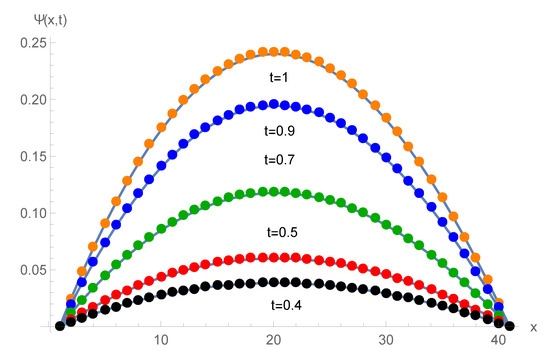
Figure 2. Numerical solution corresponding to time at $\nu =0.7$.

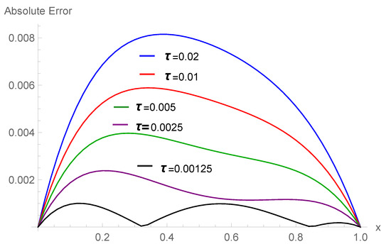
Figure 3. Error plot corresponding to $\tau$ for $\nu =0.8$, $N=100$ at $t=0.5$.

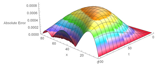
Figure 4. Space–time plot of errors corresponding $\nu =0.3$, $N=80$.

The piece-wise solution can be attained as:

$$\widehat{\mathsf{\Psi }}(x,t)=C_{j-1}^m{E}_{j-1}(x,\delta )+C_j^m{E}_j(x,\delta )+C_{j+1}^m{E}_{j+1}(x,\delta )$$

(31)

$$\widehat{\mathsf{\Psi }}(x,t)=\left\{\begin{array}{c}-1.94072\times {10}^{-16}+1.00666x-x^2\hfill \\ -6.73094x^3+331.117x^4,\hfill & x\in [\frac{0}{100},\frac{01}{100}),\hfill \\ 0.0000132708+1.00268x-0.601559x^2\hfill \\ -20.0333x^3+332.168x^4,\hfill & x\in [\frac{01}{100},\frac{02}{100}),\hfill \\ 0.000119841+0.986686x+0.198911x^2\hfill \\ -33.4144x^3+333.165x^4,\hfill & x\in [\frac{02}{100},\frac{03}{100}),\hfill \\ 0.000480787+0.950566x+1.40462x^2\hfill \\ -46.8677x^3+334.109x^4,\hfill & x\in [\frac{03}{100},\frac{04}{100}),\hfill \\ 0.00133918+0.886129x+3.01837x^2\hfill \\ -60.3869x^3+334.999x^4,\hfill & x\in [\frac{04}{100},\frac{05}{100}),\hfill \\ ⋮\hfill & ⋮\hfill \\ 16.3425-136.628x+433.632x^2\hfill \\ -610.188x^3+321.231x^4,\hfill & x\in [\frac{47}{100},\frac{48}{100}),\hfill \\ 17.6788-144.812x+449.979x^2\hfill \\ -620.079x^3+319.709x^4,\hfill & x\in [\frac{48}{100},\frac{49}{100}),\hfill \\ 19.0882-153.256x+466.455x^2\hfill \\ -629.744x^3+318.134x^4,\hfill & x\in [\frac{49}{100},\frac{50}{100}),\hfill \\ ⋮\hfill & ⋮\hfill \\ 162.168-678.223x+1065.79x^2\hfill \\ -744.798x^3+195.068x^4,\hfill & x\in [\frac{95}{100},\frac{96}{100}),\hfill \\ 165.943-686.831x+1068.11x^2\hfill \\ -738.684x^3+191.463x^4,\hfill & x\in [\frac{96}{100},\frac{97}{100}),\hfill \\ 169.645-694.963x+1069.65x^2\hfill \\ -732.161x^3+187.88x^4,\hfill & x\in [\frac{97}{100},\frac{98}{100}),\hfill \\ 173.264-702.59x+1070.39x^2\hfill \\ -725.228x^3+184.162x^4,\hfill & x\in [\frac{98}{100},\frac{99}{100}),\hfill \\ 176.787-709.682x+1070.31x^2\hfill \\ -717.885x^3+180.467x^4,\hfill & x\in [\frac{99}{100},\frac{100}{100}).\hfill \end{array}\right.$$

Example 2.

Consider the TFRD of the form:

$$\frac{{\partial }^{\nu }\mathsf{\Psi }(x,t)}{\partial t^{\nu }}=\frac{{\partial }^2\mathsf{\Psi }(x,t)}{\partial x^2}-\mathsf{\Psi }(x,t)+G(x,t),$$

with

$$\left\{\begin{array}{c}\mathsf{\Psi }(x,0)=0,0\le x\le 2\hfill \\ \mathsf{\Psi }(0,t)=\mathsf{\Psi }(2,t)=0,t\in [0,1].\hfill \end{array}\right.$$

where $G(x,t)=\frac{2x(2-x)}{\nu }\left(t-\frac{1-\nu }{\nu }(1-e^{-\frac{\nu t}{1-\nu }})\right)+t^2(2-x)x+2t^2$ and analytic solution is $\mathsf{\Psi }(x,t)=t^2(2-x)x$ [10,11].

Table 4 exhibits the maximum errors and order of convergence for $\nu =0.6$, different $\tau$ and h. Table 5 demonstrates that the comparison of computational and exact values corresponding different $\nu$, $N=100$ and $\tau =0.005$. Table 6 displays the $E_{\infty }$ and $E_2$ errors at $t=0.5,t=0.75$ and $T=1$ corresponding $\nu =0.5$. The computational values show that these results are compatible with the exact solutions. The piece-wise solutions of Example 2 for $N=100$, $\nu =0.4$, $\tau =0.002$ at $T=1$ are presented in Equation (32). This polynomial also presents that we have utilized the degree 4 basis function to obtain the computational outcomes. Figure 5 displays the numerical values at different time levels while Figure 6 and Figure 7 depict the comparison of errors for $\nu =0.5$ at $t=0.5$ and space–time graph of absolute errors for $\nu =0.4$, $N=100$ and $\tau =0.006$ at $t=\frac{06}{10}$.

Table 4. The errors and order for $\nu =0.6$ corresponding $\tau$ and h.

$\mathit{\tau }$	${\mathit{E}}_{\mathit{\infty }}$	Order	h	${\mathit{E}}_{\mathit{\infty }}$	Order
$\frac{1}{05}$	0.055515805	…	$\frac{1}{5}$	0.124485059	…
$\frac{1}{10}$	0.014037928	1.98357	$\frac{1}{10}$	0.030807675	2.01461
$\frac{1}{20}$	0.003540545	1.98729	$\frac{1}{20}$	0.007802263	1.98133
$\frac{1}{40}$	0.000850180	2.05813	$\frac{1}{40}$	0.001914559	2.02688

Table 5. The computational values and exact values of Example 2 corresponding $N=100$ at $T=1$.

x	$\mathit{\nu }=0.1$	$\mathit{\nu }=0.3$	$\mathit{\nu }=0.5$	$\mathit{\nu }=0.7$	Exact Values
0.1	0.190456	0.191839	0.196221	0.221592	0.19000
0.2	0.360661	0.362518	0.368566	0.401553	0.36000
0.3	0.510688	0.512392	0.518255	0.548109	0.51000
0.4	0.640598	0.641753	0.646276	0.667110	0.64000
0.5	0.750443	0.750840	0.753419	0.762705	0.75000
0.6	0.840262	0.839847	0.840307	0.837820	0.84000
0.7	0.910089	0.908924	0.907420	0.894491	0.91000
0.8	0.959948	0.958186	0.955114	0.934102	0.96000
0.9	0.989857	0.987712	0.983636	0.957540	0.99000
1.0	0.999826	0.997549	0.993127	0.965300	1.00000
1.1	0.989857	0.987712	0.983636	0.957540	0.99000
1.2	0.959948	0.958186	0.955114	0.934102	0.96000
1.3	0.910089	0.908924	0.907420	0.894491	0.91000
1.4	0.840262	0.839847	0.840307	0.837820	0.84000
1.5	0.750443	0.750840	0.753419	0.762705	0.75000
1.6	0.640598	0.641753	0.646276	0.667110	0.64000
1.7	0.510688	0.512392	0.518255	0.548109	0.51000
1.8	0.360661	0.362518	0.368566	0.401553	0.36000
1.9	0.190456	0.191839	0.196221	0.221592	0.19000

Table 6. $E_{\infty }$ and $E_2$ for $\nu =0.5$ at various time.

$\mathit{\tau }$	h	t = 0.5		t = 0.75		T = 1
		${\mathbf{E}}_{\infty }$	${\mathit{E}}_{\mathbf{2}}$	${\mathit{E}}_{\infty }$	${\mathit{E}}_{\mathbf{2}}$	${\mathit{E}}_{\infty }$	${\mathit{E}}_{\mathbf{2}}$
$\frac{1}{10}$	$\frac{1}{10}$	0.05497750	0.01286880	0.04825150	0.01101750	0.08207250	0.01848099
$\frac{1}{20}$	$\frac{1}{20}$	0.01783802	0.00288869	0.01149950	0.00244221	0.01925940	0.00249855
$\frac{1}{30}$	$\frac{1}{30}$	0.00778736	0.00097253	0.00853499	0.00125164	0.00977995	0.00107384
$\frac{1}{40}$	$\frac{1}{40}$	0.00357266	0.00034542	0.00554695	0.00058149	0.00807256	0.00087769
$\frac{1}{50}$	$\frac{1}{50}$	0.00106823	0.00009982	0.00335585	0.00033604	0.00673742	0.000677613

Figure 5. Numerical solution of Example 2 at $\nu =0.5$, $N=30$.

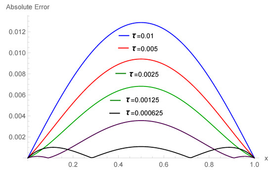
Figure 6. Absolute errors corresponding $\nu =0.5$, $N=100$ at $t=0.5$.

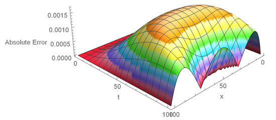
Figure 7. Space–time error plot for $\nu =0.4$, $N=100$ at $t=0.6$.

The piece-wise solution can be attained as:

$$\widehat{\mathsf{\Psi }}(x,t)=C_{j-1}^m{E}_{j-1}(x,\delta )+C_j^m{E}_j(x,\delta )+C_{j+1}^m{E}_{j+1}(x,\delta )$$

(32)

$$\widehat{\mathsf{\Psi }}(x,t)=\left\{\begin{array}{c}-8.67362\times {10}^{-18}+2.04601x-x^2\hfill \\ -14.201x^3+358.103x^4,\hfill & x\in [0,\frac{02}{100}),\hfill \\ 0.000227971+2.01183x+0.706653x^2\hfill \\ -42.541x^3+355.496x^4,\hfill & x\in [\frac{02}{100},\frac{04}{100}),\hfill \\ 0.00203554+1.87643x+4.08378x^2\hfill \\ -70.4828x^3+352.985x^4,\hfill & x\in [\frac{04}{100},\frac{06}{100}),\hfill \\ 0.0080838+1.57454x+9.09789x^2\hfill \\ -98.0488x^3+350.567x^4,\hfill & x\in [\frac{06}{100},\frac{08}{100}),\hfill \\ 0.022302+1.04254x+15.718x^2\hfill \\ -125.26x^3+348.238x^4,\hfill & x\in [\frac{08}{100},\frac{10}{100}),\hfill \\ ⋮\hfill & ⋮\hfill \\ 248.472-1044.27x+1651.08x^2\hfill \\ -1159.38x^3+305.1x^4,\hfill & x\in [\frac{94}{100},\frac{96}{100}),\hfill \\ 270.008-1111.5x+1720.99x^2\hfill \\ -1183.52x^3+305.032x^4,\hfill & x\in [\frac{96}{100},\frac{98}{100}),\hfill \\ 292.945-1181.69x+1792.54x^2\hfill \\ -1207.79x^3+304.998x^4,\hfill & x\in [\frac{98}{100},1.00),\hfill \\ ⋮\hfill & ⋮\hfill \\ 4634.71-9704.42x+7621.88x^2\hfill \\ -2660.65x^3-50.7798x^4,\hfill & x\in [\frac{190}{100},\frac{192}{100}),\hfill \\ 4864.23-10079.5x+7834.42x^2\hfill \\ -2706.49x^3+350.567x^4,\hfill & x\in [\frac{192}{100},\frac{194}{100}),\hfill \\ 5103.99-10467x+8052.84x^2\hfill \\ -2753.4x^3+352.985x^4,\hfill & x\in [\frac{194}{100},\frac{196}{100}),\hfill \\ 5354.46-10870.2x+8277.37x^2\hfill \\ -2801.43x^3+355.496x^4,\hfill & x\in [\frac{196}{100},\frac{198}{100}),\hfill \\ 5616.13-11286.9x+8508.26x^2\hfill \\ -2850.62x^3+358.103x^4,\hfill & x\in [\frac{198}{100},2.00).\hfill \end{array}\right.$$

8. Conclusions

A ECBS collocation approach for the solution of the TFRD model was reported in this research paper. ECBS was employed for space discretization while CFFD was applied for time direction. The CFFD operator is used for the first time in B-spline methods. The operator is successfully utilized for the ECBS method. This approach has order 2 accuracy in time and space dimensions. Thus, the ECBS method with a non-singular kernel leads to accurate computational results. A variety of computational examples have validated the ECBS collocation approach.

References

- Murray, J.D. Mathematical Biology; Springer: New York, NY, USA, 2003. [Google Scholar]
- Kuramoto, Y. Chemical Oscillations Waves and Turbulence; Dover Publications, Inc.: Mineola, NY, USA, 2003. [Google Scholar]
- Wilhelmsson, H.; Lazzaro, E. Reaction–Diffusion Problems in the Physics of hot Plasmas; Institute of Physics Publishing: Bristol, UK; Philadelphia, PA, USA, 2001. [Google Scholar]
- Hundsdorfer, W.; Verwer, J.G. Numerical Solution of Time Dependent Advection-Diffusion-Reaction Equations; Springer: Berlin, Germany, 2003. [Google Scholar]
- Bar, M.; Gottschalk, N.; Eiswirth, M.; Ertl, G. Spiral waves in a surface reaction: Model calculations. J. Chem. Phys. 1994, 100, 1202–1214. [Google Scholar] [CrossRef]
- Mainardi, F.; Raberto, M.; Gorenflo, R.; Scalas, R. Fractional calculus and continuous-time finance. II: The waiting-time distribution. Physica A 2000, 287, 468–481. [Google Scholar] [CrossRef]
- Benson, D.A.; Wheatcraft, S.; Meerschaert, M.M. Application of a fractional advection-dispersion equation. Water Resour. Res. 2000, 36, 1403–1412. [Google Scholar] [CrossRef]
- Metzler, R.; Klafter, J. The random walks guide to anomalous diffusion: A fractional dynamics approach. Phys. Rep. 2000, 339, 1–77. [Google Scholar] [CrossRef]
- Hafez, R.M.; Youssri, Y.H. Jacobi collocation scheme for variable-order fractional reaction sub-diffusion equation. Comput. Appl. Math. 2018, 37, 5315–5333. [Google Scholar] [CrossRef]
- Zhang, J.; Yang, X. A class of efficient difference method for time fractional reaction-diffusion equation. Comput. Appl. Math. 2018, 37, 4376–4396. [Google Scholar] [CrossRef]
- Kanth, A.S.V.R.; Garg, N. A numerical approach for a class of time-fractional reaction-diffusion equation through exponential B-spline method. Comput. Appl. Math. 2019, 39, 09–37. [Google Scholar] [CrossRef]
- Caputo, M.; Fabrizio, M. A new Definition of Fractional Derivative without Singular Kernel. Prog. Fract. Differ. Appl. 2015, 1, 73–85. [Google Scholar]
- Atangana, A.; Alkahtani, B.S.T. Extension of the resistance inductance, capacitance electrical circuit of fractional derivative without singular kernel. Adv. Mech. Eng. 2015, 7, 1–6. [Google Scholar] [CrossRef]
- Gómez-Aguilar, J.F.; L’opez-L’opez, M.G.; Alvarado-Mart’ınez, V.M.; Reyes-Reyes, J.; Adam-Medina, M. Modeling diffusive transport with a fractional derivative without singular kernel. Physica A 2016, 447, 467–481. [Google Scholar] [CrossRef]
- Gomez, J.F.; Martinez, H.Y.; Ramon, C.C.; Orduna, I.C.; Jimenez, R.F.E.; Peregrino, V.H.O. Modeling of a mass-spring-damper system by fractional derivative with and without a singular kernel. Entropy 2015, 17, 6289–6303. [Google Scholar] [CrossRef]
- Atangana, A. On the new fractional derivative and application to nonlinear Fisher’s reaction-diffusion equation. Appl. Math. Comput. 2016, 273, 948–956. [Google Scholar] [CrossRef]
- Yang, X.J.; Zhang, Z.Z.; Srivastava, H.M. Some new applications for heat and fluid flows via fractional derivatives without singular kernel. Therm. Sci. 2016, 20, 833–839. [Google Scholar] [CrossRef]
- Rida, S.Z.; El-sayed, A.M.A.; Arafa, A.A.M. On the solutions of time-fractional reaction-diffusion equations. Commun. Nonlinear Sci. Numer. Simul. 2010, 15, 3847–3854. [Google Scholar] [CrossRef]
- Turut, V.; Guzel, N. Comparing numerical methods for solving time-fractional reaction-diffusion equations. Math. Anal. 2012, 2012, 28p. [Google Scholar] [CrossRef]
- Gong, C.; Bao, W.M.; Tang, G.; Jiang, Y.W.; Liu, J. A domain decomposition method for time fractional reaction-diffusion equation. Sci. World J. 2014, 2014, 5p. [Google Scholar] [CrossRef]
- Sungu, I.C.; Demir, H. A new approach and solution technique to solve time fractional non-linear reaction-diffusion equation. Math. Prob. Eng. 2015, 2015, 13p. [Google Scholar]
- Liu, J.; Gong, C.; Bao, W.; Tang, G.; Jiang, Y. Solving the Caputo fractional reaction-diffusion equation on GPU. Discret. Dyn. Nat. Soc. 2014, 2014, 820162. [Google Scholar] [CrossRef]
- Liu, Y.; Du, Y.; Li, H.; Wang, J. An H1-Galerkin mixed finite element method for time fractional reaction-diffusion equation. J. Appl. Math. Comput. 2015, 47, 103–117. [Google Scholar] [CrossRef]
- Wang, Q.L.; Liu, J.; Gong, C.Y.; Tang, X.T.; Fu, G.T.; Xing, Z.C. An efficient parallel algorithm for Caputo fractional reaction-diffusion equation with implicit finite difference method. Adv. Differ. Equ. 2016, 1, 207–218. [Google Scholar] [CrossRef]
- Rashidinia, J.; Mohmedi, E. Convergence analysis of tau scheme for the fractional reaction-diffusion equation. Eur. Phys. J. Plus 2018, 133, 402. [Google Scholar] [CrossRef]
- Ersoy, O.; Dag, I. Numerical solutions of the reaction diffusion system by using exponential cubic B-spline collocation algorithms. Open Phys. 2015, 13, 414–4275. [Google Scholar] [CrossRef]
- Zheng, M.L.; Liu, F.W.; Liu, Q.X.; Burrage, K.; Simpson, M.J. Numerical solution of the time fractional reaction-diffusion equation with a moving boundary. J. Comput. Phys. 2017, 338, 493–510. [Google Scholar] [CrossRef]
- Owelabi, K.M.; Dutta, H. Numerical Solution of space-time fractional reaction-diffusion equations via the Caputo and Riesz derivatives. Math. Appl. Eng. Model Soc. Issues 2019, 39, 161–188. [Google Scholar]
- Zeynab, K.; Habibollah, S. B-spline wavelet operational method for numerical solution of time-space fractional partial differential equations. Int. J. Wavelets Multiresolut. Inf. Process. 2017, 15, 3401–3424. [Google Scholar]
- Pandey, P.; Kumar, S.; Gömez-Aguilar, J.F. Numerical Solution of the Time Fractional reaction-advection- diffusion Equation in Porous Media. J. Appl Comput. Mech. 2019, 7. [Google Scholar] [CrossRef]
- Akram, T.; Abbas, M.; Ismail, A.I. An extended cubic B-spline collocation scheme for time fractional sub-diffusion equation. AIP Conf. Proc. 2019, 2184, 060017. [Google Scholar]
- Akram, T.; Abbas, M.; Ismail, A.I. Numerical solution of fractional cable equation via extended cubic B-spline. AIP Conf. Proc. 2019, 2138, 030004. [Google Scholar]
- Akram, T.; Abbas, M.; Ismail, A.I.; Ali, N.M.; Baleanu, D. Extended cubic B-splines in the numerical solution of time fractional telegraph equation. Adv. Differ. Equ. 2019, 2019, 365. [Google Scholar] [CrossRef]
- Akram, T.; Abbas, M.; Iqbal, A.; Baleanu, D.; Asad, J.H. Novel Numerical Approach Based on Modified Extended Cubic B-Spline Functions for Solving Non-Linear Time-Fractional Telegraph Equation. Symmetry 2020, 12, 1154. [Google Scholar] [CrossRef]
- Akram, T.; Abbas, M.; Ali, A. A numerical study on time fractional Fisher equation using an extended cubic B-spline approximation. J. Math. Comput. Sci. 2021, 22, 85–96. [Google Scholar] [CrossRef]
- Akram, T.; Abbas, M.; Riaz, M.B.; Ismail, A.I.; Ali, N.M. An efficient numerical technique for solving time fractional Burgers equation. Alex Eng. J. 2020, 59, 2201–2220. [Google Scholar] [CrossRef]
- Akram, T.; Abbas, M.; Riaz, M.B.; Ismail, A.I.; Ali, N.M. Development and analysis of new approximation of extended cubic B-spline to the non-linear time fractional Klein-Gordon equation. Fractals 2020, in press. [Google Scholar] [CrossRef]
- Khalid, N.; Abbas, M.; Iqbal, M.K.; Baleanu, D. A numerical algorithm based on modified extended B-spline functions for solving time fractional diffusion wave equation involving reaction and damping terms. Adv. Differ. Equ. 2019, 2019, 378. [Google Scholar] [CrossRef]
- Khalid, N.; Abbas, M.; Iqbal, M.K.; Singh, J.; Ismail, A.I. A computational approach for solving time fractional differential equation via spline functions. Alex Eng. J. 2020, in press. [Google Scholar] [CrossRef]
- Losada, J.; Nieto, J.J. Properties of a New Fractional Derivative without Singular Kernel. Prog. Fract. Differ. Appl. 2015, 1, 87–92. [Google Scholar]
- Han, L.X.; Liu, S.J. An extension of the cubic uniform B-spline curves. Comput. Aided Des. Comput. Graph. 2003, 15, 576–578. [Google Scholar]
- Hall, C.A. On error bounds for spline interpolation. J. Approx. Theory 1968, 1, 209–218. [Google Scholar] [CrossRef]
- Boor, C.D. On the convergence of odd degree spline interpolation. J. Approx. Theory 1968, 1, 452–463. [Google Scholar] [CrossRef]
- Sharifi, S.; Rashidinia, J. Numerical solution of hyperbolic telegraph equation by cubic B-spline collocation method. Appl. Math. Comput. 2016, 281, 28–38. [Google Scholar] [CrossRef]
© 2020 by the authors. Licensee MDPI, Basel, Switzerland. This article is an open access article distributed under the terms and conditions of the Creative Commons Attribution (CC BY) license (http://creativecommons.org/licenses/by/4.0/).