Eigenvalue Based Approach for Assessment of Global Robustness of Nonlinear Dynamical Systems

Abstract

In this paper we have established the sufficient conditions for asymptotic convergence of all solutions of nonlinear dynamical system (with potentially unknown and unbounded external disturbances) to zero with time $t\to \infty .$ We showed here that the symmetric part of linear part of nonlinear nominal system, or, to be more precise, its time-dependent eigenvalues, play important role in assessment of the robustness of systems.

1. Notations, Motivation and Introduction

Our purpose here is to prove a new result regarding the convergence of all solutions to the origin $x=0$ as $t\to \infty$ for a nonlinear dynamical system subject to external disturbances,

$$\dot{x}=f(x,t)+\delta (x,t),x\in {\mathbb{R}}^n,t\ge t_0,$$

(1)

given that 0 is a solution for the nominal system $\dot{x}=f(x,t)$ and that f and $\delta$ satisfy certain conditions.

1.1. Notations

Let ${\mathbb{R}}^n$ denote n-dimensional vector space endowed by the Euclidean norm ${∥·∥}_2,$ and $∥·∥$ be an induced norm for matrices, $∥A∥=max\{{∥Ax∥}_2;{∥x∥}_2=1\}.$ We always assume that the function f is continuously differentiable, $f(0,t)=0$ for all $t\ge t_0,$ that perturbation $\delta$ is at least continuous both from ${\mathbb{R}}^n\times [t_0,\infty )$ to ${\mathbb{R}}^n,$ and it is not assumed that the zero function is a solution of (1). The nonlinear term $\delta (x,t)$ aggregates all external disturbances which affect the state variable $x\in {\mathbb{R}}^n$ of the nominal system $\dot{x}=f(x,t).$ Let us denote by $A(t)$ the linear part of nominal vector field $f(x,t)$ at $x=0,$ that is, $A(t)\triangleq J_{x}f(0,t),$ where $J_{x}f$ denotes the Jacobian matrix of f with respect to variable x and let us assume that $f(x,t)=A(t)x+R_1(x,t)$ for all $x\in {\mathbb{R}}^n$ and all $t\ge t_0,$ where $R_1$ is the Taylor remainder. We also assume that the solutions of (1) are uniquely determined by $x(t_0)$ for all $t\ge t_0.$ Throughout the whole paper, the superscript “T” indicates the transpose operator.

1.2. Motivation and Introduction

For a motivation, let us consider the case when linear part $\dot{x}=A(t)x$ of the nominal system $\dot{x}=f(x,t)$ is asymptotically stable. What can we say about the asymptotic behavior (as $t\to \infty$) of solutions of perturbed system (1)? This question represents one of the fundamental problems in the area of robust stability and robustness of the systems in general and so the effect of (known or unknown) perturbations on the solutions of nominal system as a potential source of instability attracts the attention and interest of scientific community for a long time in the various contexts, recently for example [1,2,3,4,5,6,7,8,9,10,11,12,13,14,15,16]. A comprehensive overview of the most significant results on robust control theory as a stand-alone subfield of control theory and its history is presented in [17,18].

On the other side, the analysis of the robustness of uncontrolled systems often merges with the mathematical theory of dynamical systems. As is traditional in perturbation theory of linear and nonlinear dynamical systems, the behavior of solutions of a perturbed system is determined in terms of the behavior of solutions of an unperturbed system [19,20,21,22,23]. In principle, to answer the question regarding behavior of the solutions of perturbed systems as $t\to \infty$, it usually makes a difference whether the origin remains an equilibrium for the perturbed system or not. If $\delta (0,t)=0$, then the origin is an equilibrium point of (1). In this case, we can analyze the stability property of the origin as an equilibrium point of the perturbed system. It is worth mentioning in this context the well-known Demidovich condition [24] on asymptotic stability of all solutions of a nonlinear system $\dot{x}=F(x,t)$ stating that if for some positive definite matrix $P=P^T>0,$ the matrix

$$J(x,t)=\frac{1}{2}\left[P{J}_{x}F(x,t)+J_x^{T}F(x,t)P\right]$$

(2)

is negative definite uniformly in $(x,t)\in {\mathbb{R}}^n\times \mathbb{R}$ then for any two solutions $x_1(t)$ and $x_2(t)$ is ${∥x_1(t)-x_2(t)∥}_2\le K\exp [-\alpha (t-t_0)]{∥x_1(t_0)-x_2(t_0)∥}_2$ for all $t\ge t_0$ and some independent on $x_1$ and $x_2$ constants $K,\alpha >0,$ but this condition is not-very-well suited for reasoning about the convergence of all solutions to zero as $t\to \infty$ if $F(0,t)\ne 0$ and so we can not set $x_2(t)\equiv 0.$ In this case, that is, if $\delta (0,t)\ne 0$, the origin is no longer an equilibrium point of (1), and we usually analyze the ultimate boundedness of solutions of perturbed system. As have been shown in ([25] Chapter 9), if the point $x=0$ is an exponentially stable equilibrium point of the nominal system and perturbation term $\delta$ satisfies

$${∥\delta (x,t)∥}_2\le \gamma (t){∥x∥}_2+\eta (t),{∥x∥}_2<r,t\ge t_0$$

(3)

where $\gamma ,\eta :[t_0,\infty )\to [0,\infty )$ are continuous, ${\int }_{t_0}^{\infty }\gamma (\tau )d\tau <\infty$ and $\eta$ is bounded, then for $\eta \equiv 0,$ the origin is an exponentially stable equilibrium point of the perturbed system and the solutions of the perturbed system are ultimately bounded in the opposite case (if $\eta$ is not identically zero). These analyses are close and compatible with the concept input-to-state stability which has been introduced by E. Sontag [26,27]. In contrast to the case of exponential stability, the unperturbed system with uniformly asymptotically stable (but not exponentially stable) zero solution is not robust even for continuous perturbations with arbitrarily small linear bounds ${∥\delta (x,t)∥}_2\le \gamma {∥x∥}_2,$ ${∥x∥}_2<r,$ $t\ge t_0$ and $\gamma >0,$ see [25] for more details. The definitions of various types of stability for non-autonomous systems mentioned here can be found, for example, in ([25] Chapter 4). There are two useful and principally different methods for studying the qualitative behavior of the solutions of the perturbed nonlinear system: the second method of Lyapunov [25,28,29,30], and the use of a variation of constants formula [19,20,21,31]. The present paper is based on the second approach in combination with the eigenvalue techniques to prove, in Theorem 1 with the help of Lemma 1, the new sufficient conditions for global robustness of nonlinear (uncontrolled) systems, whose linear part $\dot{x}=A(t)x$ is asymptotically stable and in general time-varying; the notion “global robustness” is meant in the sense of convergence of all solutions of system (1) to the origin $x=0$ as $t\to \infty$ provided the perturbing term satisfies some growth constraints. At this point, we would also like to emphasize that we achieve our results without a priori assumption on the boundedness of perturbation $\delta (x,t).$ More specifically, $\eta (t)$ in (3) may not be bounded for $\gamma (t)\equiv 0,$ and so our ambition here is to partially complement the mosaic of asymptotic behavior of the solutions of dynamical systems. The theory is illustrated by two nontrivial examples, Example 1 and Example 2.

2. Results

In this section, we formulate the main result on the asymptotic behavior of solutions for (1) as $t\to \infty .$

2.1. Auxiliary Lemma

The purpose of this subsection is to present the lemma upon which subsequent result will be based. The core part of the proof of the later result is contained in the proof of this lemma.

Lemma 1.

Let $X(t)$ be a fundamental matrix of $\dot{x}=A(t)x.$ Denote the largest and smallest pointwise eigenvalues of $\frac{1}{2}[A(t)+A^T(t)]$ by ${\lambda }_{max}(t)$ and ${\lambda }_{min}(t).$ Then

$$\exp \left[\underset{\tau }{\overset{t}{\int }}{\lambda }_{min}(s)ds\right]\le ∥X(t)X^{-1}(\tau )∥\le \exp \left[\underset{\tau }{\overset{t}{\int }}{\lambda }_{max}(s)ds\right],t\ge \tau \ge t_0.$$

(4)

Proof. 

First note that the integrals in (4) are well defined since the eigenvalues of a matrix are continuous functions of the entries of the matrix, and because the entries of $\frac{1}{2}[A(t)+A^T(t)]$ are continuous functions of time, the frozen-time eigenvalues ${\lambda }_{max}(t)$ and ${\lambda }_{min}(t)$ are also continuous functions of $t.$ Suppose $x(t)$ is a solution of $\dot{x}=A(t)x$ corresponding to a given $t_0$ and nonzero $x(t_0).$ Using

$$\frac{d}{dt}{∥x(t)∥}_2^2=\frac{d}{dt}[x^T(t)x(t)]=x^T(t)[A^T(t)+A(t)]x(t)$$

the Rayleigh–Ritz inequality [32] gives

$$2{∥x(t)∥}_2^2{\lambda }_{min}(t)\le \frac{d}{dt}{∥x(t)∥}_2^2\le 2{∥x(t)∥}_2^2{\lambda }_{max}(t),t\ge t_0.$$

Dividing through by ${∥x(t)∥}_2^2$ which is positive at each $t,$ and integrating from $\tau$ to any $t\ge \tau \ge t_0$ yields

$$2\underset{\tau }{\overset{t}{\int }}{\lambda }_{min}(s)ds\le \ln {∥x(t)∥}_2^2-\ln {∥x(\tau )∥}_2^2\le 2\underset{\tau }{\overset{t}{\int }}{\lambda }_{max}(s)ds,t\ge \tau \ge t_0.$$

Exponentiation followed by taking the nonnegative square root gives

$${∥x(\tau )∥}_2\exp \left[\underset{\tau }{\overset{t}{\int }}{\lambda }_{min}(s)ds\right]\le {∥x(t)∥}_2\le {∥x(\tau )∥}_2\exp \left[\underset{\tau }{\overset{t}{\int }}{\lambda }_{max}(s)ds\right],t\ge \tau \ge t_0.$$

(5)

Now, given any $\tau \ge t_0$ and ${\tau }^{*}\ge \tau$ let $x^{*}$ be such that

$${∥x^{*}∥}_2=1,{∥X({\tau }^{*})X^{-1}(\tau )x^{*}∥}_2=∥X({\tau }^{*})X^{-1}(\tau )∥.$$

Note that such $x^{*}$ exists from the definition of induced norm for matrices. Then the initial state $x(\tau )=x^{*}$ yields a solution of $\dot{x}=A(t)x$ that at time ${\tau }^{*}$ satisfies

$${∥x({\tau }^{*})∥}_2={∥X({\tau }^{*})X^{-1}(\tau )x^{*}∥}_2=∥X({\tau }^{*})X^{-1}(\tau )∥\le {∥x(\tau )∥}_2\exp \left[\underset{\tau }{\overset{{\tau }^{*}}{\int }}{\lambda }_{max}(s)ds\right].$$

In the last inequality, we used the right inequality from (5) for $t={\tau }^{*}$ and the fact that $x({\tau }^{*})=X({\tau }^{*})X^{-1}(\tau )x^{*}.$ Since $x(\tau )=x^{*}$ and ${∥x^{*}∥}_2=1,$ the last inequality gives that

$$∥X({\tau }^{*})X^{-1}(\tau )∥\le \exp \left[\underset{\tau }{\overset{{\tau }^{*}}{\int }}{\lambda }_{max}(s)ds\right].$$

Because such $x^{*}$ can be selected for any $\tau \ge t_0$ and ${\tau }^{*}\ge \tau ,$ the proof of the right inequality in (4) is complete. The other half of the theorem follows by analogous arguments. □

Taking into consideration the fact that linear system $\dot{x}=A(t)x$ is uniformly asymptotically stable if and only if $∥X(t)X^{-1}(\tau )∥\le K\exp [-\alpha (t-\tau )],$ $t_0\le \tau \le t<\infty$ for some positive constants K and $\alpha$ [33], we have the following

Corollary 1.

If ${\lambda }_{max}(t)\le {\lambda }_0<0$ for all $t\ge t_0,$ then the linear system $\dot{x}=A(t)x,$$t\ge t_0$ is uniformly asymptotically stable (⇔ uniformly exponentially stable).

2.2. Main Result

Theorem 1.

Let us consider the system (1), $\dot{x}=f(x,t)+\delta (x,t),x\in {\mathbb{R}}^n,t\ge t_0.$ Assume that

(A1) 

${\lambda }_{max}(t)\le {\lambda }_0<0$ in some left neighborhood of $+\infty ,$ where ${\lambda }_{max}(t)$ is the largest pointwise eigenvalue of $\frac{1}{2}[A(t)+A^T(t)],$ $A(t)=J_{x}f(0,t);$

(A2) 

for all $(x,t)\in {\mathbb{R}}^n\times [t_0,\infty )$ is ${∥\delta (x,t)∥}_2\le {∥\tilde{\mathsf{\Delta }}(t)∥}_2-{∥f(x,t)-[J_{x}f(0,t)]x∥}_2,$ where function $\tilde{\mathsf{\Delta }}(t)$ is continuous on $[t_0,\infty )$ and satisfies

(A3) 

$\underset{t\to \infty }{lim}\left({∥\tilde{\mathsf{\Delta }}(t)∥}_2/{\lambda }_{max}(t)\right)=0.$

Then all solutions of (1) converge to 0 as $t\to \infty .$

Proof. 

The effect of the perturbation on the solutions of a system of nonlinear differential equations can be studied using the variation of constants formula identifying the Taylor remainder of f together with $\delta$ as an inhomogeneous term $\mathsf{\Delta }(x,t).$ Thus we can rewrite the system (1) as

$$\dot{x}(t)=A(t)x(t)+\mathsf{\Delta }(x,t),$$

where $A(t)\triangleq J_{x}f(0,t)$ and $\mathsf{\Delta }(x,t)\triangleq R_1(x,t)+\delta (x,t).$ Then for all $t\ge t_0,$

$$x(t)=X(t)X^{-1}(t_0)x(t_0)+\underset{t_0}{\overset{t}{\int }}X(t)X^{-1}(\tau )\mathsf{\Delta }(x(\tau ),\tau )d\tau ,$$

(6)

where $X(t),$$t\ge t_0$ is a fundamental matrix of $\dot{x}=A(t)x$ representing the linear part of nominal system $\dot{x}=f(x,t).$ Thus

$${∥x(t)∥}_2\le ∥X(t)X^{-1}(t_0)∥{∥x(t_0)∥}_2+\underset{t_0}{\overset{t}{\int }}∥X(t)X^{-1}(\tau )∥{∥\mathsf{\Delta }(x(\tau ),\tau )∥}_{2}d\tau .$$

Since by Assumption A2 is ${∥\mathsf{\Delta }(x,t)∥}_2\le {∥\tilde{\mathsf{\Delta }}(t)∥}_2$ for all $(x,t)\in {\mathbb{R}}^n\times [t_0,\infty ),$ Lemma 1 yields the inequality

$${∥x(t)∥}_2\le {∥x(t_0)∥}_2\exp \left[\underset{t_0}{\overset{t}{\int }}{\lambda }_{max}(s)ds\right]+\underset{t_0}{\overset{t}{\int }}\exp \left[\underset{\tau }{\overset{t}{\int }}{\lambda }_{max}(s)ds\right]{∥\tilde{\mathsf{\Delta }}(\tau )∥}_{2}d\tau$$

$$\le {∥x(t_0)∥}_2\exp \left[{\lambda }_0(t-t_0)\right]+\underset{t_0}{\overset{t}{\int }}\exp \left[\underset{\tau }{\overset{t}{\int }}{\lambda }_{max}(s)ds\right]{∥\tilde{\mathsf{\Delta }}(\tau )∥}_{2}d\tau .$$

Due to Assumption A1, the first term on the right-hand side, namely the linear homogeneous response to the initial states, decays exponentially fast to zero as $t\to \infty .$ It remains to analyze the second term on the right-hand side of the last inequality, the estimate of response to nonlinear term $\mathsf{\Delta }(x,t).$ We get

$$\underset{t_0}{\overset{t}{\int }}\exp \left[\underset{\tau }{\overset{t}{\int }}{\lambda }_{max}(s)ds\right]{∥\tilde{\mathsf{\Delta }}(\tau )∥}_{2}d\tau =\exp \left[\underset{t_0}{\overset{t}{\int }}{\lambda }_{max}(s)ds\right]\underset{t_0}{\overset{t}{\int }}\exp \left[-\underset{t_0}{\overset{\tau }{\int }}{\lambda }_{max}(s)ds\right]{∥\tilde{\mathsf{\Delta }}(\tau )∥}_{2}d\tau$$

$$=\frac{\underset{t_0}{\overset{t}{\int }}\exp \left[-\underset{t_0}{\overset{\tau }{\int }}{\lambda }_{max}(s)ds\right]{∥\tilde{\mathsf{\Delta }}(\tau )∥}_{2}d\tau }{\exp \left[-\underset{t_0}{\overset{t}{\int }}{\lambda }_{max}(s)ds\right]},$$

and the L’Hospital rule yields

$$\underset{t\to \infty }{lim}\frac{\frac{d}{dt}\underset{t_0}{\overset{t}{\int }}\exp \left[-\underset{t_0}{\overset{\tau }{\int }}{\lambda }_{max}(s)ds\right]{∥\tilde{\mathsf{\Delta }}(\tau )∥}_{2}d\tau }{\frac{d}{dt}\exp \left[-\underset{t_0}{\overset{t}{\int }}{\lambda }_{max}(s)ds\right]}$$

$$=\underset{t\to \infty }{lim}\frac{\exp \left[-\underset{t_0}{\overset{t}{\int }}{\lambda }_{max}(s)ds\right]{∥\tilde{\mathsf{\Delta }}(t)∥}_2}{(-{\lambda }_{max}(t))\exp \left[-\underset{t_0}{\overset{t}{\int }}{\lambda }_{max}(s)ds\right]}=-\underset{t\to \infty }{lim}\frac{{∥\tilde{\mathsf{\Delta }}(t)∥}_2}{{\lambda }_{max}(t)}.$$

This result together with Assumption A3 gives the claim of Theorem 1 regarding the robustness of the system under consideration. □

Remark 1.

Recall that for unperturbed linear time-varying system $\dot{x}=A(t)x,$ Assumption A1 of Theorem 1 extended on $t\in \mathbb{R}$ implies Demidovich condition (2) with P equal to the unit matrix, $J_{x}F(x,t)=A(t)$ and taking into account that the eigenvalues of the symmetric matrix $J(x,t)=\frac{1}{2}[A(t)+A^T(t)]$ are uniformly negative; however, for the perturbed linear time-varying systems, the uniform negative definiteness of the matrix $J(x,t)$ is difficult to verify, unlike Assumption A3, taking into account that Assumption A2 is reduced to ${∥\delta (x,t)∥}_2\le {∥\tilde{\mathsf{\Delta }}(t)∥}_2.$

Remark 2.

Let $A(t)=A,$ a constant matrix.

(i) 

When A is negative definite, then Assumption A1 of Theorem 1 is automatically satisfied because $\frac{1}{2}[A+A^T]$ is also negative definite ([34] Corollary 14.2.7), and

(ii) 

in connection with Assumption A3, it is worth noting that Assumption A3 reduces to ${∥\tilde{\mathsf{\Delta }}(t)∥}_2\to 0$ as $t\to \infty ,$ ensuring the vanishing at infinity of all solutions of perturbed system $\dot{x}=f(x,t)+\delta (x,t),$ cf. Example 2 below, where non-constant ${\lambda }_{max}(t)$ allows convergence to zero of all solutions of perturbed system for a wider class of perturbations, where even unbounded perturbations are admissible.

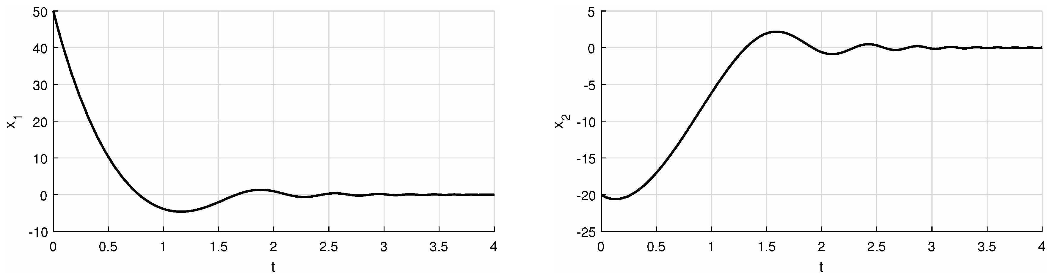
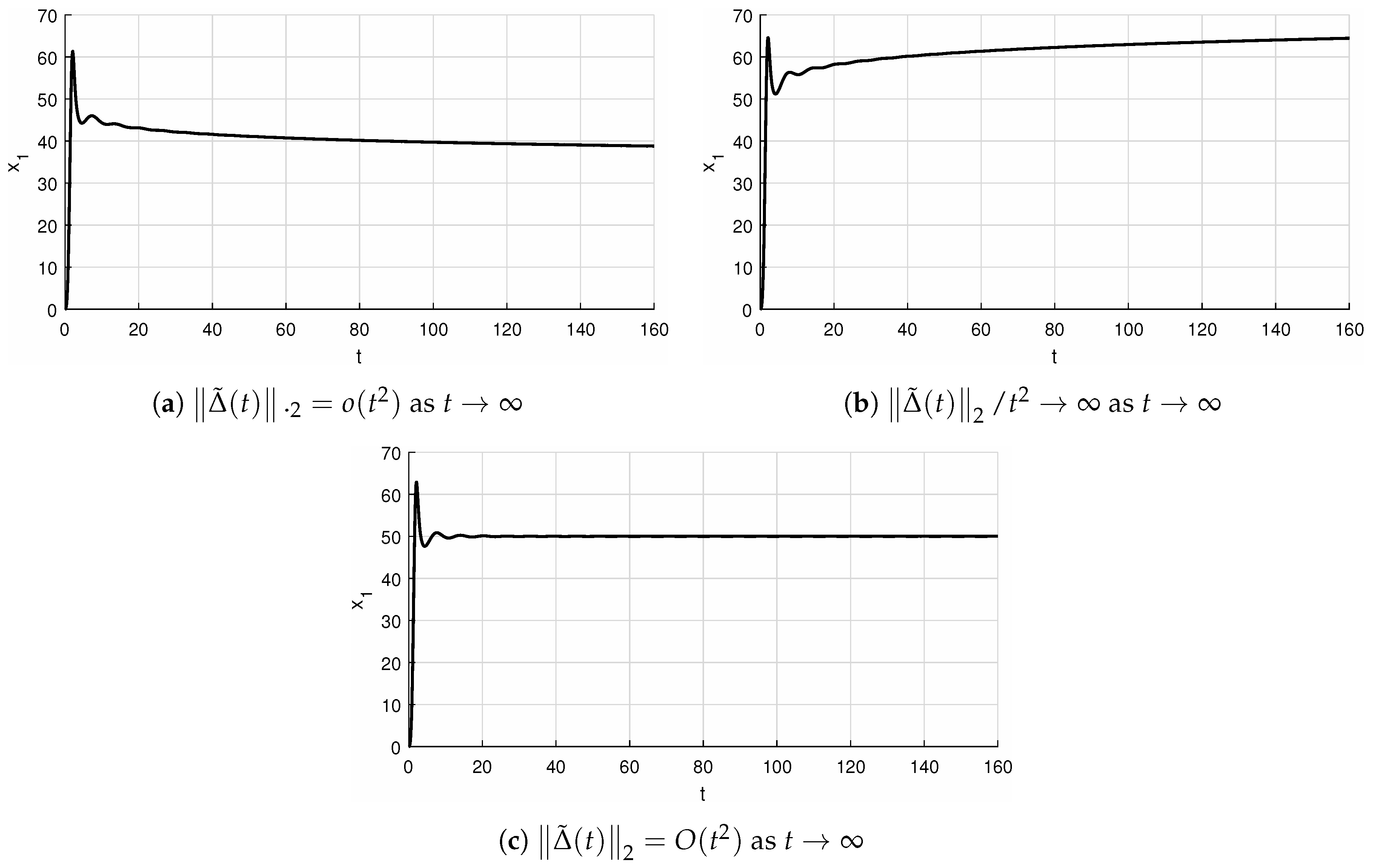
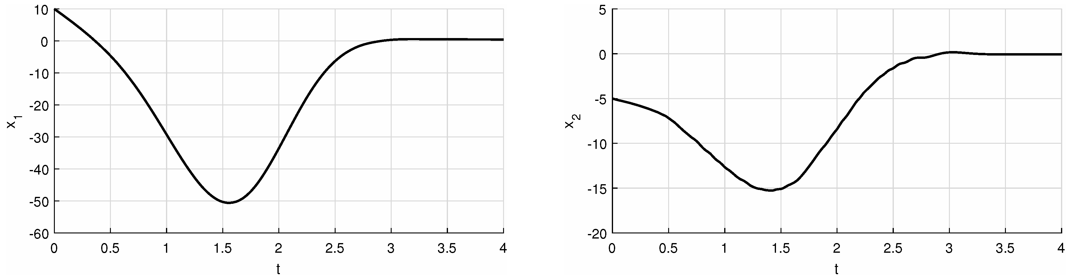
3. Simulation Experiments in MATLAB^®

Example 1.

To illustrate Theorem 1 with an example, let us consider the system

$$\dot{x}(t)=\underset{f(x(t),t)\equiv A(t)x(t)}{\underbrace{\left(\begin{array}{cc}-\lambda & \exp [t]\\ -\exp [t]& -\lambda \end{array}\right)x(t)}}+\delta (x,t),t\ge t_0,$$

(7)

with yet unspecified δ and parameter $\lambda \in \mathbb{R}.$ Obviously, in this specific example, ${\lambda }_{max}(t)={\lambda }_{min}(t)=-\lambda$ and Assumptions A1–A3 are satisfied if $\lambda >0$ and if ${∥\tilde{\mathsf{\Delta }}(t)∥}_2=o(1),$ that is, ${∥\tilde{\mathsf{\Delta }}(t)∥}_2\to 0$ as $t\to \infty .$

Simulation results for arbitrarily chosen $\lambda ,$ one representative $\delta (x,t)$ having these properties, and initial state $x(t_0)\in {\mathbb{R}}^n$ are shown in Figure 1 (the source code

Listing 1. MATLAB ^® code for Figure 1 (The MathWorks, Inc., 3 Apple Hill Drive, Natick, Massachusetts 01760 USA).

f = @(t,x) [(-2)*x(1)+(exp(t))*x(2)+(atan(x(1)+x(2))/(t+1));        (-exp(t))*x(1)+(-2)*x(2)+(exp(-t)/(x(1)^2+1))] [t,xa] = ode45(f,[0 4],[50 -20]); hold~on   pbaspect([2 1 1]) plot(t,xa(:,1), ’k’, ’LineWidth’,1.5) % 1 or 2 grid on xlabel(’t’) ylabel(’x_1’) % 1 or 2 print(’example_first_x_1’,’-deps’) % 1 or 2

).

Remark 3.

The condition ${∥\tilde{\mathsf{\Delta }}(t)∥}_2\to 0$ in Example 1 is only sufficient condition for convergence to zero of all solutions. Thus, the solutions can theoretically converge to zero also for the perturbations that do not satisfy that constraint. In fact, the fundamental matrix of $\dot{x}=A(t)x$ satisfies

$$X(t)=\exp [-\lambda t]\left(\begin{array}{cc}sin\left(\exp [t]\right)& \hfill -cos\left(\exp [t]\right)\\ cos\left(\exp [t]\right)& \hfill sin\left(\exp [t]\right)\end{array}\right),$$

$$X^{-1}(t)=\exp [\lambda t]\left(\begin{array}{cc}\hfill sin\left(\exp [t]\right)& cos\left(\exp [t]\right)\\ \hfill -cos\left(\exp [t]\right)& sin\left(\exp [t]\right)\end{array}\right)$$

and the solutions for some specific perturbations δ depending only on t can be calculated explicitly by using (6). For example, if $\delta (x,t)={(c,0)}^T,$ $c\in \mathbb{R}$ is constant, the solution of (7) with $\lambda =2$ and the initial state $x(t_0)=0,$

$$x(t)=\left(\begin{array}{c}c\exp [-2t]\left[\exp [t_0]sin\left(\exp [t]-\exp [t_0]\right)-cos\left(\exp [t]-\exp [t_0]\right)+1\right]\\ c\exp [-2t]\left[sin\left(\exp [t]-\exp [t_0]\right)-\exp [t]+\exp [t_0]cos\left(\exp [t]-\exp [t_0]\right)\right]\end{array}\right)\to 0$$

as $t\to \infty .$ On the other side, for another bounded perturbation

$$\delta (x,t)=\left(\begin{array}{c}sin\left(\exp [t]\right)\\ cos\left(\exp [t]\right)\end{array}\right)$$

the explicit solution for $\lambda =1,$

$$x(t)=\left[1-\exp [t_0-t]\right]\left(\begin{array}{c}sin\left(\exp [t]\right)\\ cos\left(\exp [t]\right)\end{array}\right)\to 0\mathrm{as}t\to \infty$$

because

$${∥x(t)∥}_2=\left[1-\exp [t_0-t]\right]\to 1\mathrm{as}t\to \infty .$$

This example showed that the coupled conditions on the system and perturbation in Theorem 1 cannot be weakened too much. Note, that the sine and cosine functions contained in the fundamental matrix are responsible for the "wavy" shape of the solutions of (7).

The following example illustrates the possibility that the system with time-varying linear part of nominal system can be robust also in the case of unbounded external disturbances affecting the system.

Example 2.

Let us consider the linear time-varying system

$$\dot{x}(t)=\left(\begin{array}{cc}-t^2+sin\left(t\right)& b\\ 0& 1-t^2+sin\left(t\right)\end{array}\right)x(t)+\delta (x,t),t\ge t_0,$$

(8)

where b is a real parameter. Stability analysis for time-varying linear systems and their robustness is of growing interest in the control community. One of the reasons for both researchers and practitioners is the growing importance of adaptive controllers for which underlying feedback closed-loop adaptive control system is time-varying and linear [35,36].

The eigenvalues of $\frac{1}{2}[A(t)+A^T(t)]$ are

$${\lambda }_1(t)=sin\left(t\right)+\frac{\sqrt{b^2+1}}{2}-t^2+\frac{1}{2},{\lambda }_2(t)=sin\left(t\right)-\frac{\sqrt{b^2+1}}{2}-t^2+\frac{1}{2}$$

and so Asumption A1 of Theorem 1 is satisfied for any fixed value of $b$.

By Theorem 1, all solutions of (8) tends to zero as $t\to \infty$ if perturbing term tends to infinity slower than $t^2,$ more precisely, if the upper bound of ${∥\delta (x,t)∥}_2,$ ${∥\tilde{\mathsf{\Delta }}(t)∥}_2=o(t^2);$ see Figure 2 for results of simulation experiment in the MATLAB^® environment (the source code

Listing 2. MATLAB^® code for Figure 2.

syms b b=5; f = @(t,x) [(-t^2+sin(t))*x(1)+(b)*x(2)+t^(1.5);        (0)*x(1)+(1-t^2+sin(t))*x(2)+3*cos(t*x(1)-x(2))] [t,xa] = ode45(f,[0 4],[10 -5]); hold~on   pbaspect([2 1 1]) plot(t,xa(:,1), ’k’, ’LineWidth’,1.5) % 1 or 2 grid on xlabel(’t’) ylabel(’x_1’) % 1 or 2 print(’example_second_x_1’,’-deps’) % 1 or 2

).

In Figure 3, we can notice the changes in the slope of the first component $x_1(t)$ of solutions for (8) with $\delta (x,t)={\left(50t^{1.95},{\delta }_2(x,t)\right)}^T$ (the top left sub-figure), $\delta (x,t)={\left(50t^{2.05},{\delta }_2(x,t)\right)}^T$ (the top right sub-figure) and the borderline case $\delta (x,t)={\left(50t^{2.00},{\delta }_2(x,t)\right)}^T,$ ${\delta }_2(x,t)=t{x}_1/(x_1^2+x_2^2+1)$ (the bottom sub-figure) in computer simulations of long time dynamics near the border ${∥\tilde{\mathsf{\Delta }}(t)∥}_2=o(t^2)$ as $t\to \infty .$

4. Conclusions

In this paper we have established in terms of eigenvalues of symmetric part of linear part of the nominal vector field $f(x,t)$ the sufficient conditions to maintain the origin $x=0\in {\mathbb{R}}^n$ “attractive” for a wide class of perturbed nonlinear systems $\dot{x}=f(x,t)+\delta (x,t),$ where the term $\delta$ aggregates all external disturbances affecting the system. As a result, we proved a new criterion for assessment of global robustness of nonlinear systems in the sense that all solutions of the perturbed system converge to zero as $t\to \infty$ as long as the perturbing term $\delta$ satisfies certain constraints given in Theorem 1.

References

1. Buscarino, A.; Fortuna, L.; Frasca, M. Experimental robust synchronization of hyperchaotic circuits. Phys. D Nonlinear Phenom. 2009, 238, 1917–1922. [Google Scholar] [CrossRef]
2. Fortuna, L.; Frasca, M. Optimal and Robust Control: Advanced Topics with MATLAB®; CRC Press: Boca Raton, FL, USA, 2012. [Google Scholar]
3. Buscarino, A.; Gambuzza, L.V.; Porfiri, M.; Fortuna, L.; Frasca, M. Robustness to Noise in Synchronization of Complex Networks; Scientific Reports 3; Nature Publishing Group: New York, NY, USA, 2013. [Google Scholar]
4. Buscarino, A.; Fortuna, L.; Frasca, M.; Iachello, M.; Pham, V.T. Robustness to noise in synchronization of network motifs: Experimental results. Chaos Interdiscip. J. Nonlinear Sci. 2012, 22, 043106. [Google Scholar] [CrossRef]
5. Gambuzza, L.V.; Buscarino, A.; Fortuna, L.; Porfiri, M.; Frasca, M. Analysis of dynamical robustness to noise in power grids. IEEE J. Emerg. Sel. Top. Circuits Syst. 2017, 7, 413–421. [Google Scholar] [CrossRef]
6. Ge, H.; Chen, G.; Yu, H.; Chen, H.; An, F. Theoretical Analysis of Empirical Mode Decomposition. Symmetry 2018, 10, 623. [Google Scholar] [CrossRef]
7. Yang, S.; Li, P.; Wen, H.; Xie, Y.; He, Z. K-Hyperline Clustering-Based Color Image Segmentation Robust to Illumination Changes. Symmetry 2018, 10, 610. [Google Scholar] [CrossRef]
8. Du, B.; Zhou, H. A Robust Optimization Approach to the Multiple Allocation p-Center Facility Location Problem. Symmetry 2018, 10, 588. [Google Scholar] [CrossRef]
9. Cao, Q.; Cao, C.; Wang, F.; Liu, D.; Sun, H. Robust Adaptive Full-Order TSM Control Based on Neural Network. Symmetry 2018, 10, 726. [Google Scholar] [CrossRef]
10. Yang, X.-B.; He, Y.-G.; Li, C.-L. Dynamics Feature and Synchronization of a Robust Fractional-Order Chaotic System. Complexity 2018, 2018, 8797314. [Google Scholar] [CrossRef]
11. Xu, X.; Xue, H.; Peng, Y.; Xu, Q.; Yang, J. Robust Exponential Stability of Switched Complex-Valued Neural Networks with Interval Parameter Uncertainties and Impulses. Complexity 2018, 2018, 4981812. [Google Scholar] [CrossRef]
12. Pérez-Cruz, J.H. Stabilization and Synchronization of Uncertain Zhang System by Means of Robust Adaptive Control. Complexity 2018, 2018, 4989520. [Google Scholar] [CrossRef]
13. Fang, S. Robust Impulsive Stabilization of Uncertain Nonlinear Singular Systems with Application to Transportation Systems. Math. Probl. Eng. 2018, 2018, 1893262. [Google Scholar] [CrossRef]
14. Rodríguez-Mata, A.E.; Flores, G.; Martínez-Vásquez, A.H.; Mora-Felix, Z.D.; Castro-Linares, R.; Amabilis-Sosa, L.E. Discontinuous High-Gain Observer in a Robust Control UAV Quadrotor: Real-Time Application for Watershed Monitoring. Math. Probl. Eng. 2018, 2018, 4940360. [Google Scholar] [CrossRef]
15. Zhang, J.-X.; Yang, G.-H. Adaptive asymptotic stabilization of a class of unknown nonlinear systems with specified convergence rate. Int. J. Robust Nonlinear Control 2019, 29, 238–251. [Google Scholar] [CrossRef]
16. Vrabel, R. Stabilisation and state trajectory tracking problem for nonlinear control systems in the presence of disturbances. Int. J. Control 2017. [Google Scholar] [CrossRef]
17. Petersen, I.R.; Tempo, R. Robust control of uncertain systems: Classical results and recent developments. Automatica 2014, 50, 1315–1335. [Google Scholar] [CrossRef]
18. Liu, K.-Z.; Yao, Y. Robust Control: Theory and Applications; John Wiley & Sons: Singapore, 2016. [Google Scholar]
19. Coddington, E.A.; Levinson, N. Theory of Ordinary Differential Equations; McGraw-Hill: New York, NY, USA, 1955. [Google Scholar]
20. Hartman, P. Ordinary Differential Equations, 2nd ed.; Classics in Applied Mathematics Series 38; Society for Industrial and Applied Mathematics: Philadelphia, PA, USA, 2002. [Google Scholar]
21. Chicone, C. Ordinary Differential Equations with Applications; Springer-Verlag New York, Inc.: New York, NY, USA, 1999. [Google Scholar]
22. Vrabel, R. On local asymptotic stabilization of the nonlinear systems with time-varying perturbations by state-feedback control. Int. J. Gen. Syst. 2019, 1, 80–89. [Google Scholar] [CrossRef]
23. Vrabel, R. Local null controllability of the control-affine nonlinear systems with time-varying disturbances. Eur. J. Control 2018, 40, 80–86. [Google Scholar] [CrossRef]
24. Pavlov, A.; Pogromsky, A.; van de Wouw, N.; Nijmeijer, H. Convergent dynamics, a tribute to Boris Pavlovich Demidovich. Syst. Control Lett. 2002, 52, 257–261. [Google Scholar] [CrossRef]
25. Khalil, H.K. Nonlinear Systems, 3rd ed.; Prentice-Hall: Englewood Cliffs, NJ, USA, 2002. [Google Scholar]
26. Sontag, E.D. Smooth stabilization implies coprime factorization. IEEE Trans. Automat. Control 1989, 34, 435–443. [Google Scholar] [CrossRef]
27. Sontag, E.D.; Wang, Y. On characterizations of the input-to-state stability property. Syst. Control Lett. 1995, 24, 1283–1294. [Google Scholar] [CrossRef]
28. Perko, L. Differential Equations and Dynamical Systems, 3rd ed.; Texts in Applied Mathematics 7; Springer-Verlag New York, Inc.: New York, NY, USA, 2001. [Google Scholar]
29. Slotine, J.-J.E.; Li, W. Applied Nonlinear Control; Prentice Hall: Englewood Cliffs, NJ, USA, 1991. [Google Scholar]
30. Vidyasagar, M. Nonlinear System Analysis, 2nd ed.; Prentice Hall: Englewood Cliffs, NJ, USA, 1993. [Google Scholar]
31. Rugh, W.J. Linear System Theory, 2nd ed.; Prentice-Hall: Upper Saddle River, NJ, USA, 1996. [Google Scholar]
32. Horn, R.A.; Johnson, C.R. Matrix Analysis; Cambridge University Press: Cambridge, UK, 1990. [Google Scholar]
33. Coppel, W.A. Stability and Asymptotic Behavior of Differential Equations; D. C. Heath and Company: Boston, MA, USA, 1965. [Google Scholar]
34. Harville, D.A. Matrix Algebra From a Statistician’s Perspective; Springer: New York, NY, USA, 2008. [Google Scholar]
35. Ioannou, A.; Sun, J. Robust Adaptive Control; Prentice-Hall: Upper Saddle River, NJ, USA, 1996. [Google Scholar]
36. Shamma, J.S.; Athans, M. Guaranteed properties of gain scheduled control for linear parameter-varying plants. Automatica 1991, 27, 559–564. [Google Scholar] [CrossRef]
Figure 1. Solution x ( t ) = x 1 ( t ) , x 2 ( t ) T of (7) for λ = 2 , δ ( x , t ) = arctan ( x 1 + x 2 ) ( t + 1 ) , exp [ t ] ( x 1 2 + 1 ) T and initial state x ( 0 ) = ( 50 , 20 ) T . Obviously, Δ ˜ ( t ) 2 = π / 2 t + 1 2 + exp [ 2 t ] = o ( 1 ) as t .
Symmetry 11 00569 g001
Figure 2. Solution x ( t ) = x 1 ( t ) , x 2 ( t ) T of (8) for b = 5 , δ ( x , t ) = t 3 / 2 , 3 cos t x 1 x 2 T and initial state x ( 0 ) = ( 10 , 5 ) T . Obviously, Δ ˜ ( t ) 2 = t 3 + 9 = o ( t 2 ) as t .
Symmetry 11 00569 g002
Figure 3. The solution component x 1 ( t ) of (8) for b = 5 , initial state x ( 0 ) = 0 and with (a) δ ( x , t ) = 50 t 1.95 , δ 2 ( x , t ) T satisfying Assumption 3 of Theorem 1, (b) δ ( x , t ) = 50 t 2.05 , δ 2 ( x , t ) T that does not satisfy Assumption 3 of Theorem 1 and (c) the borderline case, δ ( x , t ) = 50 t 2.00 , δ 2 ( x , t ) T , δ 2 ( x , t ) = t x 1 / ( x 1 2 + x 2 2 + 1 ) .
Symmetry 11 00569 g003