Neural Networks Application for Processing of the Data from the FMICW Radars

Abstract

In this paper the results of the Neural Networks and machine learning applications for radar signal processing are presented. The radar output from the primary radar signal processing is represented as a 2D image composed from echoes of the targets and noise background. The Frequency Modulated Interrupted Continuous Wave (FMICW) radar PCDR35 (Portable Cloud Doppler Radar at the frequency 35.4 GHz) was used. Presently, the processing is realized via a National Instruments industrial computer. The neural network of the proposed system is using four or five (optional for the user) signal processing steps. These steps are 2D spectrum filtration, thresholding, unification of the target, target area transforming to the rectangular shape (optional step), and target board line detection. The proposed neural network was tested with sets of four cases (100 tests for every case). This neural network provides image processing of the 2D spectrum. The results obtained from this new system are much better than the results of our previous algorithm.

1. Introduction

The radar PCDR 35 was developed for the Institute of Atmospheric Physics Czech Academy of Sciences. This radar is based on the industrial computer from the National Instruments company. The memory of this system is very limited. The secondary processing describes the data and only important information is saved (number of the targets, distances, reflected powers, Doppler shifts). We are describing the algorithm for the automatic evaluation of the signal from this radar by using neural networks. After comparison with our previous algorithm [1], The benefit of this algorithm is its simple implementation on the Field Programmable Gate Array (FPGA) system and thanks to this, we can analyze signals much faster.

2. FMICW Radar Description

The FMICW system works as a combination of the pulse radar and FMCW (Frequency Modulated Continuous Wave) radar. Examples of FMCW systems are described in [2,3]. The principle of the FMICW radar is described in [4], but this system was developed for the measurement of the ionosphere, and the pulse part of the system does not have a big influence on the signals. The block diagram of the FMICW radar is shown in Figure 1. The signal is generated by the sweeping generator and connected to the output amplifier. The switching of the system is realized via PIN diodes; one is for the connection to the transmitting amplifier and the second is for the receiver. A detailed description of the radar PCDR 35 blocks was realized in [5]. The radar PCDR 35 was developed for the measurement in short distances (less than 10 km) and we must include the influence of pulses in this case, as shown in Figure 2. Because we have different lengths of the reflected signals, we must do corrections of the power. An example of this was described in [5]. The distance in FMICW radars is calculated by Equation (1).

$$R=\frac{c_0·\delta f·T}{2·\Delta f}+e\left(\delta f\right),$$

(1)

where c₀ is the light speed, δf is the output frequency, T is the measurement period, ∆f is the sweep range and e(δf) is the measurement error.

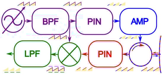
Figure 1. Block diagram of Frequency Modulated Interrupted Continuous Wave (FMICW) radar. [1].

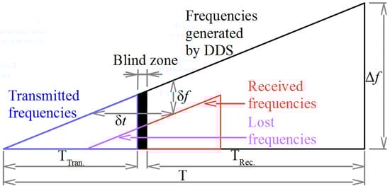
Figure 2. Timing diagram of FMICW radar. [6].

Frequencies are obtained during the primary signal processing of the radar. The frequency analysis can be realized by the non-parametric, or parametric methods [7]. The parametric AR model is described in [8]. More parametric and non-parametric methods are described in [9]. 2D FFT can be used for the estimation of the target velocities, this algorithm is described in [10,11]. The principle is shown in Figure 3. Measured data are sorted in a matrix after every measurement is transformed by the Fast Fourier Transform (FFT). The results from this process are the range profiles for the times of measurement. The next step is applying the FFT on the time dimension. This transformation changes the time dimensions to Doppler shift dimensions. The Doppler shift resolution is defined by Equation (2). The testing measurements of the radar PCDR 35 and sensitivity analysis were presented in [12]. Examples of four cases of 2D spectra are shown in Figure 4, where PSD is power spectral density. The clutter elimination is described in [13], where the static clutter detection and the meteorological clutter is canceled by the Airborne Moving Target Identification (AMTI) filter. It represents selected velocities for all distances in the case of the signal 2D spectrum.

$$\delta D=\frac{1}{T·N},$$

(2)

where T is the time between measurements (periods), and N represents the number of measurements.

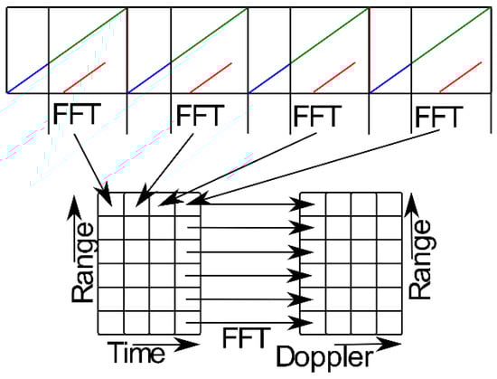
Figure 3. Principle of the 2D Fast Fourier Transform (FFT) from the signal. [10].

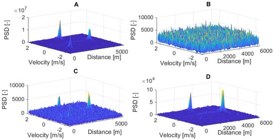
Figure 4. 2D spectra of the four situation cases: (A) 2D spectrum of the signals with three strong echoes, (B) 2D spectrum of the signals with noise only, (C) 2D spectrum of the signal with three weak echoes (D) 2D spectrum of the signal contains one weak and two strong echoes.

3. Neural Networks

The neuron model is shown in Figure 5. We can see, that the neuron has N inputs $(x_1,...,x_N)$ () and one output $(y)$. Every input is multiplied by the input weight $(w_1,...,w_N)$, this value changes during the learning process. The output has application function $Y$, which decides the output value. Activation functions can be different and usually are nonlinear (signum function, limited linear function, standard logistic function, hyperbolic tangents). Examples of these functions are described in [14]. The neuron bias is represented by the input $b$, and this signal is also multiplied by weight $w_0$. If we look at the neuron model, we can see that the neuron is based on principles of digital filters. The mathematical description of one neuron is in Equation (3). The benefit of this model is the easy application on the FPGA with faster processing speed. Applications of the neurons and neural networks on the FPGA are described in [15].

$$y_j=Y_j\left(b·w_{0j}+{\displaystyle \sum _{i=1}^N\left\{w_{ij}·x_{ij}\right\}}\right),$$

(3)

where $Y_j$ is the application function of a neuron, $x_{ij}$ represents i-th neuron input, $w_{ij}$ represents the weight for the input (synapse), b represents bias and $N$ represents number of inputs.

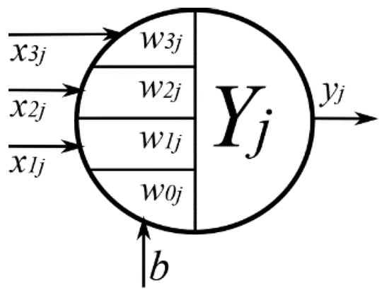
Figure 5. Formal neuron with bias [16].

The Hebbian learning is based on the increasing and decreasing connections between two neurons (changing of the input weights). The increasing and decreasing is, in turn, controlled by the inputs and outputs. Training signals are used in the learning sequence. Results are set by the user and if input and output are related, then the connection strengthens (the weight is increased), but if they are not related, the connection weakens (the weight is decreased). This style is called learning with a teacher. If we use all combinations, the system remembers all solutions.

The neural network is composed of the basic neurons. Neurons can be sorted into more layers. These layers are sorted into groups known as the input layer, hidden layers and output layer. An example of the neuron network in topology (3-3-4-2) is shown in Figure 6. This is the neural network with more layers. The connection between neurons can skip to any layer or can be realized as the back loop.

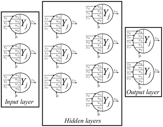
Figure 6. An example of a multilayer neural network architecture (3-3-4-2).

4. Application of the Neural Networks for the Radar Signal Processing

The neural network for our algorithm is composed of three, or four layers (optional). Every layer has a specific function. The input layer is for the 2D spectrum filtration and the thresholding. The second layer is for the target unification when any target is split. The third layer can be a transformation of the target area to the rectangular shape (this layer is optional). The last layer is the target board line detection.

4.1. Filtration and Thresholding

Neurons in this layer transform the 2D spectrum (the original spectrum is represented by the size of the spectral components) to a binary matrix, where 1 represents the positive detection and −1 represents the negative detection in the tested cell. In this layer there are used two types of neurons, one type is used for the filtration and the second type is used for the threshold value estimation. This value is used in the filtration neurons for the activation function. From this, it is obvious that the numbers of neurons for the filtration and the thresholding in the input layer are functions of the 2D spectrum size. The model of this neuron is shown in Figure 7. Input signals are in the input vector ${\overrightarrow{X}}_j$. This vector has $n$ elements and these elements are obtained from the distance profile. Synapses are saved in the vector ${\overrightarrow{W}}_j$, and activation function $Y_j$ is the signum function. The neuron’s model for the threshold value estimation is shown in Figure 8. The activation function $Y_j$ of this neuron is linear, the input is the matrix of the 2D spectrum from the radar measured data. This neuron has common weight for all inputs because all inputs have the same priority. This neuron definition is shown in Equation (4), where $TV$ represents the threshold value (5).

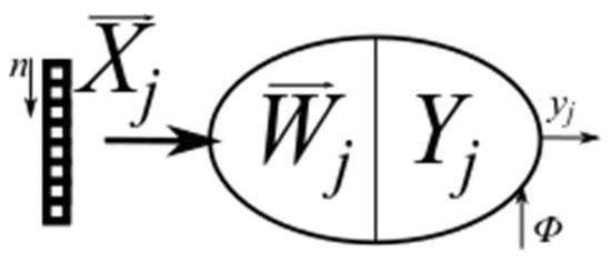
Figure 7. Neuron for the filtration and thresholding.

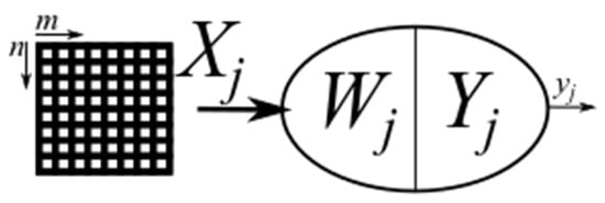
Figure 8. Neuron for the threshold level estimation.

Teaching the neurons is described in the algorithm in Figure 9. The 2D spectrum is manually processed and transformed into the mask, where 1 represents positive detection (target) and −1 represents negative detection (noise). This mask is used for the neural network Hebbian learning. As described in Figure 7, the input vector is obtained from the 2D spectrum. The used vector has 21 elements and all inputs have the same Doppler shifts. Weights are increased in the case of positive detection 1 and decreased in the case of negative detection −1. The first threshold value is estimated according to Equation (5). At the start of the algorithm, the weight is chosen as 1. The next step is 2D spectrum processing by using the neural network and the obtained result is compared with the mask. If the results match, the algorithm is finished. If the results do not match, the weight is modified according to the results. If the neural network does not detect any targets, the weight is divided by 1.4 and if the neural network generates false alerts, the signal is multiplied by 1.4 (this value was chosen experimentally). The next step is the threshold value recalculation from the new weight and the 2D spectrum is processed again.

$$y_j=Y_j\left(w_j·{\displaystyle \sum _{i=1}^N\left\{x_{ij}\right\};TV}\right),$$

(4)

$$TV=w_j·{\displaystyle \sum _{n=1}^N{\displaystyle \sum _{m=1}^M\left\{2DFF{T}_{nm}\right\}}},$$

(5)

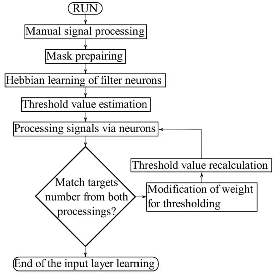
Figure 9. Algorithm for the learning of the input layer of the neural network for the radar signal processing.

After the input network learning, we will obtain weight parameters for the filtration neurons. These weights are shown in the graph in Figure 10, and these parameters will be set by Equation (3). Weights are saved in vector ${\overrightarrow{W}}_J$ from Figure 7. The weight for the neuron threshold value estimation was estimated from the learning as 113.3817189 × 10⁻⁶. A test of the layer application is shown in Figure 11. The 2D spectrum with three targets was used for input to this layer.

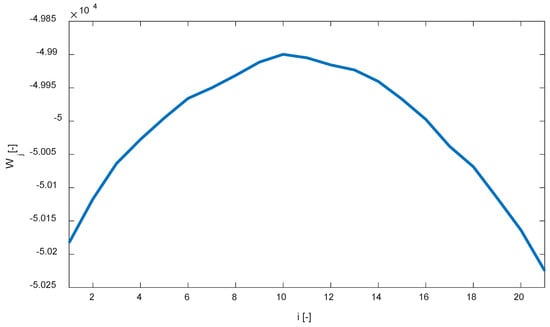
Figure 10. Synapses weight vector parameters for filtration of the 2D spectra. (20 inputs).

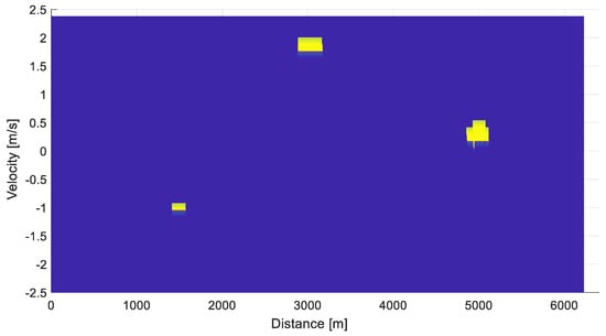
Figure 11. Test of the neurons in the input layer (filtration and thresholding of the 2D spectrum): 2D spectrum with two strong echoes and one weak echo is used for input in this figure.

4.2. Unification of the Targets

The target can be split during the thresholding process, and we must make target unification in this case. For this, we are using neural sub-networks. One of these neural networks is shown in Figure 12. Neurons in the first layer are described by Equation (6) and the output layer is described by Equation (7). For all neurons, the activation function signum is used. Input signals are two vectors of five elements. The first vector has elements placed before the tested element in the range dimension, and the second input vector has elements following the tested element in the range dimension. The neuron in the second layer is the OR function with three inputs, where one input is the cell state before the unification process and the next two inputs are outputs from the first layer neurons. During the Hebbian learning, we used a negative combination twice for the better setting. A test of this neural sub layer is shown in Figure 13, where we can see that both splits were removed, and the target is again united.

$$y_j=Y_j\left({\displaystyle \sum _{i=1}^5\left\{x_{ij}\right\}+4}\right),$$

(6)

$$y_j=Y_j\left(3·{\displaystyle \sum _{i=1}^2\left\{x_{ij}\right\}+5}\right),$$

(7)

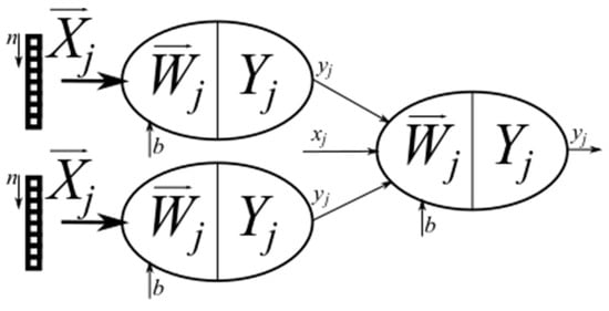
Figure 12. Neural network for unification of the targets.

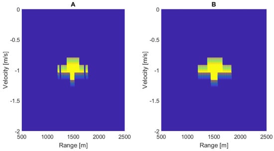
Figure 13. Test of the neural sub network for unification of the targets: (A) Target is split to three parts (B) Target was restore via neural sub network.

4.3. Detection of the Target Board Lines

The neurons, with nine inputs in this layer, are organized in the 3 × 3 matrix of elements. Inputs are connected from layer 1 (inputs can be 1, or −1). The activation function is the signum function. The model of this neuron is similar to the neuron from Figure 8, only another activation function and different bias are used. This layer is used for the definition of the target board lines. The neuron tests if the middle element is −1 and if there are any elements with 1 around. If these conditions are not successful, the output is −1. If conditions are successful, the output is 1. After the Hebbian learning we obtained an equation, which cannot be used, because in the case when all inputs are −1 the output is wrong. The layer generated the positive board line of the target and the first condition was not successful. Then we used this case more times for the Hebbian learning and we trained this neural network until the neural network started to analyze this case correctly. We obtained Equation (8) from this training. Input x_9j represents the middle element in the matrix 3 × 3, the weight for this element is −8, the weight for the other elements is 1. This is because these elements have the same priority and the value −0 is for bias (for the Hebbian learning we were using eight cases for positive detection and eight cases for negative detection). Application of this layer is shown in Figure 14. Input for testing of this layer is the output from the thresholding layer, which was shown in Figure 11 after the unification of the targets. We can see that the 2D spectrum was analyzed correctly.

$$y_j=Y_j\left(-8·w_{9j}+{\displaystyle \sum _{i=1}^8\left\{x_{ij}\right\}-0}\right),$$

(8)

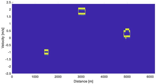
Figure 14. Board lines of the targets detected in the output from the unification neural sub network.

4.4. Marking of the Targets Position

This part is used for the target marking in the signal. The processing is composed of the two steps. The first step is the transformation of the target area and the settings of the rectangular shape. The second step is the board lines detection in the rectangular shape.

The neural sub-network for the transformation of the area is shown in Figure 15. The first layer is from neurons described by Equation (9). This is the OR function which depends on the vector length. For the Doppler shift dimension, a vector where n is 21 elements is used, and for the range dimension, a vector where m is 81 elements is used. The tested element is in the vector middle in both cases. The equation for the OR neurons which are used for the transformation of the area is described by (9). It was derived from the Hebbian learning for more lengths of the input vectors. The output layer is the AND neuron, which is described by Equation (10). The signum function is used for both neuron types in this neural sub-network. For the second step, the same layer is used as in the case when we detected the board lines of the targets after the thresholding. The output from the application of this layer is shown in Figure 16.

$$y_j=Y_j\left({\displaystyle \sum _{i=1}^I\left\{x_{ij}\right\}+I-1}\right),$$

(9)

$$y_j=Y_j\left({\displaystyle \sum _{i=1}^2\left\{x_{ij}\right\}-1}\right),$$

(10)

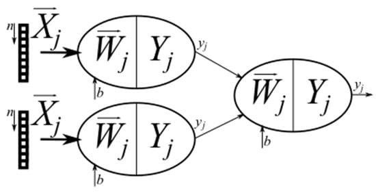
Figure 15. Neural sub network for transforming of the area to rectangular shape.

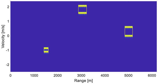
Figure 16. Board lines of the targets (rectangular shape) in the output from the proposed system. One weak and two strong echoes were in the input.

5. Description of the Proposed Neural Network

Proposed parts of the neural network were connected to the final system. This final neural network is shown in Figure 17. Neurons placed in the rectangular shape represent this neuron matrix, and outputs from the neural network are realized by the marking blocks. The input matrix size is 665 × 41 elements (665 elements represent the samples of one measurement, it is the function of the sampling frequency and radar range. Forty-one samples represent the realizations, fewer samples are not enough for Doppler measurements, more samples make long response time of the system). The output signal is the matrix with the same dimensions. The processed signals example is shown in Figure 18. The targets in the 2D spectrum were marked by the red lines. The case in the right top position is only with noise and no target is marked.

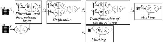
Figure 17. Neural network proposed for the FMICW radar signal processing.

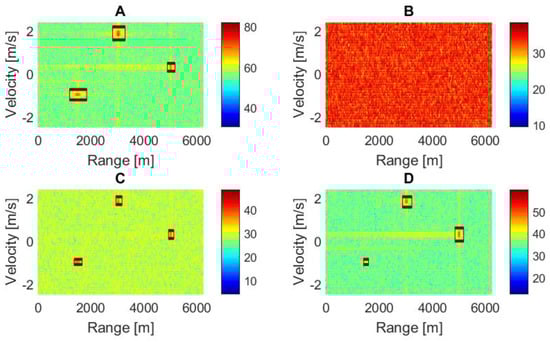
Figure 18. Marking of the targets in 2D spectrum: (A) processing of the signal with three strong echoes, (B) processing of the signal without echoes, (C) processing of the signal with three weak echoes and (D) processing of the signal with one weak and two strong echoes.

6. The Algorithm Test on the Training Sequence Data and Discussion

The proposed neural network was tested on the simulated data. These data were created by our simulator, which is based on the real system PCDR 35. Real measurement data and a comparison with simulated data is shown in [17]. In the results, there is a difference, where the measured data contains a noise level which is dependent on the distance, and this is not reflected in the simulator. This is caused by the wrong impedance in the radar output, but this was corrected in cooperation with the BTV Klimkovice company.

Results of the proposed neural network are presented in Table 1. We tested the neural network in four cases: three strong targets, noise, three weak targets, and one weak with two strong targets. For every tested case, 100 sets of the simulated data were used. From Table 1 we can see very good results. Table 2 is added for comparison, where the unification layer in the neural network was not used. We can see, that the results are unacceptable. For the test, the same data were used, which we used for the validation of our previous algorithm, which is published in [1]. The algorithm results are in Table 3. From the comparison of Table 1 and Table 3, we can see that the neural network results are much better than the previous algorithm in two cases, and the same results are in the next two cases.

Table 1. Results of the proposed neural network.

Cases	Totally Right	Lost Targets	False Alerts
3 strong targets	97	0	3
Noise	100	-	0
3 weak targets	96	4	4
1 weak and 2 strong targets	94	0	6

Table 2. Results of the proposed neural network without unification of the targets.

Cases	Totally Right	Lost Targets	False Alerts
3 strong targets	33	0	77
Noise	100	-	0
3 weak targets	95	4	5
1 weak and 2 strong targets	94	0	6

Table 3. Validation of the previous algorithm published in [1].

Cases	Number of Targets	Distances	Doppler Shifts
3 strong targets	94	94	94
Noise	100	-	-
3 weak targets	96	96	96
1 weak and 2 strong targets	84	84	84

After revision of the wrongly processed cases, we found that false alerts in the case of three strong targets were caused by the usage of short vectors for the target unification. We tried to extend these vectors, and we used Equation (11) for the input into this neural sub-network. After the test, we obtained results from Table 4. We can see that the results are better for this target type, but from the process, we can estimate that in any case where the distance between the main target and the side lobe of this target can be bigger, we will obtain the wrong results again. We also cannot use a much longer vector length, because we can do the unification of more targets to the one target. We can see that these results are good; processing can contain errors, but these mistakes are rare. After checking the wrongly processed cases for the last situation, we can see that the distance between the original target position and the detected side lobe is very big and cannot be removed by the neural sub network for unification. One example is shown in Figure 19. When we checked the lost targets, we observed that targets were lost, because the simulated target position was the only one point from the area. This marking causes the target loss because the area is very small in this case. If we include board lines to the target area, the target is marked correctly. Thanks to this we can obtain results in Table 5. Targets are detected correctly, only they are not in the middle of the marked area. From this, we can see that the used neural network has much better results than previous algorithms.

$$y_j=Y_j\left({\displaystyle \sum _{i=1}^7\left\{x_{ij}\right\}+6}\right),$$

(11)

Table 4. Modification of the neural network for improving the strong target detections.

Cases	Totally Right	Lost Targets	False Alerts
3 strong targets	100	0	0
Noise	100	-	0
3 weak targets	96	4	4
1 weak and 2 strong targets	94	0	6

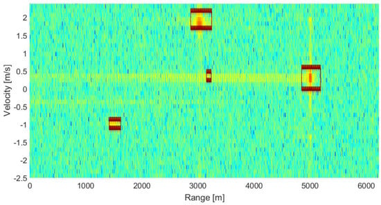
Figure 19. False alert in the processed 2D spectrum.

Table 5. Modification of the neural network for improving the weak targets detection.

Cases	Totally Right	Lost Targets	False Alerts
3 strong targets	100	0	0
Noise	100	-	0
3 weak targets	100	0	0
1 weak and 2 strong targets	94	0	6

An example of another work in this field can be found in [18]. These authors measure the position and Doppler shifts of the targets in this research. They are using the CFAR (constant false alarm rate) method for detection and tracking of the target. The setting of their algorithm and the evaluation study are not published. Another approach is used in [19], where other authors use another type of the algorithm for the processing of the velocity measurement. The second group of authors are using target route tracking for velocity estimation of the targets in this research, but they did not describe their algorithm exactly. From the results which they published, we can see that they also have problems with false alerts and losing the targets. The efficiency of this algorithm was not published. Better research on this topic is described in [20]. Here, the authors described their algorithm and made an evaluation of the success. Their algorithm has, according to tests, very good results. These results are comparable with our algorithm except for Doppler shifts or velocities. This is because they did not include these measurements in their research.

7. Conclusions

In this paper, we described the neural network for the FMICW radar signal processing. The neural network can be easily used for implementation on the FPGA with the speed processing benefit. Use of the neural network improved the threshold level estimation. Before, we used the median, and it was very time-consuming in comparison with the neural network, where the sum of elements is multiplied by the weight. This way is faster for PC processing in comparison with the previous way.

The two outputs are from the neural network; one for the precision marking of the targets and one for the marking by the rectangular shape. The first output is better for extremely big target detection (the rain cell). The second one is good for the point targets. Because we tested this neural network with the same data as our older algorithm, we can easily compare these two approaches for radar signal processing. From the results, we can see that the usage of this neural network is much better than our previous algorithm. In the case of one weak and two strong targets, the improvement is around 10%.

References

- Rejfek, L.; Fiser, O.; Chmelar, P.; Pitas, K.; Bezousek, P.; Phuong, T.T.; Dong, S.T.C.H. Automatic Analysis of the Signals from the FMICW Radars. In Proceedings of the 2019 29th International Conference Radioelektronika (RADIOELEKTRONIKA), Pardubice, Czech Republic, 16–18 April 2019; pp. 1–4. [Google Scholar] [CrossRef]
- Neemat, S.; Krasnov, O.; Yarovoy, A. An interference mitigation technique for FMCW radar using beat-frequencies interpolation in the STFT domain. IEEE Trans. Microw. Theory Tech. 2019, 67, 1207–1220. [Google Scholar] [CrossRef]
- Bezousek, P.; Hajek, M.; Pola, M. Effects of signal distortion in a FMCW radar on range resolution. In Proceedings of the 15th Conference on Microwave Techniques (COMITE 2010), Brno, Czech Republic, 19–21 April 2010; pp. 113–116. [Google Scholar]
- Nozaki, K. FMCW Ionosonde for the SEALION project. J. Natl. Inst. Inf. Commun. Technol. 2009, 56, 287–298. [Google Scholar]
- Rejfek, L.; Fiser, O.; Matousek, D.; Beran, L.; Chmelar, P. Correction of received power for Doppler measurements by FMICW radars. In Proceedings of the Elmar—International Symposium Electronics in Marine 2017, Zadar, Croatia, 18–20 September 2017; pp. 107–110. [Google Scholar]
- Rejfek, L.; Bezousek, P.; Fiser, O.; Brazda, V. FMICW radar simulator at the frequency 35.4 GHz. In Proceedings of the 2014 24th International Conference Radioelektronika, RADIOELEKTRONIKA, Bratislava, Slovakia, 15–16 April 2014. [Google Scholar]
- Smekal, Z. Číslicové Zpracování Signálů; Skriptum; Vysoké Učení Technické v Brně, Fakulta Elektrotechniky a Komunikačních Technologií: Brno, Czech Republic, 2009; p. 208. [Google Scholar]
- Chmelarova, N.; Tykhonov, V.A. Composite vector stochastic processes model in the task of signals’ recognition. In Proceedings of the 2016 26th International Conference Radioelektronika, RADIOELEKTRONIKA, Kosice, Slovakia, 19–20 April 2016; pp. 203–206. [Google Scholar]
- Stoica, P.; Mosses, R. Introduction to Spectral Analysis; Prentice Hall: Upper Saddle River, NJ, USA, 1997. [Google Scholar]
- Otto, T. Presentation “Principle of FMCW Radars”. Available online: https://www.slideshare.net/tobiasotto/principle-of-fmcw-radars (accessed on 26 July 2012).
- Sediono, W. Method of measuring Doppler shift of moving targets using FMCW maritime radar. In Proceedings of the 2013 IEEE International Conference on Teaching, Assessment and Learning for Engineering (TALE), Bali, Indonesia, 26–29 August 2013; pp. 378–381. [Google Scholar]
- Rejfek, L.; Fiser, O.; Matousek, D.; Beran, L.; Chmelar, P. Sensitivity analysis of PCDR35 radar. In Proceedings of the Elmar—International Symposium Electronics in Marine, Zadar, Croatia, 18–20 September 2017; pp. 111–114. [Google Scholar]
- Reznicek, M.; Bezousek, P.; Zalabsky, T. AMTI filter design for radar with variable pulse repetition period. J. Electr. Eng. 2016, 67, 131–136. [Google Scholar]
- Hikawa, H. A Digital Hardware Pulse-Mode Neuron With Piecewise Linear activation Function. IEEE Trans. Neural Netw. 2003, 14, 1028–1037. [Google Scholar] [CrossRef] [PubMed]
- Liu, Y.; Liu, S.; Wang, Y.; Lombardi, F.; Han, J. A Stochastic Computational Multi-Layer Perceptron with Backward Propagation. IEEE Trans. Comput. 2018, 67, 1273–1286. [Google Scholar] [CrossRef]
- Volna, E. Scriptum “Neuronové sítě 1”; Ostravská Univerzita: Ostrava, Czech Republic, 2002. [Google Scholar]
- Mandlik, M.; Brazda, V. FMICW radar simulator. In Proceedings of the 25th International Conference Radioelektronika (RADIOELEKTRONIKA), Pardubice, Czech Republic, 21–22 April 2015; pp. 317–320. [Google Scholar]
- Krejci, T.; Mandlik, M. Close vehicle warning for bicyclists based on FMCW radar. In Proceedings of the 2017 27th International Conference Radioelektronika (RADIOELEKTRONIKA), Brno, Czech Republic, 19–20 April 2017; pp. 1–5. [Google Scholar]
- Hong, D.; Yang, C. Algorithm design for detection and tracking of multiple targets using FMCW radar. In Proceedings of the Program Book—OCEANS 2012 MTS/IEEE Yeosu: The Living Ocean and Coast—Diversity of Resources and Sustainable Activities, Yeosu, Korea, 21–24 May 2012. [Google Scholar]
- Yulian, D.; Hidayat, R.; Nugroho, H.A.; Lestari, A.A.; Prasaja, F. Automated ship detection with image enhancement and feature extraction in FMCW marine radars. In Proceedings of the 2017 International Conference on Radar, Antenna, Microwave, Electronics, and Telecommunications (ICRAMET), Jakarta, Indonesia, 23–24 October 2017; pp. 58–63. [Google Scholar]
© 2019 by the authors. Licensee MDPI, Basel, Switzerland. This article is an open access article distributed under the terms and conditions of the Creative Commons Attribution (CC BY) license (http://creativecommons.org/licenses/by/4.0/).