On Topological Properties of Symmetric Chemical Structures

Abstract

The utilizations of graph theory in chemistry and in the study of molecule structures are more than someone’s expectations, and, lately, it has increased exponentially. In molecular graphs, atoms are denoted by vertices and bonds by edges. In this paper, we focus on the molecular graph of (2D) silicon-carbon $S{i}_2{C}_3$-I and $S{i}_2{C}_3$-$II$. Moreover, we have computed topological indices, namely general Randić Zagreb types indices, geometric arithmetic index, atom–bond connectivity index, fourth atom–bond connectivity and fifth geometric arithmetic index of $S{i}_2{C}_3$-I and $S{i}_2{C}_3$-$II$.

1. Introduction

Every structural formula that includes covalent bonded compounds or molecules are graphs. Along these lines, they are called molecular graphs. Recently, chemical graph theory tools are used for numeration, systematization of the problem in hand, it provides the process of arranging laws or rules according to a system or planning, nomenclature, it provides the connection between the compounds or atoms, and computer programming. The significance of graph theory tools for science stands for the most part from the presence of isomerism, which is excused by substance diagram hypothesis. The pith of chemistry is the combinatorics of molecules as per clear principles. Along these lines, the most satisfactory numerical apparatuses for this design are graph hypothesis and combinatorics, the branches of arithmetic that are nearly related.

Silicon has numerous preferences over other semiconductor materials: It is, of minimal effort, it is nontoxic, essentially its accessibility is boundless, and behind it many years of involvement in purging, development and gadget creation. It is utilized for all cutting edge electronic gadgets.

The most reliable structures of two-dimensional (2D) silicon-carbon monolayer mixes with different stoichiometric blends were expected in [1] which in light of the molecule swarm streamlining signified as (PSO) method joined with thickness utilitarian hypothesis optimization.

The graphene sheets were effectively confined in [2,3] and from that point forward this honeycomb organized 2D material has roused and enlivened concentrated research interests to a great extent as a result of its surprising mechanical, electronic and optical properties, including its anomalous quantum Lobby influence, overwhelming electronic conductivity, and high mechanical quality. In particular, the intriguing electronic properties of graphene pull in see for this 2D material as a potential probability for applications in speedier and smaller electronic gadgets.

Like carbon, silicon additionally has a 2D allotrope with a honeycomb structure, in particular silicene. To date, bunches of exertion have been given to open a bandgap in silicene sheets. In addition, 2D silicon–carbon $(Si-C)$ monolayers can be seen as creation tunable materials between the unadulterated 2D carbon monolayer-graphene and the unadulterated 2D silicon monolayer-silicene. Loads of endeavors have been directed towards anticipating the most stable structures of the $SiC$ sheet read this [4,5] for more data.

Given a graph $G=(V,E)$ where V is the vertex set and E is the edge set of G, the degree $deg\left(s\right)$ of s is the quantity of spokes in G episode with s and is indicated as $d\left(s\right)$. A graph can be spoken to by a polynomial, a numerical esteem or by lattice frame. All the concepts of graph theory and combinatorics are used from the book of Harris et al. [6]. There are sure kinds of topological records for the most part capricious based, degree based and remove based files and so forth.

In 1975, $Milan$ Randić [7] introduced the randic index as below:

$$R_{-\frac{1}{2}}\left(G\right)=\sum _{st\in E\left(G\right)}\frac{1}{\sqrt{d\left(s\right)d\left(t\right)}}.$$

In 1988, Bollobás et al. [8] and Amic et al. [9] introduced the general Randić index independently. For more details about Randić index, its properties and important results, see [10,11,12,13]. The general Randić index is defined as:

$$R_{\alpha }\left(G\right)=\sum _{st\in E\left(G\right)}{\left(d\left(s\right)d\left(t\right)\right)}^{\alpha }.$$

Estrada et al. [14] defined atom–bond connectivity index as:

$$ABC\left(G\right)=\sum _{st\in E\left(G\right)}\sqrt{\frac{d\left(s\right)+d\left(t\right)-2}{d\left(s\right)d\left(t\right)}}.$$

The geometric arithmetic index $GA$ is introduced by Vukičević et al. [15] as:

$$GA\left(G\right)=\sum _{st\in E\left(G\right)}\frac{2\sqrt{d\left(s\right)d\left(t\right)}}{d\left(s\right)+d\left(t\right)}.$$

The Zagreb indices were introduced by Gutman and Trinajestic in [16,17]. For more details about Zagreb indices, its properties and important results, see [18,19,20]:

$$M_1\left(G\right)=\sum _{st\in E\left(G\right)}(d\left(s\right)+d\left(t\right)),$$

$$M_2\left(G\right)=\sum _{st\in E\left(G\right)}\left(d\left(s\right)d\left(t\right)\right).$$

Ghorbhani et al. [21] introduced the fourth version of atom–bond connectivity index $AB{C}_4$ as:

$$AB{C}_4\left(G\right)=\sum _{st\in E\left(G\right)}\sqrt{\frac{S\left(s\right)+S\left(t\right)-2}{S\left(s\right)S\left(t\right)}},$$

where $S\left(s\right)={\sum }_{st\in E\left(G\right)}d\left(t\right)$ and $S\left(t\right)={\sum }_{st\in E\left(G\right)}d\left(s\right)$. For more details about the fourth version of atom–bond connectivity index, its properties and important results, see [9,22,23,24,25].

Graovoc et al. [26] introduced the fifth version of geometric arithmetic index $G{A}_5$ as:

$$G{A}_5\left(G\right)=\sum _{st\in E\left(G\right)}\frac{2\sqrt{S\left(s\right)S\left(t\right)}}{S\left(s\right)+S\left(t\right)}.$$

2. Applications of Topological Indices

The Randic index is a topological descriptor that has correlated with a lot of chemical characteristics of the molecules and has been found to the parallel to computing the boiling point and Kovats constants of the molecules. The atom–bond connectivity $\left(ABC\right)$ index provides a very good correlation for the stability of linear alkanes as well as the branched alkanes and for computing the strain energy of cyclo alkanes [14]. To correlate with certain physico-chemical properties, $GA$ index has much better predictive power than the predictive power of the Randic connectivity index [27]. The first and second Zagreb index were found to occur for computation of the total $\pi$-electron energy of the molecules within specific approximate expressions [28]. These are among the graph invariants, who were proposed for measurement of skeleton of branching of the carbon-atom [17].

3. Methods

To compute our results, we use the method of combinatorial computing, vertex partition method, edge partition method, graph theoretical tools, analytic techniques, degree counting method and sum of degrees of neighbours method. Moreover, we use the Matlab for mathematical calculations and verifications. We also use the maple for plotting these mathematical results.

4. Silicon Carbide $S{i}_2{C}_3$-$I[p,q]$ 2D Structure

The 2D molecular graph of Silicon Carbide $S{i}_2{C}_3$-I is given in Figure 1. To describe its molecular graph, we have used the settings in this way: we define p as the number of connected unit cells in a row (chain) and by q we represents the number of connected rows each with p number of cell. In Figure 2, we gave a demonstration how the cells connect in a row (chain) and how one row connects to another row. We will denote this molecular graph by $S{i}_2{C}_3$-$I[p,q]$. Thus, the quantity of vertices in this graph is $10pq$ and the number of edges are $15pq-2p-3q$.

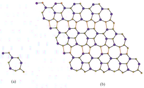
Figure 1. 2D structure of $S{i}_2{C}_3$-$I[p,q]$, (a) chemical unit cell of $S{i}_2{C}_3$-$I[p,q]$; (b) $S{i}_2{C}_3$-$I[4,3]$. Carbon atom C are brown and Silicon atom $Si$ are blue.

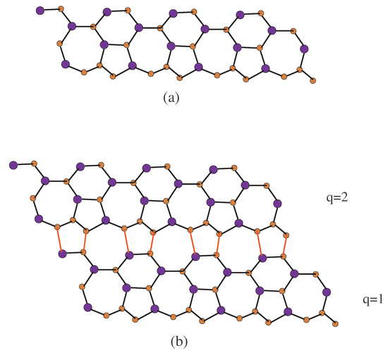
Figure 2. 2D structure of $S{i}_2{C}_3$-$I[p,q]$, (a) $S{i}_2{C}_3$-$I[4,1]$, one row with $p=4$ and $q=1$; (b) $S{i}_2{C}_3$-$I[4,2]$, two rows are being connecting. Red lines (edges) connects the upper and lower rows.

4.1. Methodology of Silicon Carbide $S{i}_2{C}_3$-$I[p,q]$ Formulas

For the computation of these formulas for Silicon Carbide $S{i}_2{C}_3$-$I[p,q]$, we use first a unit cell and then combine with another unit cell in horizontal direction and so on up to p unit cells. After this, we use first a unit cell and then combine with another unit cell in the vertical direction and so on up to q unit cells. Thus, we obtained Silicon Carbide $[p,q]$ structure (see Figure 1). Now, for the computation of vertices, we use the Table 1 and Matlab software for generalizing these formulas of vertices. In the following table, $V_1$ represents the quantity of vertices of degree 1, $V_2$ represents the quantity of vertices of degree 2 and $V_3$ represents the quantity of vertices of degree 3.

Table 1. Vertex partition of $S{i}_2{C}_3$-$I[p,q]$.

$[\mathit{p},\mathit{q}]$	$[1,1]$	$[1,2]$	$[1,3]$	$[2,1]$	$[2,2]$	$[2,3]$	$[3,1]$	$[3,2]$	$[3,3]$	$[4,1]$	$[4,2]$	$[4,3]$
$V_1$	2	2	2	2	2	2	2	2	2	2	2	2
$V_2$	6	12	18	10	16	2	14	20	26	18	28	30
$V_3$	2	6	10	8	22	36	14	38	62	20	54	88

Thus, finally, we calculate he number of vertices of degree 1 are 2, the quantity of vertices of degree 2 are $4p+2+6(q-1)$ and the number of vertices of degree 3 are $10pq-4p-6q+2$.

To find the abstracted indices, we will partition the edges of $S{i}_2{C}_3$-$I[p,q]$ using the above methodology. Moreover, we use the combinatorial counting and standard edge partition. The first edge parcel contains one edge $st$, where $d\left(t\right)=1$ and $deg\left(u\right)=2$. The second edge parcel contains again only one edge $st$, where $d\left(t\right)=1$ and $deg\left(u\right)=3$. The third edge parcel contains $(p+2q)$ edges $st$, where $d\left(t\right)=2$ and $deg\left(u\right)=2$. The fourth edge parcel contains $6p-1+8(q-1)$ number of edges $st$, where $d\left(t\right)=2$ and $deg\left(u\right)=3$. The fifth edge parcel contains $15pq-9p-13q+7$ number of edges $st$, where $deg\left(u\right)=d\left(t\right)=3$. Table 2 shows the edge partition of $S{i}_2{C}_3$-$I[p,q]$ with $p,q\ge 1$. Finally, for comparison of these indices, we plot its diagram in maple software (see Figures 3,4,7 and 8).

Table 2. Edge partition of $S{i}_2{C}_3$-$I[p,q]$, $p,q\ge 1$.

$\left(\mathit{d}\right(\mathit{s}),\mathit{d}(\mathit{t}\left)\right)$	Frequency
$(2,1)$	1
$(3,1)$	1
$(2,2)$	$p+2q$
$(3,2)$	$6p-1+8(q-1)$
$(3,3)$	$15pq-9p-13q+7$

4.2. Main Results for Silicon Carbide $S{i}_2{C}_3-I[p,q]$

In this section, we compute the general result of topological indices for $S{i}_2{C}_3-I[p,q]$. In addition, we construct the tables for these indices for small values of $p,q$. Moreover, we give graphical comparison and application of these indices.

• Atom–bond connectivity index $ABC(S{i}_2{C}_3$-$I[p,q])$

Let G be the graph of $S{i}_2{C}_3$-$I[p,q]$. Then, from the edge partition of $S{i}_2{C}_3$-$I[p,q],$ which is given in Table 2, the atom–bond connectivity index is computed as (see Table 3):

$$\begin{array}{ccc}\hfill ABC\left(G\right)& =& \sum _{st\in E\left(G\right)}\sqrt{\frac{d\left(s\right)+d\left(t\right)-2}{d\left(s\right)d\left(t\right)}},\hfill \\ \hfill ABC\left(G\right)& =& \left(1\right)\sqrt{\frac{2+1-2}{2\times 1}}+\left(1\right)\sqrt{\frac{3+1-2}{3\times 1}}+(p+2q)\sqrt{\frac{2+2-2}{2\times 2}}\hfill \\ & +& (6p+8q-9)\sqrt{\frac{3+2-2}{3\times 2}}+(15pq-9p-13q+7)\sqrt{\frac{3+3-2}{3\times 3}}.\hfill \end{array}$$

Table 3. The atom–bond connectivity index.

$[\mathit{p},\mathit{q}]$	$[1,1]$	$[2,2]$	$[3,3]$	$[4,4]$	$[5,5]$	$[6,6]$	$[7,7]$
$ABC\left(G\right)$	$16.2$	$48.3$	$98.7$	$169.3$	$260.6$	$370.14$	$460.25$

After some easy calculations, we get:

$$\begin{array}{ccc}\hfill ABC\left(G\right)& =& 10pq+p\left[6\frac{1}{\sqrt{2}}+\frac{\sqrt{2}}{2}-6\right]+q\left[8\frac{1}{\sqrt{2}}+\frac{\sqrt{2}}{2}-\frac{26}{3}\right]-8\frac{1}{\sqrt{2}}+\sqrt{\frac{2}{3}}+\frac{14}{3}.\hfill \end{array}$$

• The General Randić index $R_{\alpha }(S{i}_2{C}_3$-$I[p,q])$

Let G be the graph of $S{i}_2{C}_3$-$I[p,q]$. Now, by using Table 2, the general Randić index for $\alpha =1$ (see Table 4).

$$\begin{array}{ccc}\hfill R_1\left(G\right)& =& \sum _{st\in E\left(G\right)}(d\left(s\right)\times d\left(t\right)),\hfill \\ \hfill R_1\left(G\right)& =& \left(1\right)(2\times 1)+\left(1\right)(3\times 1)+(p+2q)(2\times 2)\hfill \\ & +& (6p+8q-9)(3\times 2)+(15pq-9p-13q+7)(3\times 3),\hfill \\ \hfill R_1\left(G\right)& =& 135pq-41p-61q+14.\hfill \end{array}$$

Table 4. The Randić index for $\alpha =1$.

$[\mathit{p},\mathit{q}]$	$[1,1]$	$[2,2]$	$[3,3]$	$[4,4]$	$[5,5]$	$[6,6]$	$[7,7]$
$R_1\left(G\right)$	77	350	923	1776	2869	4262	5915

For $\alpha =-1$ (see Table 5),

$$\begin{array}{ccc}\hfill R_{-1}\left(G\right)& =& \sum _{st\in E\left(G\right)}\frac{1}{\left(d\right(s)\times d(t\left)\right)},\hfill \\ \hfill R_{-1}\left(G\right)& =& \left(1\right)(\frac{1}{2\times 1})+\left(1\right)(\frac{1}{3\times 1})+(p+2q)(\frac{1}{2\times 2})\hfill \\ & +& (6p+8q-9)(\frac{1}{3\times 2})+(15pq-9p-13q+7)(\frac{1}{3\times 3}),\hfill \\ \hfill R_{-1}\left(G\right)& =& \frac{5}{3}pq+\frac{1}{4}p+\frac{7}{18}q+\frac{1}{9}.\hfill \end{array}$$

Table 5. The Randić index for $\alpha =-1$.

$[\mathit{p},\mathit{q}]$	$[1,1]$	$[2,2]$	$[3,3]$	$[4,4]$	$[5,5]$	$[6,6]$	$[7,7]$
$R_{-1}\left(G\right)$	$2.41$	$11.32$	$18.11$	$29.12$	$41.23$	$53.42$	$65.32$

For $\alpha =\frac{1}{2}$ (see Table 6),

$$\begin{array}{ccc}\hfill R_{\frac{1}{2}}\left(G\right)& =& \sum _{st\in E\left(G\right)}\sqrt{\left(d\right(s)\times d(t\left)\right)},\hfill \\ \hfill R_{\frac{1}{2}}\left(G\right)& =& \left(1\right)\left(\sqrt{2\times 1}\right)+\left(1\right)\left(\sqrt{3\times 1}\right)+(p+2q)\left(\sqrt{2\times 2}\right)\hfill \\ & +& (6p+8q-9)\left(\sqrt{3\times 2}\right)+(15pq-9p-13q+7)\left(\sqrt{3\times 3}\right),\hfill \\ \hfill R_{\frac{1}{2}}\left(G\right)& =& 45pq+p\left[\sqrt{6}6-25\right]+q\left[\sqrt{6}8-35\right]+\sqrt{2}+\sqrt{3}-9\sqrt{6}+21.\hfill \end{array}$$

Table 6. The Randić index for $\alpha =\frac{1}{2}$.

$[\mathit{p},\mathit{q}]$	$[1,1]$	$[2,2]$	$[3,3]$	$[4,4]$	$[5,5]$	$[6,6]$	$[7,7]$
$R_{\frac{1}{2}}\left(G\right)$	$49.31$	$60.34$	$80.41$	$97.11$	$117.32$	$140.56$	$162.87$

For $\alpha =-\frac{1}{2}$ (see Table 7),

$$\begin{array}{ccc}\hfill R_{-\frac{1}{2}}\left(G\right)& =& \sum _{st\in E\left(G\right)}\frac{1}{\sqrt{\left(d\right(s)\times d(t\left)\right)}},\hfill \\ \hfill R_{-\frac{1}{2}}\left(G\right)& =& \left(1\right)(\frac{1}{\sqrt{2\times 1}})+\left(1\right)(\frac{1}{\sqrt{3\times 1}})+(p+2q)(\frac{1}{\sqrt{2\times 2}})\hfill \\ & +& (6p+8q-9)(\frac{1}{\sqrt{3\times 2}})+(15pq-9p-13q+7)(\frac{1}{\sqrt{3\times 3}}),\hfill \\ \hfill R_{-\frac{1}{2}}\left(G\right)& =& 5pq+p\left[\frac{1}{\sqrt{6}}6-\frac{5}{2}\right]+q\left[\frac{1}{\sqrt{6}}8-\frac{10}{3}\right]+\frac{1}{\sqrt{2}}+\frac{1}{\sqrt{3}}-\frac{9}{\sqrt{6}}+\frac{7}{3}.\hfill \end{array}$$

Table 7. The Randić index for $\alpha =\frac{-1}{2}$.

$[\mathit{p},\mathit{q}]$	$[1,1]$	$[2,2]$	$[3,3]$	$[4,4]$	$[5,5]$	$[6,6]$	$[7,7]$
$R_{\frac{-1}{2}}\left(G\right)$	$7.42$	$25.18$	$51.23$	$87.04$	$110.41$	$143.32$	$170.44$

• The geometric arithmetic index $GA(S{i}_2{C}_3$-$I[p,q])$

Let G be the graph of Silicon Carbide $S{i}_2{C}_3$-$I[p,q]$. Now, by using Table 2, the geometric arithmetic index is computed as below (see Table 8):

$$\begin{array}{ccc}\hfill GA\left(G\right)& =& \sum _{st\in E\left(G\right)}\frac{2\sqrt{d\left(s\right)d\left(t\right)}}{d\left(s\right)+d\left(t\right)},\hfill \\ \hfill GA\left(G\right)& =& \left(1\right)\frac{2\sqrt{2}}{2+1}+\left(1\right)\frac{2\sqrt{3}}{3+1}+(p+2q)\frac{2\sqrt{4}}{2+2}+(6p+8q-9)\frac{2\sqrt{6}}{3+2}\hfill \\ & +& (15pq-9p-13q+7)\frac{2\sqrt{9}}{3+3},\hfill \\ \hfill GA\left(G\right)& =& 15pq+p\left[\frac{12\sqrt{6}}{5}-8\right]+q\left[\frac{16\sqrt{6}}{5}-11\right]+\frac{2\sqrt{2}}{3}+\frac{\sqrt{3}}{2}-\frac{18\sqrt{6}}{5}+7.\hfill \end{array}$$

Table 8. The geometric arithmetic index.

$[\mathit{p},\mathit{q}]$	$[1,1]$	$[2,2]$	$[3,3]$	$[4,4]$	$[5,5]$	$[6,6]$	$[7,7]$
$GA\left(G\right)$	$19.251$	$68.29$	$141.12$	$248.41$	$358.32$	$470.15$	$590.32$

• First and second Zagreb index

Let G be the graph of $S{i}_2{C}_3$-$I[p,q]$. Now, by using Table 2, the first and second Zagreb indices are computed as below (see Table 9 and Table 10):

$$\begin{array}{ccc}\hfill M_1\left(G\right)& =& \sum _{st\in E\left(G\right)}(d\left(s\right)+d\left(t\right)),\hfill \\ \hfill M_1\left(G\right)& =& \left(1\right)(2+1)+\left(1\right)(3+1)+(p+2q)(2+2)+(6p+8q-9)(3+2)\hfill \\ & +& (15pq-9p-13q+7)(3+3),\hfill \\ \hfill M_1\left(G\right)& =& 90pq-20p-30q+4,\hfill \\ \hfill M_2\left(G\right)& =& \sum _{st\in E\left(G\right)}\left(d\left(s\right)d\left(t\right)\right),\hfill \\ \hfill M_2\left(G\right)& =& \left(1\right)(2\times 1)+\left(1\right)(3\times 1)+(p+2q)(2\times 2)+(6p+8q-9)(3\times 2)\hfill \\ & +& (15pq-9p-13q+7)(3\times 3),\hfill \\ \hfill M_2\left(G\right)& =& 135pq-41p-61q+14.\hfill \end{array}$$

Table 9. The first Zagreb index.

$[\mathit{p},\mathit{q}]$	$[1,1]$	$[2,2]$	$[3,3]$	$[4,4]$	$[5,5]$	$[6,6]$	$[7,7]$
$M_1\left(G\right)$	44	264	664	1244	2046	3456	4874

Table 10. The second Zagreb index.

$[\mathit{p},\mathit{q}]$	$[1,1]$	$[2,2]$	$[3,3]$	$[4,4]$	$[5,5]$	$[6,6]$	$[7,7]$
$M_2\left(G\right)$	47	350	923	1766	2879	4268	6425

• Comparison of topological indices for $S{i}_2{C}_3$-$I[p,q]$

In this section, we presented the comparison of above calculated topological indices for $S{i}_2{C}_3$-$I[p,q]$ with $p=1,2,3,\dots ,1500$ and $q=1,2,3,\dots ,1500$ graphically in Figure 3.

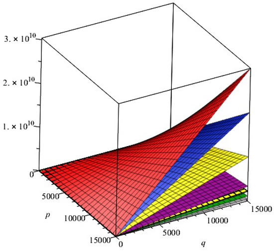
Figure 3. Comparison of indices, first and second Zagreb indexes, $ABC$ index, $GA$ index, $AB{C}_4$ index, $G{A}_5$ index, and general Randić index for $\alpha \in \{1,-1,1/2,-1/2\}$ of 2D structure of $S{i}_2{C}_3$-$I[p,q]$. $R_1$, Red; $R_{\frac{1}{2}}$, orange; $R_{-\frac{1}{2}}$, Green; $R_{-1}$,Gray; $ABC$, Cayn; $GA$,Niagara purple; $M_1$, Niagara Navy; $M_2$, off white.

Table 11 demonstrates the edge parcel in light of the degree total of end vertices of each edge of the chemical graph $S{i}_2{C}_3$-$I[p,q]$ for $p,q\ge 2$.

Table 11. Edge partition of $S{i}_2{C}_3$-$I[p,q]$.

$\left(\mathit{d}\right(\mathit{s}),\mathit{d}(\mathit{t}\left)\right)$	$({\mathit{S}}_{\mathit{u}},{\mathit{S}}_{\mathit{v}})$	Frequency
$(2,1)$	$(4,2)$	1
$(3,1)$	$(5,3)$	1
$(2,2)$	$(5,5)$	$p+2q$
$(3,2)$	$(5,5)$	1
$(3,2)$	$(7,4)$	1
$(3,2)$	$(7,5)$	$2(q+1)$
$(3,2)$	$(5,6)$	1
$(3,2)$	$(7,6)$	$4p+2q-7$
$(3,2)$	$(8,6)$	$2(q-1)$
$(3,2)$	$(8,5)$	$2p+2q-5$
$(3,3)$	$(8,7)$	1
$(3,3)$	$(8,8)$	$p+2q-4$
$(3,3)$	$(9,7)$	$2p+2q-3$
$(3,3)$	$(9,8)$	$2p+4q-7$
$(3,3)$	$(9,9)$	$15pq-14p-21q+20$

• The fourth atom–bond connectivity index $AB{C}_4\left(S{i}_2{C}_3-I[p,q]\right).$

Let G be the graph of Silicon Carbide of type $S{i}_2{C}_3$-$I[p,q]$. Now, by using Table 11, the fourth atom–bond connectivity index is computed as below (see Table 12):

$$\begin{array}{ccc}\hfill AB{C}_4\left(G\right)& =& \sum _{st\in E\left(G\right)}\sqrt{\frac{S\left(s\right)+S\left(t\right)-2}{S\left(s\right)S\left(t\right)}},\hfill \\ \hfill AB{C}_4\left(G\right)& =& \left(1\right)\sqrt{\frac{4+2-2}{4\times 2}}+\left(1\right)\sqrt{\frac{5+3-2}{5\times 3}}+(p+2q+1)\sqrt{\frac{5+5-2}{5\times 5}}\hfill \\ & +& 2(q-1)\sqrt{\frac{7+5-2}{7\times 5}}+\left(1\right)\sqrt{\frac{5+6-2}{5\times 6}}+(4p+2q-7)\sqrt{\frac{7+6-2}{7\times 6}}\hfill \\ & +& 2(q-1)\sqrt{\frac{8+6-2}{8\times 6}}+(2p+2q-5)\sqrt{\frac{8+5-2}{8\times 5}}+\left(1\right)\sqrt{\frac{7+4-2}{7\times 4}}\hfill \\ & +& \left(1\right)\sqrt{\frac{8+7-2}{8\times 7}}+(p+2q-4)\sqrt{\frac{8+8-2}{8\times 8}}+(2p+2q-3)\sqrt{\frac{9+7-2}{9\times 7}}\hfill \\ & +& (2p+4q-7)\sqrt{\frac{9+8-2}{9\times 8}}+(15pq-14p-21q+20)\sqrt{\frac{9+9-2}{9\times 9}}.\hfill \end{array}$$

Table 12. The fourth atom–bond connectivity index.

$[\mathit{p},\mathit{q}]$	$[1,1]$	$[2,2]$	$[3,3]$	$[4,4]$	$[5,5]$	$[6,6]$	$[7,7]$
$AB{C}_4\left(G\right)$	$9.42$	$32.21$	$68.26$	$106.18$	$156.24$	$214.52$	$287.32$

After an easy calculation, we get:

$$\begin{array}{ccc}\hfill AB{C}_4\left(G\right)& =& 20/3pq-\frac{56}{9}p-\frac{25}{3}q\hfill \\ & +& p\left[\frac{2\sqrt{2}}{5}+4\sqrt{\frac{11}{42}}+\sqrt{\frac{11}{10}}+\frac{\sqrt{14}}{8}+\frac{2\sqrt{2}}{3}+\frac{1}{3}\sqrt{\frac{15}{2}}\right]\hfill \\ & +& q\left[\frac{4\sqrt{2}}{5}+2\sqrt{\frac{2}{7}}+2\sqrt{\frac{11}{42}}+\sqrt{\frac{11}{10}}+\frac{\sqrt{14}}{4}+\frac{2\sqrt{2}}{3}+\frac{2}{3}\sqrt{\frac{15}{2}}\right]\hfill \\ & +& \frac{1}{\sqrt{2}}+\sqrt{\frac{2}{5}}+\frac{2\sqrt{2}}{5}-2\sqrt{\frac{2}{7}}+\frac{3}{\sqrt{30}}-7\sqrt{\frac{11}{42}}-\frac{5}{2}\sqrt{\frac{11}{10}}+\frac{3}{2}\frac{1}{\sqrt{7}}\hfill \\ & +& \frac{1}{2}\sqrt{\frac{13}{14}}-\frac{\sqrt{14}}{2}-\sqrt{2}-\frac{7}{6}\sqrt{\frac{15}{2}}+\frac{71}{9}.\hfill \end{array}$$

• The fifth geometric arithmetic index $G{A}_5\left(S{i}_2{C}_3-I[p,q]\right)$

Let G be the graph of $S{i}_2{C}_3$-$I[p,q]$. Now, by using Table 11, the fifth geometric arithmetic index is computed as below (see Table 13):

$$\begin{array}{ccc}\hfill G{A}_5\left(G\right)& =& \sum _{st\in E\left(G\right)}\frac{2\sqrt{S\left(s\right)S\left(t\right)}}{S\left(s\right)+S\left(t\right),}\hfill \end{array}$$

$$\begin{array}{ccc}\hfill G{A}_5\left(G\right)& =& \left(1\right)\frac{2\sqrt{4\times 2}}{4+2}+\left(1\right)\frac{2\sqrt{5\times 3}}{5+3}+(p+2q+1)\frac{2\sqrt{5\times 5}}{5+5}\hfill \\ & +& 2(q-1)\frac{2\sqrt{7\times 5}}{7+5}+\left(1\right)\frac{2\sqrt{5\times 6}}{5+6}+(4p+2q-7)\frac{2\sqrt{7\times 6}}{7+6}\hfill \\ & +& 2(q-1)\frac{2\sqrt{8\times 6}}{8+6}+(2p+2q-5)\frac{2\sqrt{8\times 5}}{8+5}+\left(1\right)\frac{2\sqrt{7\times 4}}{7+4}\hfill \\ & +& \left(1\right)\frac{2\sqrt{8\times 7}}{8+7}+(p+2q-4)\frac{2\sqrt{8\times 8}}{8+8}+(2p+2q-3)\frac{2\sqrt{9\times 7}}{9+7}\hfill \\ & +& (2p+4q-7)\frac{2\sqrt{9\times 8}}{9+8}+(15pq-14p-21q+20)\frac{2\sqrt{9\times 9}}{9+9},\hfill \end{array}$$

$$\begin{array}{ccc}\hfill G{A}_5\left(G\right)& =& 15pq+p\left[\frac{8}{13}\sqrt{42}+\frac{8}{13}\sqrt{10}+\frac{3}{4}\sqrt{7}+\frac{24}{17}\sqrt{2}-12\right]\hfill \\ & +& q\left[\frac{1}{3}\sqrt{35}+\frac{4}{13}\sqrt{42}+\frac{4\sqrt{12}}{7}+\frac{8}{13}\sqrt{10}+\frac{3}{4}\sqrt{7}+\frac{48}{17}\sqrt{2}-17\right]\hfill \\ & +& \frac{2\sqrt{2}}{3}+\frac{\sqrt{15}}{4}-\frac{\sqrt{35}}{3}+\frac{2\sqrt{30}}{11}-\frac{14\sqrt{42}}{13}-\frac{4\sqrt{12}}{7}-\frac{20\sqrt{10}}{13}\hfill \\ & +& \frac{4\sqrt{7}}{11}+\frac{4\sqrt{14}}{15}-\frac{9\sqrt{7}}{8}-\frac{84\sqrt{2}}{17}+17.\hfill \end{array}$$

Table 13. The fifth geometric arithmetic index.

$[\mathit{p},\mathit{q}]$	$[1,1]$	$[2,2]$	$[3,3]$	$[4,4]$	$[5,5]$	$[6,6]$	$[7,7]$
$G{A}_5\left(G\right)$	$19.26$	$69.31$	$143.28$	$251.21$	$304.25$	$360.56$	$412.32$

• Comparison of topological indices for $S{i}_2{C}_3$-$I[p,q]$

In this section, we presented the comparison of above calculated topological indices for $S{i}_2{C}_3$-$I[p,q]$ graphically in Figure 4.

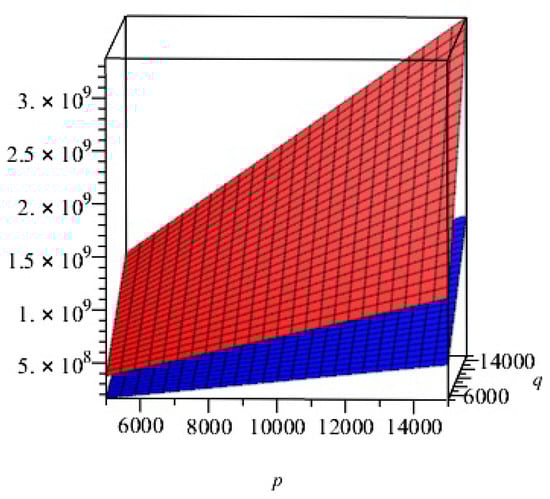
Figure 4. Comparison of $AB{C}_4$ and $G{A}_5$ indices of 2D structure of $S{i}_2{C}_3$-$I[p,q]$. Blue and red colors represents $AB{C}_4$ and $G{A}_5$, respectively.

5. Silicon Carbide $S{i}_2{C}_3$-$\mathrm{II}[p,q]$ 2D Structure

The 2D molecular graph of Silicon Carbide $S{i}_2{C}_3$-$II$ is given in Figure 5. To describe its molecular graph, we have used the settings in this way: we define p as the number of connected unit cells in a row (chain) and, by q, we represent the number of connected rows, each with p number of cells. In Figure 6, we gave a demonstration of how the cells connect in a row (chain) and how one row connects to another row. We will denote this molecular graph by $S{i}_2{C}_3$-$II[p,q]$. Thus, the quantity of vertices in this graph is $10pq$ and the number of edges are $15pq-3p-3q$.

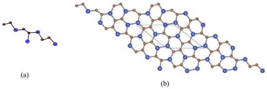
Figure 5. 2D structure of $S{i}_2{C}_3$-$II[p,q]$, (a) chemical unit cell of $S{i}_2{C}_3$-$II[p,q]$; (b) $S{i}_2{C}_3$-$II[3,3]$. Carbon atom C are brown and Silicon atom $Si$ are blue

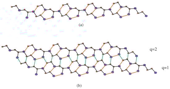
Figure 6. 2D structure of $S{i}_2{C}_3$-$II[p,q]$, (a) $S{i}_2{C}_3$-$II[5,1]$, one row with $p=5$ and $q=1$. Red lines show the connection between the unit cells; (b) $S{i}_2{C}_3$-$II[5,2]$, and two rows are connecting. Green lines (edges) connect the upper and lower rows.

5.1. Methodology of Silicon Carbide $S{i}_2{C}_3$-$II[p,q]$ Formulas

For the computation of these formulas for Silicon Carbide $S{i}_2{C}_3$-$II[p,q]$, we first use a unit cell and then combine it with another unit cell in the horizontal direction and so on up to p unit cells. After this, we use first a unit cell and then combine it with another unit cell in the vertical direction and so on up to q unit cells. Thus, we obtained Silicon Carbide $S{i}_2{C}_3$-$II[p,q]$ structure (see Figure 5). Now, for the computation of vertices, we use Table 14 and Matlab software for generalizing these formulas of vertices. In the following table, $V_1$ represents the quantity of vertices of degree 1, $V_2$ represents the quantity of vertices of degree 2 and $V_3$ represents the quantity of vertices of degree 3.

Table 14. Vertex partition of $S{i}_2{C}_3$-$II[p,q]$.

$[\mathit{p},\mathit{q}]$	$[1,1]$	$[1,2]$	$[1,3]$	$[2,1]$	$[2,2]$	$[2,3]$	$[3,1]$	$[3,2]$	$[3,3]$	$[4,1]$	$[4,2]$	$[4,3]$
$V_1$	3	3	3	3	3	3	3	3	3	3	3	3
$V_2$	6	12	18	12	18	24	18	24	30	24	30	36
$V_3$	1	5	9	5	19	33	9	33	57	13	47	81

Now, in general, the quantity of vertices of degree 1 are 3, the quantity of vertices of degree 2 are $6(p+q-1)$, the quantity of vertices of degree 3 are $10pq-6p-6q+3$.

To find the abstracted indices, we will partition the edges of $S{i}_2{C}_3$-$II[p,q]$ using the above methodology. Moreover, we use the combinatorial counting and standard edge partition. The first edge parcel contains 2 edge $st$, where $deg\left(u\right)=2$ and $d\left(t\right)=1$. The second edge parcel contains only one edge $st$, where $deg\left(u\right)=3$ and $d\left(t\right)=1$. The third edge parcel contains $2(p+q)$ edges $st$, where $deg\left(u\right)=2$ and $d\left(t\right)=2$. The fourth edge parcel contains $8p+8q-14$ number of edges $st$, where $deg\left(u\right)=3$ and $d\left(t\right)=2$. The fifth edge parcel contains $15pq-13p-13q+11$ number of edges $st$, where $deg\left(u\right)=d\left(t\right)=3$. Table 15 shows the edge partition of $S{i}_2{C}_3$-$II[p,q]$ with $p,q\ge 1$.

Table 15. Edge partition of $S{i}_2{C}_3$-$II[p,q]$.

$\left(\mathit{d}\right(\mathit{s}),\mathit{d}(\mathit{t}\left)\right)$	Frequency
$(2,1)$	2
$(3,1)$	1
$(2,2)$	$2p+2q$
$(3,2)$	$8p+8q-14$
$(3,3)$	$15pq-13p-13q+11$

5.2. Main Results for Silicon Carbide $S{i}_2{C}_3-II[p,q]$

In this section, we compute the general result of topological indices for $S{i}_2{C}_3-II[p,q]$. In addition, we construct the tables for these indices for small values of $p,q$. Moreover, we give graphical comparison and application of these indices.

• Atom–bond connectivity index $ABC(S{i}_2{C}_3$-$IO[p,q])$

Let G be the graph of Silicon Carbide of type $S{i}_2{C}_3$-$II[p,q]$. Then, from the edge partition of $S{i}_2{C}_3$-$II[p,q]$ which is given in Table 15, the atom–bond connectivity index can be calculated as (see Table 16):

$$\begin{array}{ccc}\hfill ABC\left(G\right)& =& \sum _{st\in E\left(G\right)}\sqrt{\frac{d\left(s\right)+d\left(t\right)-2}{d\left(s\right)d\left(t\right)}},\hfill \\ \hfill ABC\left(G\right)& =& \left(2\right)\sqrt{\frac{2+1-2}{2\times 1}}+\left(1\right)\sqrt{\frac{3+1-2}{3\times 1}}+(2p+2q)\sqrt{\frac{2+2-2}{2\times 2}}\hfill \\ & +& (8p+8q-14)\sqrt{\frac{3+2-2}{3\times 2}}+(15pq-13p-13q+11)\sqrt{\frac{3+3-2}{3\times 3}},\hfill \\ \hfill ABC\left(G\right)& =& 10pq+(p+q)\left[\frac{10}{\sqrt{2}}-\frac{26}{3}\right]-12\frac{1}{\sqrt{2}}+\sqrt{\frac{2}{3}}+\frac{22}{3}.\hfill \end{array}$$

Table 16. The atom–bond connectivity index.

$[\mathit{p},\mathit{q}]$	$[1,1]$	$[2,2]$	$[3,3]$	$[4,4]$	$[5,5]$	$[6,6]$	$[7,7]$
$ABC\left(G\right)$	$13.25$	$45.26$	$95.17$	$165.26$	$240.32$	$330.15$	$440.14$

• The general Randić index $R_{\alpha }(S{i}_2{C}_3$-$II[p,q])$

Let G be the graph of $S{i}_2{C}_3$-$II[p,q]$. Now, by using Table 15, the general Randić index for $\alpha =1$ (see Table 17),

$$\begin{array}{ccc}\hfill R_1\left(G\right)& =& \sum _{st\in E\left(G\right)}(d\left(s\right)\times d\left(t\right)),\hfill \\ \hfill R_1\left(G\right)& =& \left(2\right)(2\times 1)+\left(1\right)(3\times 1)+(2p+2q)(2\times 2)\hfill \\ & +& (8p+8q-14)(3\times 2)+(15pq-13p-13q+11)(3\times 3),\hfill \\ \hfill R_1\left(G\right)& =& 135pq-61p-61q+22.\hfill \end{array}$$

Table 17. The Randić index for $\alpha =1$.

$[\mathit{p},\mathit{q}]$	$[1,1]$	$[2,2]$	$[3,3]$	$[4,4]$	$[5,5]$	$[6,6]$	$[7,7]$
$R_1\left(G\right)$	35	318	871	1694	2459	4024	5714

For $\alpha =-1$ (see Table 18),

$$\begin{array}{ccc}\hfill R_{-1}\left(G\right)& =& \sum _{st\in E\left(G\right)}\frac{1}{\left(d\right(s)\times d(t\left)\right)},\hfill \\ \hfill R_{-1}\left(G\right)& =& \left(2\right)(\frac{1}{2\times 1})+\left(1\right)(\frac{1}{3\times 1})+(2p+2q)(\frac{1}{2\times 2})+(8p+8q-14)(\frac{1}{3\times 2})\hfill \\ & +& (15pq-13p-13q+11)(\frac{1}{3\times 3}),\hfill \\ \hfill R_{-1}\left(G\right)& =& \frac{5}{3}pq+\frac{7}{18}p+\frac{7}{18}q+\frac{2}{9}.\hfill \end{array}$$

Table 18. The Randić index for $\alpha =-1$.

$[\mathit{p},\mathit{q}]$	$[1,1]$	$[2,2]$	$[3,3]$	$[4,4]$	$[5,5]$	$[6,6]$	$[7,7]$
$R_{-1}\left(G\right)$	$2.10$	$9.12$	$16.28$	$28.11$	$39.12$	$50.12$	$63.41$

For $\alpha =\frac{1}{2}$ (see Table 19),

$$\begin{array}{ccc}\hfill R_{\frac{1}{2}}\left(G\right)& =& \sum _{st\in E\left(G\right)}\sqrt{\left(d\right(s)\times d(t\left)\right)},\hfill \\ \hfill R_{\frac{1}{2}}\left(G\right)& =& \left(2\right)\left(\sqrt{2\times 1}\right)+\left(1\right)\left(\sqrt{3\times 1}\right)+(2p+2q)\left(\sqrt{2\times 2}\right)\hfill \\ & +& (8p+8q-14)\left(\sqrt{3\times 2}\right)+(15pq-13p-13q+11)\left(\sqrt{3\times 3}\right),\hfill \\ \hfill R_{\frac{1}{2}}\left(G\right)& =& 45pq+(p+q)\left[8\sqrt{6}-35\right]+2\sqrt{2}+\sqrt{3}-14\sqrt{6}+33.\hfill \end{array}$$

Table 19. The Randić index for $\alpha =\frac{1}{2}$.

$[\mathit{p},\mathit{q}]$	$[1,1]$	$[2,2]$	$[3,3]$	$[4,4]$	$[5,5]$	$[6,6]$	$[7,7]$
$R_{\frac{1}{2}}\left(G\right)$	$48.32$	$58.23$	$79.11$	$95.21$	$115.23$	$135.25$	$160.13$

For $\alpha =\frac{-1}{2}$ (see Table 20),

$$\begin{array}{ccc}\hfill R_{-\frac{1}{2}}\left(G\right)& =& \sum _{st\in E\left(G\right)}\frac{1}{\sqrt{\left(d\right(s)\times d(t\left)\right)}},\hfill \\ \hfill R_{-\frac{1}{2}}\left(G\right)& =& \left(2\right)(\frac{1}{\sqrt{2\times 1}})+\left(1\right)(\frac{1}{\sqrt{3\times 1}})+(2p+2q)(\frac{1}{\sqrt{2\times 2}})\hfill \\ & +& (8p+8q-14)(\frac{1}{\sqrt{3\times 2}})+(15pq-13p-13q+11)(\frac{1}{\sqrt{3\times 3}}),\hfill \\ \hfill R_{-\frac{1}{2}}\left(G\right)& =& 5pq+(p+q)\left[\frac{8}{\sqrt{6}}-\frac{10}{3}\right]+\sqrt{2}+\frac{1}{\sqrt{3}}-\frac{14}{\sqrt{6}}+\frac{11}{3}.\hfill \end{array}$$

Table 20. The Randić index for $\alpha =\frac{-1}{2}$.

$[\mathit{p},\mathit{q}]$	$[1,1]$	$[2,2]$	$[3,3]$	$[4,4]$	$[5,5]$	$[6,6]$	$[7,7]$
$R_{\frac{-1}{2}}\left(G\right)$	$6.21$	$23.51$	$48.25$	$84.36$	$108.32$	$133.42$	$168.24$

• The geometric arithmetic index $GA(S{i}_2{C}_3$-$II[p,q])$

Let G be the graph of Silicon Carbide $S{i}_2{C}_3$-$II[p,q]$. Now, by using Table 15, the geometric arithmetic index is computed as below (see Table 21):

$$\begin{array}{ccc}\hfill GA\left(G\right)& =& \sum _{st\in E\left(G\right)}\frac{2\sqrt{d\left(s\right)d\left(t\right)}}{d\left(s\right)+d\left(t\right)},\hfill \\ \hfill GA\left(G\right)& =& \left(2\right)\frac{2\sqrt{2}}{2+1}+\left(1\right)\frac{2\sqrt{3}}{3+1}+(2p+2q)\frac{2\sqrt{4}}{2+2}+(8p+8q-14)\frac{2\sqrt{6}}{3+2}\hfill \\ & +& (15pq-13p-13q+11)\frac{2\sqrt{9}}{3+3},\hfill \\ \hfill GA\left(G\right)& =& 15pq+(p+q)\left[\frac{16\sqrt{6}}{5}-11\right]+\frac{4\sqrt{2}}{3}+\frac{\sqrt{3}}{2}-\frac{28\sqrt{6}}{5}+11.\hfill \end{array}$$

Table 21. The geometric arithmetic index.

$[\mathit{p},\mathit{q}]$	$[1,1]$	$[2,2]$	$[3,3]$	$[4,4]$	$[5,5]$	$[6,6]$	$[7,7]$
$GA\left(G\right)$	$18.35$	$64.21$	$135.11$	$236.42$	$346.12$	$460.25$	$580.12$

• The first and second Zagreb index

Let G be the graph of $S{i}_2{C}_3$-$II[p,q]$. Now, by using Table 15, the first Zagreb index is computed as below (see Table 22):

$$\begin{array}{ccc}\hfill M_1\left(G\right)& =& \sum _{st\in E\left(G\right)}(d\left(s\right)+d\left(t\right)),\hfill \\ \hfill M_1\left(G\right)& =& \left(2\right)(2+1)+\left(1\right)(3+1)+(2p+2q)(2+2)+(8p+8q-14)(3+2)\hfill \\ & +& (15pq-13p-13q+11)(3+3),\hfill \\ \hfill M_1\left(G\right)& =& 90pq-30p-30q+6.\hfill \end{array}$$

Table 22. The first Zagreb index.

$[\mathit{p},\mathit{q}]$	$[1,1]$	$[2,2]$	$[3,3]$	$[4,4]$	$[5,5]$	$[6,6]$	$[7,7]$
$M_1\left(G\right)$	36	246	636	1206	1836	3244	4634

The second Zagreb index is computed below (see Table 23):

$$\begin{array}{ccc}\hfill M_2\left(G\right)& =& \sum _{st\in E\left(G\right)}\left(d\left(s\right)d\left(t\right)\right)=R_1\left(G\right),\hfill \\ \hfill M_2\left(G\right)& =& \left(2\right)(2\times 1)+\left(1\right)(3\times 1)+(2p+2q)(2\times 2)+(8p+8q-14)(3\times 2)\hfill \\ & +& (15pq-13p-13q+11)(3\times 3),\hfill \\ \hfill M_2\left(G\right)& =& 135pq-61p-61q+22.\hfill \end{array}$$

Table 23. The second Zagreb index.

$[\mathit{p},\mathit{q}]$	$[1,1]$	$[2,2]$	$[3,3]$	$[4,4]$	$[5,5]$	$[6,6]$	$[7,7]$
$M_2\left(G\right)$	35	318	871	1694	2654	4064	6248

• Comparison of topological indices for $S{i}_2{C}_3-II[p,q]$

In this section, we presented the comparison of above calculated topological indices for $S{i}_2{C}_3-II[p,q]$ graphically in Figure 7.

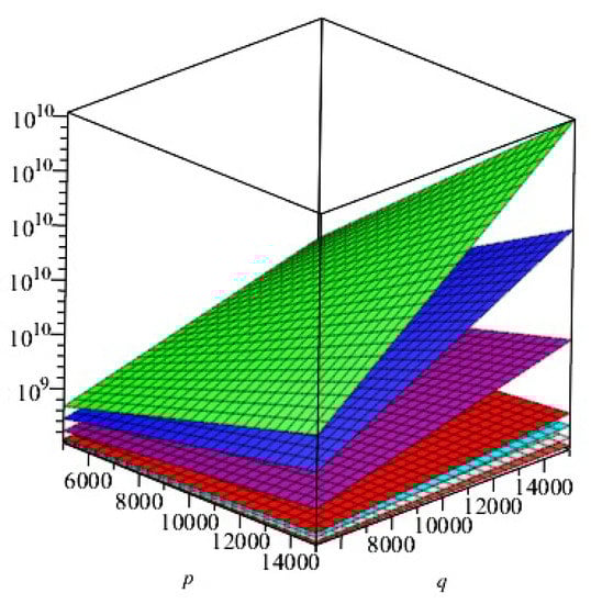
Figure 7. Comparison of indices, first and second Zagreb indexes, $ABC$ index, $GA$ index, $AB{C}_4$ index, $G{A}_5$ index, and general Randić index for $\alpha \in \{1,-1,1/2,-1/2\}$ of 2D structure of $S{i}_2{C}_3$-$II[p,q]$. $R_1$,Green; $R_{\frac{1}{2}}$, Purple; $R_{-\frac{1}{2}}$, Gray; $R_{-1}$,Orange; $ABC$, Cayn; $GA$,Red; $M_1$, Blue; $M_2$, yellow.

Table 24 demonstrates the edge parcel in light of the degree total of end vertices of each edge of the chemical graph $S{i}_2{C}_3$-$II[p,q]$ for $p,q\ge 2$.

Table 24. Edge partition of $S{i}_2{C}_3$-$II[p,q]$.

$\left(\mathit{d}\right(\mathit{s}),\mathit{d}(\mathit{t}\left)\right)$	$({\mathit{S}}_{\mathit{u}},{\mathit{S}}_{\mathit{v}})$	Frequency
$(2,1)$	$(3,2)$	2
$(3,1)$	$(7,3)$	1
$(2,2)$	$(4,3)$	2
$(2,2)$	$(5,4)$	2
$(2,2)$	$(5,5)$	$2p+2q-4$
$(3,2)$	$(7,5)$	$2p+2q$
$(3,2)$	$(7,6)$	$2p+2q-2$
$(3,2)$	$(8,6)$	$2p+2q-6$
$(3,2)$	$(8,5)$	$2p+2q-6$
$(3,3)$	$(8,7)$	2
$(3,3)$	$(8,8)$	$2(p+q-4)$
$(3,3)$	$(7,7)$	2
$(3,3)$	$(9,7)$	$2p+2q-3$
$(3,3)$	$(9,8)$	$2p+2q-5$
$(3,3)$	$(9,9)$	$15pq-19p-19q+23$

• The fourth atom–bond connectivity index $AB{C}_4\left(S{i}_2{C}_3-II[p,q]\right)$

Let G be the graph of Silicon Carbide of type $S{i}_2{C}_3$-$II[p,q]$. Now, by using Table 24, the fourth atom–bond connectivity index is computed as (see Table 25):

$$\begin{array}{ccc}\hfill AB{C}_4\left(G\right)& =& \sum _{st\in E\left(G\right)}\sqrt{\frac{S\left(s\right)+S\left(t\right)-2}{S\left(s\right)S\left(t\right)}},\hfill \\ \hfill AB{C}_4\left(G\right)& =& \left(2\right)\sqrt{\frac{3+2-2}{3\times 2}}+\left(1\right)\sqrt{\frac{7+3-2}{7\times 3}}+\left(2\right)\sqrt{\frac{4+3-2}{4\times 3}}+\left(2\right)\sqrt{\frac{5+4-2}{5\times 4}}\hfill \\ & +& (2p+2q-4)\sqrt{\frac{5+5-2}{5\times 5}}+(2p+2q)\sqrt{\frac{7+5-2}{7\times 5}}+2(p+q-1)\sqrt{\frac{7+6-2}{7\times 6}}\hfill \\ & +& (2p+2q-6)\sqrt{\frac{8+6-2}{8\times 6}}+(2p+2q-6)\sqrt{\frac{8+5-2}{8\times 5}}+\left(2\right)\sqrt{\frac{8+7-2}{8\times 7}}\hfill \\ & +& 2(p+q-4)\sqrt{\frac{8+8-2}{8\times 8}}+\left(2\right)\sqrt{\frac{7+7-2}{7\times 7}}+(2p+2q-3)\sqrt{\frac{9+7-2}{9\times 7}}\hfill \\ & +& (2p+2q-5)\sqrt{\frac{9+8-2}{9\times 8}}+(15pq-19p-19q+23)\sqrt{\frac{9+9-2}{9\times 9}}.\hfill \end{array}$$

Table 25. The fourth atom–bond connectivity index.

$[\mathit{p},\mathit{q}]$	$[1,1]$	$[2,2]$	$[3,3]$	$[4,4]$	$[5,5]$	$[6,6]$	$[7,7]$
$AB{C}_4\left(G\right)$	$7.21$	$28.23$	$64.11$	$101.21$	$142.28$	$208.44$	$266.64$

After an easy calculation, we get:

$$\begin{array}{ccc}\hfill AB{C}_4\left(G\right)& =& \frac{20}{3}pq\hfill \\ & +& (p+q)\left[\frac{22\sqrt{2}}{15}+2\sqrt{\frac{2}{7}}+2\sqrt{\frac{11}{42}}+\sqrt{\frac{11}{10}}+\frac{\sqrt{14}}{4}+\frac{1}{3}\sqrt{\frac{15}{2}}-67/9\right]\hfill \\ & +& \sqrt{2}+2\sqrt{\frac{2}{21}}+\frac{2}{5}\sqrt{\frac{5}{3}}+\sqrt{\frac{7}{5}}-\frac{13\sqrt{2}}{5}-2\sqrt{\frac{11}{42}}-3\sqrt{\frac{11}{10}}\hfill \\ & +& \sqrt{\frac{13}{14}}-\sqrt{14}+\frac{4\sqrt{3}}{7}-\frac{5}{6}\sqrt{\frac{15}{2}}+\frac{65}{9}.\hfill \end{array}$$

• The fifth geometric arithmetic index $G{A}_5\left(S{i}_2{C}_3-II[p,q]\right)$

Let G be the graph of $S{i}_2{C}_3$-$II[p,q]$. Now, by using Table 24, the fifth geometric arithmetic index is computed as (see Table 26):

$$\begin{array}{ccc}\hfill G{A}_5\left(G\right)& =& \sum _{st\in E\left(G\right)}\frac{2\sqrt{S\left(s\right)S\left(t\right)}}{S\left(s\right)+S\left(t\right)},\hfill \\ \hfill G{A}_5\left(G\right)& =& \left(2\right)\frac{2\sqrt{3\times 2}}{3+2}+\left(1\right)\frac{2\sqrt{7\times 3}}{7+3}+\left(2\right)\frac{2\sqrt{4\times 3}}{4+3}+\left(2\right)\frac{2\sqrt{5\times 4}}{5+4}\hfill \\ & +& (2p+2q-4)\frac{2\sqrt{5\times 5}}{5+5}+(2p+2q)\frac{2\sqrt{7\times 5}}{7+5}+2(p+q-1)\frac{2\sqrt{7\times 6}}{7+6}\hfill \\ & +& (2p+2q-6)\frac{2\sqrt{8\times 6}}{8+6}+(2p+2q-6)\frac{2\sqrt{8\times 5}}{8+5}+\left(2\right)\frac{2\sqrt{8\times 7}}{8+7}\hfill \\ & +& 2(p+q-4)\frac{2\sqrt{8\times 8}}{8+8}+\left(2\right)\frac{2\sqrt{7\times 7}}{7+7}+(2p+2q-3)\frac{2\sqrt{9\times 7}}{9+7}\hfill \\ & +& (2p+2q-5)\frac{2\sqrt{9\times 8}}{9+8}+(15pq-19p-19q+23)\frac{2\sqrt{9\times 9}}{9+9},\hfill \\ \hfill G{A}_5\left(G\right)& =& 15pq+(p+q)\left[\frac{\sqrt{35}}{3}+\frac{4\sqrt{42}}{13}+\frac{8\sqrt{3}}{7}+\frac{8\sqrt{10}}{13}+\frac{3\sqrt{7}}{4}+\frac{24\sqrt{2}}{17}-15\right]\hfill \\ & +& \frac{4\sqrt{6}}{5}+\frac{\sqrt{21}}{5}+\frac{8\sqrt{3}}{7}+\frac{8\sqrt{5}}{9}-\frac{4\sqrt{42}}{13}-\frac{24\sqrt{3}}{7}-\frac{24\sqrt{10}}{13}+\frac{8\sqrt{14}}{15}\hfill \\ & -& \frac{9\sqrt{7}}{8}-\frac{60\sqrt{2}}{17}+13.\hfill \end{array}$$

Table 26. The fifth geometric arithmetic index.

$[\mathit{p},\mathit{q}]$	$[1,1]$	$[2,2]$	$[3,3]$	$[4,4]$	$[5,5]$	$[6,6]$	$[7,7]$
$G{A}_5\left(G\right)$	$17.12$	$64.34$	$139.18$	$246.42$	$298.24$	$354.54$	$408.44$

• Comparison of topological indices for $S{i}_2{C}_3$-$II[p,q]$

We presented the comparison of topological indices for $S{i}_2{C}_3$-$II[p,q]$ graphically in Figure 8.

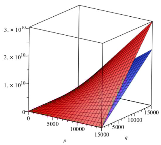
Figure 8. Comparison of $AB{C}_4$ and $G{A}_5$ indices of 2D structure of $S{i}_2{C}_3$-$II[p,q]$. Blue and red colors represents $AB{C}_4$ and $G{A}_5$, respectively.

6. Comparisons and Discussion

In this section, we have computed all indices for different values of $p,q$ for both structures $S{i}_2{C}_3$-$I[p,q]$ and $S{i}_2{C}_3$-$II[p,q]$. In addition, we construct Table 3, Table 4, Table 5, Table 6, Table 7, Table 8, Table 9, Table 10, Table 12 and Table 13 for small values of $p,q$ for these topological indices to the structure $S{i}_2{C}_3$-$I[p,q]$ and Table 16, Table 17, Table 18, Table 19, Table 20, Table 21, Table 22, Table 23, Table 25 and Table 26 to the structure $S{i}_2{C}_3$-$II[p,q]$. Now, from Table 27 and Table 28, we can easily see that all indices are in increasing order as the values of $p,q$ are increases. In addition, on the other hand, indices showed higher values for $S{i}_2{C}_3$-$I[p,q],$ as compared to those of $S{i}_2{C}_3$-$II[p,q]$.

Table 27. Comparison of all indices for $S{i}_2{C}_3$-$I[p,q]$.

$[\mathit{p},\mathit{q}]$	$\mathit{ABC}$	${\mathit{R}}_1$	${\mathit{R}}_{-1}$	${\mathit{R}}_{\frac{1}{2}}$	${\mathit{R}}_{\frac{-1}{2}}$	$\mathit{GA}$	${\mathit{M}}_1$	${\mathit{M}}_2$	${\mathit{ABC}}_4$	${\mathit{GA}}_5$
$[1,1]$	$16.2$	77	$2.41$	$49.31$	$7.42$	$19.25$	44	47	$9.42$	$19.26$
$[2,2]$	$48.3$	350	$11.32$	$60.34$	$25.18$	$68.29$	264	350	$32.21$	$69.31$
$[3,3]$	$98.7$	923	$18.11$	$80.41$	$51.23$	$141.12$	664	923	$68.26$	$143.28$
$[4,4]$	$169.3$	1766	$29.12$	$97.11$	$87.04$	$248.41$	1244	1766	$106.18$	$251.21$

Table 28. Comparison of all indices for $S{i}_2{C}_3$-$II[p,q]$.

$[\mathit{p},\mathit{q}]$	$\mathit{ABC}$	${\mathit{R}}_1$	${\mathit{R}}_{-1}$	${\mathit{R}}_{\frac{1}{2}}$	${\mathit{R}}_{\frac{-1}{2}}$	$\mathit{GA}$	${\mathit{M}}_1$	${\mathit{M}}_2$	${\mathit{ABC}}_4$	${\mathit{GA}}_5$
$[1,1]$	$13.25$	35	$2.10$	$48.32$	$6.21$	$18.35$	36	35	$7.21$	$17.12$
$[2,2]$	$45.26$	318	$9.12$	$58.23$	$23.51$	$64.21$	246	318	$28.23$	$64.34$
$[3,3]$	$95.17$	871	$16.28$	$79.11$	$48.25$	$135.11$	636	871	$64.11$	$139.18$
$[4,4]$	$165.26$	1694	$28.11$	$95.21$	$84.39$	$236.42$	1206	1694	$101.21$	$246.42$

The graphical representations of topological indices of $S{i}_2{C}_3$-$I[p,q]$ and $S{i}_2{C}_3$-$II[p,q]$ are depicted in Figure 3, Figure 4, Figure 7 and Figure 8 for certain values of $p,q$.

Now, we presented the comparison of all topological indices using Table 27, for $S{i}_2{C}_3$-$I[p,q]$ in Figure 9 and using Table 28, for $S{i}_2{C}_3$-$II[p,q]$ in Figure 10.

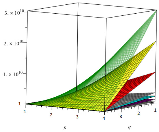
Figure 9. The comparison of all topological indices for $S{i}_2{C}_3$-$I[p,q]$.

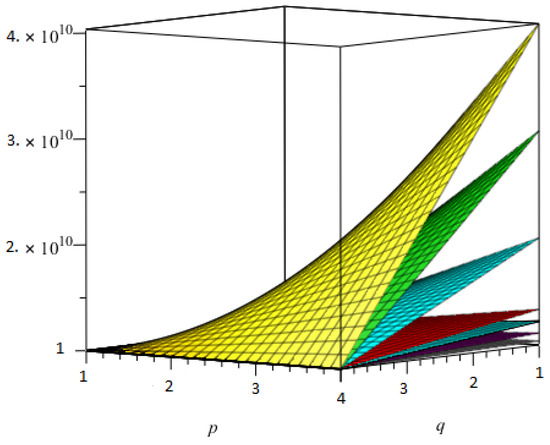
Figure 10. The comparison of all topological indices for $S{i}_2{C}_3$-$II[p,q]$.

7. Conclusions

We have studied and computed additive degree based topological indices, mainly atom–bond connectivity $ABC$ index, general Randić index, first and second Zagreb index, geometric arithmetic $GA$ index, fourth atom–bond connectivity $AB{C}_4$ index and fifth geometric arithmetic $G{A}_5$ index of two types of 2D Silicon Carbide, namely $S{i}_2{C}_3$-$I[p,q]$ and $S{i}_2{C}_3$-$II[p,q]$.

Since the Randic index is a topological descriptor that has correlated with a lot of chemical characteristics of the molecules. Thus, it has been found that the boiling point of $S{i}_2{C}_3$-$I[p,q]$ and $S{i}_2{C}_3$-$II[p,q]$-$I[p,q]$ is varying in increasing order for $\alpha \in \{1,-1,1/2,-1/2\}$.

Since the atom-bond connectivity $\left(ABC\right)$ index provides a very good correlation for computing the strain energy of molecules, one can easily be seen that the strain energy of $S{i}_2{C}_3$-$I[p,q]$ and $S{i}_2{C}_3$-$II[p,q]$-$I[p,q]$ is high as the values of $p,q$ increases.

In addition, $GA$ index has much better predictive power than the predictive power of the Randic index, so the $GA$ index is more useful than the Randic index for $\alpha \in \{-1,-1/2\}$ as compared to the Randic index for $\alpha \in \{1,1/2\}$ in the case of $S{i}_2{C}_3$-$I[p,q]$ and $S{i}_2{C}_3$-$II[p,q]$-$I[p,q]$.

Since the first and second Zagreb indexes were found to occur for computation of the total $\pi$-electron energy of the molecules, in the case of $S{i}_2{C}_3$-$I[p,q]$ and $S{i}_2{C}_3$-$II[p,q]$-$I[p,q]$, their values provide total $\pi$-electron energy in increasing order for higher values of $p,q$.

However, computing the distance based and counting related topological indices for these symmetrical chemical structures still remain open for investigation and as a challenge for researchers.

References

- Li, P.; Zhou, R.; Zeng, X.C. The search for the most stable structures of silicon–carbon monolayer compounds. Nanoscale 2014, 6, 1168–1175. [Google Scholar] [CrossRef] [PubMed]
- Novoselov, K.S.; Geim, A.K.; Morozov, S.V.; Jiang, D.; Zhang, D.Y.; Dubonos, S.V.; Grigorieva, I.V.; Firsov, A.A. Electric field effect in atomically thin carbon films. Science 2004, 306, 666–675. [Google Scholar] [CrossRef] [PubMed]
- Novoselov, K.S.; Mccann, E.; Morozov, S.V.; Falko, V.I.; Katsnelson, M.I.; Zeitler, U.; Jiang, D.; Schedin, F.; Geim, A.K. Unconventional quantum Hall effect and Berry’s phase of 2pi in bilayer graphene. Nat. Phys. 2006, 2, 177–187. [Google Scholar] [CrossRef]
- Li, Y.; Li, F.; Zhou, Z.; Chen, Z. Highly Stable Chiral (A)6–B Supramolecular Copolymer. A Multivalency-Based Self-Assembly Process. J. Am. Chem. Soc. 2011, 133, 900–908. [Google Scholar] [CrossRef] [PubMed]
- Zhou, L.; Zhang, Y.; Wu, L. SiC2 Siligraphene and Nanotube. Novel Donor Materials in Excitonic Solar Cells. Nano Lett. 2013, 13, 5431–5436. [Google Scholar] [CrossRef] [PubMed]
- Harris, J.M.; Hirst, J.L.; Mossinghoff, M.J. Combinatorics and Graph Theory; Springer Science and Business Media: Berlin/Heidelberg, Germany, 2008. [Google Scholar]
- Randić, M. On characterization of molecular branching. J. Am. Chem. Soc. 1975, 97, 6609–6615. [Google Scholar] [CrossRef]
- Bollobás, B.; Erdös, P. Graphs of extremal weights. Ars Combinatoria 1998, 50, 225–233. [Google Scholar] [CrossRef]
- Amic, D.; Beslo, D.; Lucic, B.; Nikolic, S.; Trinajstić, N. The vertex-connectivity index revisited. J. Chem. Inf. Comput. Sci. 1998, 38, 819–822. [Google Scholar] [CrossRef]
- Hu, Y.; Li, X.; Shi, Y.; Xu, T.; Gutman, I. On molecular graphs with smallest and greatest zeroth-order general Randić index. MATCH Commun. Math. Comput. Chem. 2005, 54, 425–434. [Google Scholar]
- Li, X.; Gutman, I. Mathematical Aspects of Randić Type Molecular Structure Descriptors; Mathematical Chemistry Monographs, No. 1; University of Kragujevac: Kragujevac, Serbia, 2006. [Google Scholar]
- Siddiqui, M.K.; Imran, M.; Ahmad, A. On Zagreb indices, Zagreb polynomials of some nanostar dendrimers. Appl. Math. Comput. 2016, 280, 132–139. [Google Scholar] [CrossRef]
- Siddiqui, M.K.; Naeem, M.; Rahman, N.A.; Imran, M. Computing topological indicesof certain networks. J. Optoelectron. Adv. Mater. 2016, 18, 884–892. [Google Scholar]
- Estrada, E.; Torres, L.; Rodríguez, L.; Gutman, I. An atom-bond connectivity inde. Modelling the enthalpy of formation of alkanes. Indian J. Chem. 1998, 37A, 849–855. [Google Scholar]
- Vukicevic, D.; Furtula, B. Topological index based on the ratios of geometrical and arithmetical means of end-vertex degrees of edges. J. Math. Chem. 2009, 46, 1369–1376. [Google Scholar] [CrossRef]
- Gutman, I.; Das, K.C. The first Zagreb index 30 years after. MATCH Commun. Math. Comput. Chem. 2004, 50, 83–92. [Google Scholar]
- Gutman, I.; Trinajstć, N. Graph theory and molecular orbitals, Total π-electron energy of alternant hydrocarbons. Chem. Phys. Lett. 1972, 17, 535–538. [Google Scholar] [CrossRef]
- Gao, W.; Wang, W.; Farahani, M.R. Topological Indices Study of Molecular Structure in Anticancer Drugs. J. Chem. 2016, 10. [Google Scholar] [CrossRef]
- Gao, W.; Imran, M.; Baig, A.Q.; Ali, H.; Farahani, M.R. Computing topological indices of Sudoku graphs. J. Appl. Math. Comput. 2017, 55, 99–117. [Google Scholar] [CrossRef]
- Gao, W.; Siddiqui, M.K.; Naeem, M.; Rehman, N.A. Topological Characterization of Carbon Graphite and Crystal Cubic Carbon Structures. Molecules 2017, 22, 1496–1507. [Google Scholar] [CrossRef] [PubMed]
- Ghorbani, A.; Hosseinzadeh, M.A. Computing ABC4 index of nanostar dendrimers. Optoelectron. Adv. Mater. Rapid Commun. 2010, 4, 1419–1422. [Google Scholar]
- Hayat, S.; Imran, M. Computation of certain topological indices of nanotubes covered by C5 and C7. J. Comput. Theor. Nanosci. 2015, 12, 533–541. [Google Scholar] [CrossRef]
- Rajan, B.; William, M.A.; Grigorious, A.C.; Stephen, S. On Certain Topological Indices of Silicate, Honeycomb and Hexagonal Networks. J. Comput. Math. Sci. 2012, 3, 530–535. [Google Scholar]
- Rostray, D.H. The modeling of chemical phenomena using topological indices. J. Comput. Chem. 1987, 8, 470–480. [Google Scholar]
- Baig, A.Q.; Imran, M.; Khalid, W.; Naeem, M. Molecular description of carbon graphite and crystal cubic carbon structures. Can. J. Chem. 2017, 95, 674–686. [Google Scholar] [CrossRef]
- Graovac, A.; Ghorbani, M.; Hosseinzadeh, M.A. Computing fifth geometric–arithmetic index for nanostar dendrimers. J. Math. Nanosci. 2011, 1, 33–42. [Google Scholar]
- Das, K.C.; Gutman, I.; Furtula, B. Survey on geometric-arithmetic indices of graphs. MATCH Commun. Math. Comput. Chem. 2011, 65, 595–644. [Google Scholar]
- Gutman, I.; Ruščić, B.; Trinajstić, N.; Wilcox, C.F. Graph theory and molecular orbitals, XII. Acyclic polyenes. J. Chem. Phys. 1975, 62, 3399–3405. [Google Scholar]
© 2018 by the authors. Licensee MDPI, Basel, Switzerland. This article is an open access article distributed under the terms and conditions of the Creative Commons Attribution (CC BY) license (http://creativecommons.org/licenses/by/4.0/).