Integrated Hybrid Second Order Algorithm for Orthogonal Projection onto a Planar Implicit Curve

Abstract

The computation of the minimum distance between a point and a planar implicit curve is a very important problem in geometric modeling and graphics. An integrated hybrid second order algorithm to facilitate the computation is presented. The proofs indicate that the convergence of the algorithm is independent of the initial value and demonstrate that its convergence order is up to two. Some numerical examples further confirm that the algorithm is more robust and efficient than the existing methods.

1. Introduction

Due to its great properties, the implicit curve has many applications. As a result, how to render implicit curves and surfaces is an important topic in computer graphics [1], which usually adopts four techniques: (1) representation conversion; (2) curve tracking; (3) space subdivision; and (4) symbolic computation. Using approximate distance tests to replace the Euclidean distance test, a practical rendering algorithm is proposed to rasterize algebraic curves in [2]. Employing the idea that field functions can be combined both on their values and gradients, a set of binary composition operators is developed to tackle four major problems in constructive modeling in [3]. As a powerful tool for implicit shape modeling, a new type of bivariate spline function is applied in [4], and it can be created from any given set of 2D polygons that divides the 2D plane into any required degree of smoothness. Furthermore, the spline basis functions created by the proposed procedure are piecewise polynomials and explicit in an analytical form.

Aside from rendering of computer graphics, implicit curves also play an important role in other aspects of computer graphics. To facilitate applications, it is important to compute the intersection of parametric and algebraic curves. Elimination theory and matrix determinant expression of the resultant in the intersection equations are used in [5]. Some researchers try to transform the problem of intersection into that of computing the eigenvalues and eigenvectors of a numeric matrix. Similar to elimination theory and matrix determinant expression, combining the marching methods with the algebraic formulation generates an efficient algorithm to compute the intersection of algebraic and NURBSsurfaces in [6]. For the cases with a degenerate intersection of two quadric surfaces, which are frequently applied in geometric and solid modeling, a simple method is proposed to determine the conic types without actually computing the intersection and to enumerate all possible conic types in [7]. M.Aizenshtein et al. [8] present a solver to robustly solve well-constrained $n\times n$ transcendental systems, which applies to curve-curve, curve-surface intersections, ray-trap and geometric constraint problems.

To improve implicit modeling, many techniques have been developed to compute the distance between a point and an implicit curve or surface. In order to compute the bounded Hausdorff distance between two real space algebraic curves, a theoretical result can reduce the bound of the Hausdorff distance of algebraic curves from the spatial to the planar case in [9]. Ron [10] discusses and analyzes formulas to calculate the curvature of implicit planar curves, the curvature and torsion of implicit space curves and the mean and Gaussian curvature for implicit surfaces, as well as curvature formulas to higher dimensions. Using parametric approximation of an implicit curve or surface, Thomas et al. [11] introduce a relatively small number of low-degree curve segments or surface patches to approximate an implicit curve or surface accurately and further constructs monoid curves and surfaces after eliminating the undesirable singularities and the undesirable branches normally associated with implicit representation. Slightly different from ref. [11], Eva et al. [12] use support function representation to identify and approximate monotonous segments of algebraic curves. Anderson et al. [13] present an efficient and robust algorithm to compute the foot points for planar implicit curves.

Contribution: An integrated hybrid second order algorithm is presented for orthogonal projection onto planar implicit curves. For any test point p, any planar implicit curve with or without singular points and any order of the planar implicit curve, any distance between the test point and the planar implicit curve, the algorithm could be convergent. It consists of two parts: the hybrid second order algorithm and the initial iterative value estimation algorithm.

The hybrid second order algorithm fuses the three basic ideas: (1) the tangent line orthogonal iteration method with one correction; (2) the steepest descent method to force the iteration point to fall on the planar implicit curve as much as it can; (3) Newton–Raphson’s iterative method to accelerate iteration.

Therefore, the hybrid second order algorithm is composed of six steps. The first step uses the steepest descent method of Newton’s iterative method to force the iterative value of the initial value to lie on the planar implicit curve, which is not associated with the test point p. In the second step, Newton’s iterative method employs the relationship determined by the test point p to accelerate the iteration process. The third step finds the orthogonal projection point q on the tangent line, which goes through the initial iterative point, of a test point p. The fourth step gets the linear orthogonal increment value. The same relationship in the second step is used once more to accelerate the iteration process in the fifth step. The final step gives some correction to the result of the iterative value in the fourth and fifth step.

One problem for the hybrid second order algorithm is that it appears divergent if the test point p lies particularly far away from the planar implicit curve. Since it has been found that when the initial iterative point is close to the orthogonal projection point ${\mathrm{p}}_{\Gamma }$, no matter how far away the test point p is from the planar implicit curve, it will be convergent, an algorithm, named the initial iterative value estimation algorithm, is proposed to drive the initial iterative value toward the orthogonal projection point ${\mathrm{p}}_{\Gamma }$ as much as possible. Accordingly, the second order algorithm with the initial iterative value estimation algorithm is named as the integrated hybrid second order algorithm.

The rest of this paper is organized as follows. Section 2 presents related work for orthogonal projection onto the planar implicit curve. Section 3 presents the integrated hybrid second order algorithm for orthogonal projection onto the planar implicit curve. In Section 4, convergent analysis for the integrated hybrid second order algorithm is described. The experimental results including the evaluation of performance data are given in Section 5. Finally, Section 6 and Section 7 conclude the paper.

2. Related Work

The existing methods can be divided into three categories: local methods, global methods and compromise methods between local and global methods.

2.1. Local Methods

The first one is Newton’s iterative method. Let point $\mathrm{x}=(x,y)$ be on a plane, and let $\Gamma :f(\mathrm{x})=0$ be a smooth planar implicit curve; its specific form can be represented as:

$$f(x,y)=0.$$

(1)

Let $\mathrm{p}=(p_1,p_2)$ be a point in the vicinity of curve $\Gamma$. The orthogonal projection point ${\mathrm{p}}_{\Gamma }$ satisfies the relationships:

$$\left\{\begin{array}{c}f\left({\mathrm{p}}_{\Gamma }\right)=0,\hfill \\ \nabla f\left({\mathrm{p}}_{\Gamma }\right)\wedge (\mathrm{p}-{\mathrm{p}}_{\Gamma })=0,\hfill \end{array}\right.$$

(2)

where ∧ is the difference-product ([14]). The nonlinear system (2) can be solved using Newton’s iterative method [15]:

$${\mathrm{x}}_{m+1}={\mathrm{x}}_m-{\mathrm{J}}^{-1}{(\mathrm{x}}_m)\mathrm{L}\left({\mathrm{x}}_m\right),$$

(3)

where $\mathrm{L}\left(\mathrm{x}\right)=\left\{\begin{array}{c}f\left(\mathrm{x}\right),\hfill \\ \nabla f\left(\mathrm{x}\right)\wedge (\mathrm{p}-\mathrm{x})\hfill \end{array}\right.$, $\mathrm{J}\left(\mathrm{x}\right)$ is the Jacobian matrix of partial derivatives of $\mathrm{L}\left(\mathrm{x}\right)$ with respect to x. Sullivan et al. [16] used Lagrange multipliers and Newton’s algorithm to compute the closest point on the curve for each point.

$$\left(\begin{array}{ccc}2+\lambda \frac{{\partial }^{2}f}{\partial x^2}& \lambda \frac{{\partial }^{2}f}{\partial x\partial y}& \frac{\partial f}{\partial x}\\ \lambda \frac{{\partial }^{2}f}{\partial x\partial y}& 2+\lambda \frac{{\partial }^{2}f}{\partial y^2}& \frac{\partial f}{\partial y}\\ \frac{\partial f}{\partial x}& \frac{\partial f}{\partial y}& 0\end{array}\right)\left(\begin{array}{c}\delta x\hfill \\ \delta y\hfill \\ \delta \lambda \hfill \end{array}\right)=-\left(\begin{array}{c}-2(p_1-x)+\lambda \frac{\partial f}{\partial x}\hfill \\ -2(p_2-y)+\lambda \frac{\partial f}{\partial y}\hfill \\ f(x,y)\hfill \end{array}\right),$$

(4)

where $\lambda$ is the Lagrange multiplier. It will converge after repeated iteration of Equation (4) for increment $\delta x,\delta y,\delta \lambda$ with the initial iterative point and $\lambda =0$. However, Newton’s iterative method or Newton-type’s iterative method is of local convergence, i.e., it sometimes failed to converge even with a reasonably good initial guess. On the other hand, once a good initial guess lies in the vicinity of the solution, two advantages emerge: its fast convergence speed and high convergence accuracy. In this paper, these two advantages to improve the accuracy and effectiveness of convergence for the integrated hybrid second order algorithm will be employed.

The second one is the homotopy method [17,18]. In order to solve the target system of nonlinear Equation (2), they start with nonlinear equations $g\left(\mathrm{x}\right)=0$, where $g\left(\mathrm{x}\right)=\left\{\begin{array}{c}{g}_1(x,y)=0,\hfill \\ g_2(x,y)=0,\hfill \end{array}\right.$ and give a homotopy formula:

$$H\left(\mathrm{x},\mathrm{t}\right)=(1-t)g\left(\mathrm{x}\right)+t\mathrm{L}\left(\mathrm{x}\right)=0,t\in [0,1],$$

(5)

where t is a continuous parameter and ranges from 0–1, deforming the starting system of nonlinear equations $g\left(\mathrm{x}\right)$ into the target system of nonlinear equations $\mathrm{L}\left(\mathrm{x}\right)$. The numerical continuous homotopy methods can compute all isolated solutions of a polynomial system and are globally convergent and exhaustive solvers, i.e., their robustness is summarized by [19], and their high computational cost is confirmed in [20].

2.2. Global Methods

Firstly, a global method is a resultants’ one. For the algebraic curve with low degree no more than quartic, the resultant methods are a good choice. With classical elimination theory, it will yield a resultant polynomial from two polynomial equations with two unknown variables where the roots of the resultant polynomial in one variable correspond to the solution of the two simultaneous equations [21,22,23,24]. Assume two polynomial equations $f(x,y)=0$ and $g(x,y)=0$ with respective degree m and n. Let $p(p\le m)$ and $q(q\le n)$ are two integers, respectively. To facilitate the resultant method calculation, y is a constant in this case. It indicates that:

$$\delta =({\alpha }^l,{\alpha }^{l-1},\dots ,\alpha ,1)B(y\left)\right(x^l,x^{l-1},\dots ,x,1{)}^T,$$

(6)

where $\alpha$ is the zero of the x-coordinate and $(x,y)$ is a common solution of $f=0$ and $g=0$, $\delta (x,\alpha )=\frac{f(x,y)g(\alpha ,y)-f(\alpha ,y)g(x,y)}{x-\alpha }$, $l=max(m,n)-1$ and B is the Bézout matrix of $f(x,y)$ and $g(x,y)$ (with elements consisting of polynomials in $y)$ that has nothing to do with variables $\alpha$ and x. Therefore, the determinant det$\left(B(y\right))=0$ of the Bézout matrix is a polynomial in y, and there are at most mn intersections of $f=0$ and $g=0$. Therefore, the roots of this polynomial give the y-coordinates of mn possible closest points on the curve. The best known results, such as the Sylvester’s resultant and Cayley’s statement of Bézout’s method [21,22,24], obviously indicate that, if the algebraic curve has a high degree more than quintic, it is very difficult to use the resultant method to solve a two-polynomial system.

Secondly, the global method uses the Bézier clipping technique. Using the convex hull property of Bernstein–Bézier representations, footpoints can be found by solving the nonlinear system of Equation (2) [25,26,27]. Transformation of (2) into Bernstein–Bézier form eliminates parts of the domains outside the convex hull box not including a solution. Elimination rules are repeatedly applied using the de Casteljau subdivision algorithm. Once it meets a certain accuracy requirement, the algorithm will end. The Bézier clipping method can find all solutions of the system (2), especially the singular points on the implicit curve. Certainly, the Bézier clipping method is of global convergence, but with relatively expensive computation due to many subdivision steps.

Based on and more efficient than [26], a hybrid parallel algorithm in [28] is proposed to solve systems with multivariate constraints by exploiting both the CPU and the GPU multi-core architectures. In addition, their GPU-based subdivision method utilizes the inherent parallelism in the multivariate polynomial subdivision. Their hybrid parallel algorithm can be geometrically applied and improves the performance greatly compared to the state-of-the-art subdivision-based CPU. Two blending schemes presented in [29] efficiently eliminate domains without any root and therefore greatly cut down the number of subdivisions. Through a simple linear blend of functions of the given polynomial system, this seek function would satisfy two conditions: no-root contributing and exhausting all control points of its Bernstein–Bézier representation of the same sign. It continually keeps generating these functions so as to eliminate the no-root domain during the subdivision process.

Van Sosin et al. [30] decompose and efficiently solve a wide variety of complex piecewise polynomial constraint systems with both zero constraints and inequality constraints with zero-dimensional or univariate solution spaces. The algorithm contains two parts: a subdivision-based polynomial solver and a decomposition algorithm, which can deal with large complex systems. It confirms that its performance is more effective than the existing ones.

2.3. Compromise Methods between Local and Global Methods

Firstly, the compromise method lies between the local and global method and uses successive tangent approximation techniques. The geometrically iterative method for orthogonal projection onto the implicit curve presented by Hartmann [31,32] consists of two steps for the whole process of iteration, while the local approximation of the curve by its tangent or tangent parabola is the key step.

$${\mathrm{y}}_n={\mathrm{x}}_n-(f\left({\mathrm{x}}_n\right)/⟨\nabla f\left({\mathrm{x}}_n\right),\nabla f\left({\mathrm{x}}_n\right)⟩)\nabla f\left({\mathrm{x}}_n\right),$$

(7)

where $f\left(\mathrm{x}\right)=f(x,y)$. The first step in [31,32] repeatedly iterates the iterative Formula (7) in the steepest way such that the iterative point is as close as possible to the curve $f\left(\mathrm{x}\right)=0$ with arbitrary initial iterative point. This is called the first step of [31,32]. Then, the second step of [31,32] will get the vertical point q by the iterative Formula (8).

$$\mathrm{q}=\mathrm{p}-(⟨\mathrm{p}-{\mathrm{y}}_n,\nabla f\left({\mathrm{y}}_n\right)⟩/⟨\nabla f\left({\mathrm{y}}_n\right),\nabla f\left({\mathrm{y}}_n\right)⟩)\nabla f\left({\mathrm{y}}_n\right).$$

(8)

Repeatedly run these two steps until the vertical point q falls on the curve $f\left(\mathrm{x}\right)$. Unfortunately, the successive tangent approximation method fails for the planar implicit curves.

Secondly, the compromise method between the local and global method uses the successive circular approximation technique. Similar to [31,32], Nicholas [33] uses the osculating circle to develop another geometric iteration method. For a planar implicit curve $f\left(\mathrm{x}\right)=0$, the curvature formula of a point on an implicit curve could be defined as K (see [10]), and the radius r of curvature could be expressed as:

$$r=-\frac{{\left\{{\left(\frac{\partial f}{\partial x}\right)}^2+{\left(\frac{\partial f}{\partial y}\right)}^2\right\}}^{3/2}}{\frac{{\partial }^{2}f}{\partial x^2}{\left(\frac{\partial f}{\partial y}\right)}^2+\frac{{\partial }^{2}f}{\partial y^2}{\left(\frac{\partial f}{\partial x}\right)}^2-2\frac{{\partial }^{2}f}{\partial x\partial y}\frac{\partial f}{\partial x}\frac{\partial f}{\partial y}}$$

(9)

The osculating circle determined by the point ${\mathrm{x}}_k$ has its center at ${\mathrm{x}}_r$ where the radius r is from Formula (9). For the current point ${\mathrm{x}}_k$ from the orthogonal projection point ${\mathrm{p}}_{\Gamma }$ on the curve to the test point p, then the next iterative point ${\mathrm{x}}_{k+1}$ will be the intersection point determined by the line segment $\overline{{\mathrm{p}\mathrm{x}}_r}$ and the current osculating circle. Repeatedly iterate until the distance between the former iterative point ${\mathrm{x}}_k$ and the latter iterative point ${\mathrm{x}}_{k+1}$ is almost zero. The geometric iteration method [33] may fail in three cases in which there is no intersection, or the intersection is difficult to solve when the algebraic curve is of high degree more than quintic, or the new estimated iterative point lies very far from the planar implicit curve. The third geometric iteration method uses the curvature information to orthogonally project point onto the parametric osculating circle and osculating sphere [34]. Although the method in [34] handles point orthogonal projection onto the parametric curve and surface, the basic idea is the same as that in [33] to deal with the problem for the planar implicit curve. The convergence analysis for the method in [34] is provided in [35]. The third geometric iteration method [34] is more robust than the existing methods, but it is time consuming.

Thirdly, the compromise method between the local and global method also uses the circle shrinking technique [14]. It repeatedly iterates Equation (7) in the steepest way such that the iterative point is as close as possible to the curve $f\left(\mathrm{x}\right)$ with the arbitrary initial iterative point. This time, the iterative point falling on the curve is called the point ${\mathrm{p}}_c$, and then, two points p and ${\mathrm{p}}_c$ define a circle with center p. Compute the point ${\mathrm{p}}^{+}$ by calculating the (local) maximum of curve $f\left(\mathrm{x}\right)$ along the circle with center p, starting from ${\mathrm{p}}_c$. The intersection between the line segment $\overline{{\mathrm{p}\mathrm{p}}^{+}}$ and the planar implicit curve $f\left(\mathrm{x}\right)$ will be the next iterative point ${{\mathrm{p}}^{\prime }}_c$. Replace the point ${\mathrm{p}}_c$ with the point ${{\mathrm{p}}^{\prime }}_c$, repeat the above process until the distance between these two points approaches zero. Hu et al. [36] proposed a circle double-and-bisect algorithm to reliably evaluate the accurate geometric distance between a point and an implicit curve. The circle doubling algorithm begins with a very small circle centered at the test point p. Extend the circle by doubling its radius if the circle does not intersect with the implicit curve $f\left(\mathrm{x}\right)$. The extending process continues until the circle intersects with the implicit circle where the former circle does not hit the curve, but the current one does. At the same time, the former radius and the current radius are called interior radius $r_1$ and exterior radius $r_2$, respectively. The bisecting process continues yielding new radius $r=\frac{r_1+r_2}{2}$. If a circle with its radius r intersects with the curve, replace r with $r_2$, else with $r_1$. Repeatedly iterate the above procedure until $\left|r_1-r_2\right|<\epsilon$. Similar to the circle shrinking method, Chen et al. [37,38] made some contribution to the orthogonal projection onto the parametric curve and surface. Given a test point $\mathrm{p}=(p_1,p_2)$ and a planar implicit curve $f\left(\mathrm{x}\right)=0$, the footpoint ${\mathrm{p}}_{\Gamma }$ has to be a solution of a $2\times 2$ well-constrained system:

$$\left\{\begin{array}{c}f\left(\mathrm{x}\right)=0,\hfill \\ ⟨rot\left(gradf\right(\mathrm{x}\left)\right),f\left(\mathrm{x}\right)-\mathrm{p}⟩=0,\hfill \end{array}\right.$$

(10)

where this formula is from [38]. The efficient algebraic solvers can solve this system, and one just needs to take the minimum over all possible footpoints. It uses a circular/spherical clipping technique to eliminate the curve parts/surface patches outside a circle/sphere with the test point as its center point, where the objective squared distance function for judging whether a curve/surface is outside a circle/sphere is the key technique. The radius of the elimination circle/sphere gets smaller and smaller during the subdivision process. Once the radius of the circle/sphere can no longer become smaller, the iteration will end. With the advantage of high robustness, the algorithm still faces two difficulties: it is time consuming and had difficulty calculating the intersection between the circle and the planar implicit curve with a relatively high degree (more than five).

3. Integrated Hybrid Second Order Algorithm

Let $\Gamma :f\left(\mathrm{x}\right)=f(x,y)=0$ be a smooth planar implicit curve, and let $\mathrm{p}=(p_1,p_2)$ be a point in the vicinity of curve $\Gamma$ (test point). Assume that s is the arc length parameter for the planar implicit curve $\Gamma :f(\mathrm{x})=f(x,y)=0$. $\mathrm{t}=\left[dx/ds,dy/ds\right]$ is the tangent vector along the implicit curve $\Gamma :f(\mathrm{x})=0$. The orthogonal projection point ${\mathrm{p}}_{\Gamma }$ to satisfy this relationship:

$$\left\{\begin{array}{c}{\mathrm{p}}_{\Gamma }=arg\underset{\mathrm{x}\in \Gamma }{min}∥\mathrm{p}-\mathrm{x}∥,\hfill \\ f\left({\mathrm{p}}_{\Gamma }\right)=0,\hfill \\ \nabla f\left({\mathrm{p}}_{\Gamma }\right)\wedge (\mathrm{p}-{\mathrm{p}}_{\Gamma })=0,\hfill \end{array}\right.$$

(11)

where ∧ is the difference-product ([14]).

3.1. Orthogonal Tangent Vector Method

The derivative of the planar implicit curve $f\left(\mathrm{x}\right)$ with respect to parameter s is,

$$⟨\mathrm{t},\nabla f⟩=0,$$

(12)

where $\nabla =\left[{\displaystyle \frac{\partial }{\partial x},\frac{\partial }{\partial y}}\right]$ is the Hamiltonian operator and the symbol $⟨ ⟩$ is the inner product. Its geometric meaning is that the tangent vector t is orthogonal to the corresponding gradient $\nabla f$. The combination of the tangent vector t and Formula (12) will generate:

$$\left\{\begin{array}{c}⟨\mathrm{t},\nabla f⟩=0,\hfill \\ ∥\mathrm{t}∥=1.\hfill \end{array}\right.$$

(13)

From (13), it is not difficult to know that the unit tangent vector of t is:

$${\mathrm{t}}_0=\frac{\left[-f_y,f_x\right]}{∥\nabla f∥}.$$

The following first order iterative algorithm determines the foot point of p on $\Gamma$.

$${\mathrm{y}}_n={\mathrm{x}}_n+sign\left(⟨\mathrm{p}-{\mathrm{x}}_n,{\mathrm{t}}_0⟩\right){\mathrm{t}}_0\Delta s,$$

(14)

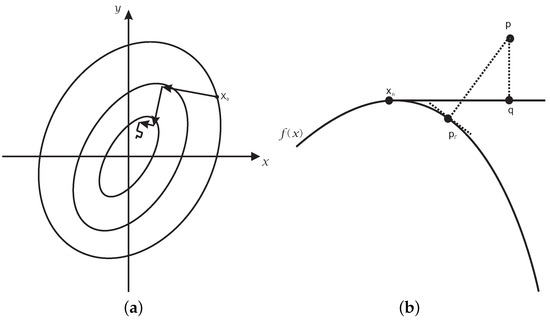
where ${\displaystyle {\mathrm{t}}_0=\frac{\left[-f_y,f_x\right]}{∥\nabla f∥}}$, $\Delta \mathrm{s}=∥\mathrm{q}-{\mathrm{x}}_n∥$. q is the corresponding orthogonal projection point of test point p at the tangent line determined by the initial iterative point ${\mathrm{x}}_n$ (see Figure 1). Formula (14) can be expressed as,

$$\left\{\begin{array}{c}\mathrm{q}=\mathrm{p}-(⟨(\mathrm{p}-{\mathrm{x}}_n),\nabla f{(\mathrm{x}}_n)⟩/⟨\nabla f{(\mathrm{x}}_n),\nabla f{(\mathrm{x}}_n)⟩)\nabla f{(\mathrm{x}}_n),\hfill \\ {\mathrm{x}}_{n+1}{=\mathrm{y}}_n{=\mathrm{x}}_n+sign\left(⟨\mathrm{p}-{\mathrm{x}}_n,{\mathrm{t}}_0⟩\right){\mathrm{t}}_0\Delta \mathrm{s}.\hfill \end{array}\right.$$

(15)

where ${\mathrm{x}}_n$ is the initial iterative point. Many numerical tests illustrate that iterative Formula (15) depends on the initial iterative point, namely it is very difficult for the iterative value ${\mathrm{y}}_n$ to fall on the planar implicit curve.

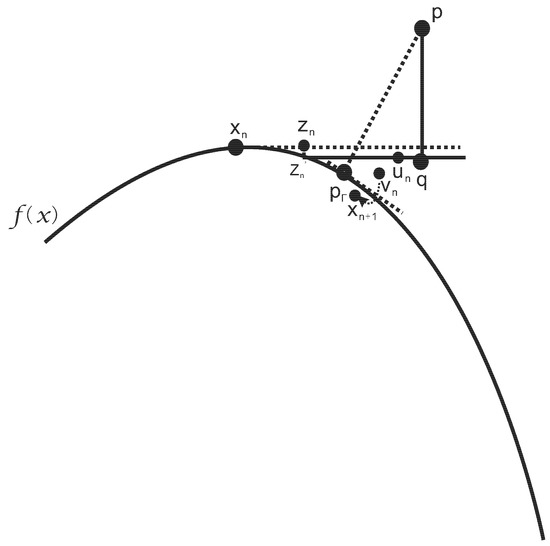
Figure 1. Graphic demonstration for the hybrid second order algorithm.

3.2. Steepest Descent Method

To move the iterative value ${\mathrm{y}}_n$ to fall on the planar implicit curve $f\left(\mathrm{x}\right)$ as much as possible, a method of preprocessing is introduced. Before the implementation of the iterative Formula (15), the steepest descent method will be adopted, namely a basic Newton’s iterative formula is added such that the iterative value ${\mathrm{y}}_n$ falls on the planar implicit curve $f\left(\mathrm{x}\right)$ as much as possible.

$$\left\{\begin{array}{c}{\mathrm{y}}_n={\mathrm{x}}_n-\left(f\left({\mathrm{x}}_n\right)/⟨\nabla f\left({\mathrm{x}}_n\right),\nabla f\left({\mathrm{x}}_n\right)⟩\right)\nabla f\left({\mathrm{x}}_n\right),\hfill \\ \mathrm{q}=\mathrm{p}-(⟨(\mathrm{p}-{\mathrm{y}}_n),\nabla f{(\mathrm{y}}_n)⟩/⟨\nabla f{(\mathrm{y}}_n),\nabla f{(\mathrm{y}}_n)⟩)\nabla f{(\mathrm{y}}_n),\hfill \\ {\mathrm{x}}_{n+1}={\mathrm{z}}_n={\mathrm{y}}_n+sign\left(⟨\mathrm{p}-{\mathrm{y}}_n,{\mathrm{t}}_0⟩\right){\mathrm{t}}_0\Delta s,\hfill \end{array}\right.$$

(16)

where ${\displaystyle {\mathrm{t}}_0=\frac{\left[-f_y,f_x\right]}{∥\nabla f∥}}$, $\Delta s=∥\mathrm{q}-{\mathrm{y}}_n∥$.

3.3. Linear Calibrating Method

Although more robust than the iterative Formula (15) to a certain extent, the iterative Formula (16) will often change convergence if the test point p or the initial iterative point ${\mathrm{x}}_0$ takes different values. Especially for large $\Delta s$, iterative point ${\mathrm{z}}_n$ will deviate from the planar implicit curve greatly, namely $\left|f\left({\mathrm{z}}_n\right)\right|=\left|\Delta e\right|>\epsilon$. In this case, a correction for the deviation of iterative point ${\mathrm{z}}_n$ is proposed as follows. If $\left|f\left({\mathrm{z}}_n\right)\right|>\epsilon$, the increment $\delta {\mathrm{z}}_n=\left[\delta x,\delta y\right]$ is used for correction. That is to say, ${\mathrm{z}}_n^{\prime }={\mathrm{z}}_n+\delta {\mathrm{z}}_n$, ${\mathrm{z}}_n$ and ${\mathrm{z}}_n^{\prime }$ are the iteration values before and after correction, respectively, and $\left|f\left({\mathrm{z}}_n^{\prime }\right)\right|<\epsilon$. The correction aims to make the deviation of the iteration value ${\mathrm{z}}_n^{\prime }$ from the planar implicit curve as small as possible. Let $\delta {\mathrm{z}}_n$ be perpendicular to increment value $\Delta {\mathrm{z}}_n=sign(\Delta s){\mathrm{t}}_0\Delta s$ and orthogonal to the planar implicit curve such that $⟨\delta {\mathrm{z}}_n,\Delta {\mathrm{z}}_n⟩=0$ and $⟨\nabla f,\delta {\mathrm{z}}_n⟩=-\Delta e$, where $\nabla f$ and $\Delta e$ take the value at ${\mathrm{z}}_n$. Then, it is easy to get $\delta {\mathrm{z}}_n=\left[-\Delta e,0\right]{\left[\nabla f^T,{(\Delta {\mathrm{z}}_n)}^T\right]}^{-1}$ and ${\mathrm{z}}_n^{\prime }={\mathrm{z}}_n+\left[-\Delta e,0\right]{\left[\nabla f^T,(\Delta {\mathrm{z}}_n{)}^T\right]}^{-1}$. The corresponding iterative formula for correction will be,

$$\left\{\begin{array}{c}{\mathrm{y}}_n={\mathrm{x}}_n-\left(f\left({\mathrm{x}}_n\right)/⟨\nabla f\left({\mathrm{x}}_n\right),\nabla f\left({\mathrm{x}}_n\right)⟩\right)\nabla f\left({\mathrm{x}}_n\right),\hfill \\ \mathrm{q}=\mathrm{p}-(⟨(\mathrm{p}-{\mathrm{y}}_n),\nabla f{(\mathrm{y}}_n)⟩/⟨\nabla f{(\mathrm{y}}_n),\nabla f{(\mathrm{y}}_n)⟩)\nabla f{(\mathrm{y}}_n),\hfill \\ {\mathrm{z}}_n={\mathrm{y}}_n+sign\left(⟨\mathrm{p}-{\mathrm{y}}_n,{\mathrm{t}}_0⟩\right){\mathrm{t}}_0\Delta s,\hfill \\ {\mathrm{x}}_{n+1}={\mathrm{z}}_n+\left[-\Delta e,0\right]{\left[\nabla f^T,(\Delta {\mathrm{z}}_n{)}^T\right]}^{-1},\hfill \end{array}\right.$$

(17)

where ${\displaystyle {\mathrm{t}}_0=\frac{\left[-f_y,f_x\right]}{∥\nabla f∥}}$, $\Delta \mathrm{s}=∥\mathrm{q}-{\mathrm{y}}_n∥$, $\Delta {\mathrm{z}}_n=sign\left(⟨\mathrm{p}-{\mathrm{z}}_n,{\mathrm{t}}_0⟩\right){\mathrm{t}}_0\Delta s$, $f\left({\mathrm{z}}_n\right)=\Delta e$. Obviously the stability and efficiency of the iterative Formula (17) improve greatly, compared with the previous iterative Formulas (15) and (16).

3.4. Newton’s Accelerated Method

Many tests for the iterative Formula (17) conducted indicate that it is sometimes not convergent when the test point lies far from the planar implicit curve. Newton’s accelerated method is then adopted to correct the problem. For the classic Newton second order iterative method, its iterative expression is:

$${\mathrm{x}}_{n+1}={\mathrm{x}}_n-\left({\mathrm{F}}_0\left({\mathrm{x}}_n\right)/⟨\nabla {\mathrm{F}}_0\left({\mathrm{x}}_n\right),\nabla {\mathrm{F}}_0\left({\mathrm{x}}_n\right)⟩\right)\nabla {\mathrm{F}}_0\left({\mathrm{x}}_n\right),$$

(18)

where $⟨\nabla {\mathrm{F}}_0\left(\mathrm{x}\right),\nabla {\mathrm{F}}_0\left(\mathrm{x}\right)⟩$ is inner product of the gradient of the function ${\mathrm{F}}_0\left(\mathrm{x}\right)$ with itself. The function ${\mathrm{F}}_0\left(\mathrm{x}\right)$ is expressed as,

$${\mathrm{F}}_0\left(\mathrm{x}\right)=\left[\left(\mathrm{p}-\mathrm{x}\right)\times \nabla f\left(\mathrm{x}\right)\right]=0,$$

(19)

where the symbol [ ] denotes the determinant of a matrix $(\mathrm{p}-\mathrm{x})\times \nabla f\left(\mathrm{x}\right)$. In order to improve the stability and rate of convergence, based on the iterative Formula (17), the hybrid second order algorithm is proposed to orthogonally project onto the planar implicit curve $f\left(\mathrm{x}\right)$. Between Step 1 and Step 2 of the iterative Formula (17) and between Step 3 and Step 4 of the same formula, the iterative Formula (18) is inserted twice. After this, the stability, the rapidity, the efficiency and the numerical iterative accuracy of the iterative algorithm (17) all improve. Then, the iterative formula becomes,

$$\left\{\begin{array}{c}{\mathrm{y}}_n={\mathrm{x}}_n-\left(f\left({\mathrm{x}}_n\right)/⟨\nabla f\left({\mathrm{x}}_n\right),\nabla f\left({\mathrm{x}}_n\right)⟩\right)\nabla f\left({\mathrm{x}}_n\right),\hfill \\ {\mathrm{z}}_n={\mathrm{y}}_n-\left({\mathrm{F}}_0\left({\mathrm{y}}_n\right)/⟨\nabla {\mathrm{F}}_0\left({\mathrm{y}}_n\right),\nabla {\mathrm{F}}_0\left({\mathrm{y}}_n\right)⟩\right)\nabla {\mathrm{F}}_0\left({\mathrm{y}}_n\right),\hfill \\ \mathrm{q}=\mathrm{p}-(⟨(\mathrm{p}-{\mathrm{z}}_n),\nabla f{(\mathrm{z}}_n)⟩/⟨\nabla f{(\mathrm{z}}_n),\nabla f{(\mathrm{z}}_n)⟩)\nabla f{(\mathrm{z}}_n),\hfill \\ {\mathrm{u}}_n={\mathrm{z}}_n+sign\left(⟨\mathrm{p}-{\mathrm{z}}_n,{\mathrm{t}}_0⟩\right){\mathrm{t}}_0\Delta s,\hfill \\ {\mathrm{v}}_n={\mathrm{u}}_n-\left({\mathrm{F}}_0\left({\mathrm{u}}_n\right)/⟨\nabla {\mathrm{F}}_0\left({\mathrm{u}}_n\right),\nabla {\mathrm{F}}_0\left({\mathrm{u}}_n\right)⟩\right)\nabla {\mathrm{F}}_0\left({\mathrm{u}}_n\right),\hfill \\ {\mathrm{x}}_{n+1}{=\mathrm{v}}_n+\left[-\Delta e,0\right]{\left[\nabla f^T,(\Delta {\mathrm{v}}_n{)}^T\right]}^{-1}(if\left|\left[\nabla f^T,(\Delta {\mathrm{v}}_n{)}^T\right]\right|=0,{\mathrm{x}}_{n+1}{=\mathrm{v}}_n).\hfill \end{array}\right.$$

(20)

where ${\displaystyle {\mathrm{t}}_0=\frac{\left[-f_y,f_x\right]}{∥\nabla f∥}}$, $\Delta \mathrm{s}=∥\mathrm{q}-{\mathrm{z}}_n∥$, $f\left({\mathrm{v}}_n\right)=\Delta e$, $\Delta {\mathrm{v}}_n=-\left({\mathrm{F}}_0\left({\mathrm{u}}_n\right)/⟨\nabla {\mathrm{F}}_0\left({\mathrm{u}}_n\right),\nabla {\mathrm{F}}_0\left({\mathrm{u}}_n\right)⟩\right)\nabla {\mathrm{F}}_0\left({\mathrm{u}}_n\right)$. Iterative termination for the iterative Formula (20) satisfies: $∥{\mathrm{x}}_{n+1}-{\mathrm{x}}_n∥<\epsilon$. The robustness and the stability of the iterative Formula (20) improves, compared with the previous iteration formulas. That is to say, even for test point p being far away from the planar implicit curve, the iterative Formula (20) is still convergent.

After normalization of the second equation and the fifth equation in the iterative Formula (20), it becomes,

$$\left\{\begin{array}{c}{\mathrm{y}}_n={\mathrm{x}}_n-\left(f\left({\mathrm{x}}_n\right)/⟨\nabla f\left({\mathrm{x}}_n\right),\nabla f\left({\mathrm{x}}_n\right)⟩\right)\nabla f\left({\mathrm{x}}_n\right),\hfill \\ {\mathrm{z}}_n={\mathrm{y}}_n-\left(\mathrm{F}\left({\mathrm{y}}_n\right)/⟨\nabla \mathrm{F}\left({\mathrm{y}}_n\right),\nabla \mathrm{F}\left({\mathrm{y}}_n\right)⟩\right)\nabla \mathrm{F}\left({\mathrm{y}}_n\right),\hfill \\ \mathrm{q}=\mathrm{p}-(⟨(\mathrm{p}-{\mathrm{z}}_n),\nabla f{(\mathrm{z}}_n)⟩/⟨\nabla f{(\mathrm{z}}_n),\nabla f{(\mathrm{z}}_n)⟩)\nabla f{(\mathrm{z}}_n),\hfill \\ {\mathrm{u}}_n={\mathrm{z}}_n+sign\left(⟨\mathrm{p}-{\mathrm{z}}_n,{\mathrm{t}}_0⟩\right){\mathrm{t}}_0\Delta s,\hfill \\ {\mathrm{v}}_n={\mathrm{u}}_n-\left(\mathrm{F}\left({\mathrm{u}}_n\right)/⟨\nabla \mathrm{F}\left({\mathrm{u}}_n\right),\nabla \mathrm{F}\left({\mathrm{u}}_n\right)⟩\right)\nabla \mathrm{F}\left({\mathrm{u}}_n\right),\hfill \\ {\mathrm{x}}_{n+1}{=\mathrm{v}}_n+\left[-\Delta e,0\right]{\left[\nabla f^T,(\Delta {\mathrm{v}}_n{)}^T\right]}^{-1}(if\left|\left[\nabla f^T,{(\Delta {\mathrm{v}}_n)}^T\right]\right|=0,{\mathrm{x}}_{n+1}={\mathrm{v}}_n),\hfill \end{array}\right.$$

(21)

where $\mathrm{F}\left(\mathrm{x}\right)=\frac{{\mathrm{F}}_0\left(\mathrm{x}\right)}{{\displaystyle \sqrt{⟨\nabla f\left(\mathrm{x}\right),\nabla f\left(\mathrm{x}\right)⟩}}}$. The iterative Formula (21) can be implemented in six steps. The first step computes the point ${\mathrm{x}}_n$ on the planar implicit curve using the basic Newton’s iterative formula, which is not associated with test point p for any initial iterative point. The second step uses Newton’s iterative method to accelerate the whole iteration process and get the new iterative point ${\mathrm{z}}_n$, which is associated with test point p. The third step gets the orthogonal projection point q (footpoint) at the tangent line to $f\left(\mathrm{x}\right)$. The fourth equation in iterative Formula (21) yields the new iterative point ${\mathrm{u}}_n$. The third step and the fourth step compute the linear orthogonal increment, which is the core component (including linear calibrating method of sixth step) of the iterative Formula (21). The fifth step accelerates the previous steps again and yields the iterative point, which is associated with test point p. The sixth step corrects the iterative result for the previous three steps. Therefore, the whole six steps ensure the robustness of the whole iteration process. The above procedure is repeated until the iterative point coincides with the orthogonal projection point ${\mathrm{p}}_{\Gamma }$ (see Figure 1 and the detailed explanation of Remark 3).

Remark 1.

In the actual implementation of the iterative Formula (21) of the hybrid second order algorithm (Algorithm 1), three techniques are used to optimize the process. On the right-hand side of Step 1, Step 2, Step 3 and step 5, the part in parentheses is calculated firstly and then the part outside the parentheses to prevent overflow of the intermediate calculation process. Error handling for the second term is added in the right-hand side of Step 4 in the iterative Formula (21). Namely, if $⟨p-z_n,t_0⟩=0$, sign $\left(⟨p-z_n,t_0⟩\right)$ = 1. For the second term of the right-hand side in Step 6 of the iterative Formula (21), if the determinant of $\left[\nabla f^T,{(\Delta v_n)}^T\right]$ is zero, then $x_{n+1}=v_n$. Namely, if any component of $\left[-\Delta e,0\right]{\left[\nabla f^T,{(\Delta v_n)}^T\right]}^{-1}$ equals zero, then substitute the sixth step with $x_{n+1}=v_n$ to avoid the overflow problem.

According to the analyses above, the hybrid second order algorithm is presented as follows.

Algorithm 1: Hybrid second order algorithm.

Input: Initial iterative value ${\mathrm{x}}_0$, test point p and planar implicit curve $f\left(\mathrm{x}\right)=0$.

Output: The orthogonal projection point ${\mathrm{p}}_{\Gamma }$.

Description:

Step 1:

${\mathrm{x}}_{n+1}={\mathrm{x}}_0$;

do{

${\mathrm{x}}_n={\mathrm{x}}_{n+1}$;

Update ${\mathrm{x}}_{n+1}$ according to the iterative Formula (21);

}while(${∥{\mathrm{x}}_{n+1}-{\mathrm{x}}_n∥}^2>{\epsilon }_1$);

Step 2:

${\mathrm{p}}_{\Gamma }$ = ${\mathrm{x}}_{n+1}$;

return ${\mathrm{p}}_{\Gamma }$;

Remark 2.

Many tests demonstrate that if the test point p is not far away from the planar implicit curve, Algorithm 1 will converge for any initial iterative point $x_0$. For instance, assume a planar implicit curve $f(x,y)=x^6+2x^{5}y-2x^3{y}^2+x^4-y^3+2y^8-4$ and four different test points $(13,7),(3,-4),(-2,2),(-7,-3)$; Algorithm 1 converges efficiently for the given initial iterative value. See Table 1 for details, where p is the test point, $x_0$ is the initial iterative point, iterations is the number of iterations, $\left|f\left(p_{\Gamma }\right)\right|$ is the absolute function value with the orthogonal projection point $p_{\Gamma }$ and Error_2 = $\left|\left[(p-p_{\Gamma })\times \nabla f\left(p_{\Gamma }\right)\right]\right|$.

Table 1. Convergence of the hybrid second order algorithm for four given test points.

p	(13,7)	(3,−4)	(−2,2)	(−7,−3)
${\mathrm{x}}_0$	(2,2)	(3,−2)	(−1.5,1.5)	(−1,−1)
Iterations	35	49	11	48
${\mathrm{p}}_{\Gamma }$	(1.0677273301335340, 0.98814885115384405)	(3.2064150662530660, −1.8804902065934096)	(−1.1847729458379061, 0.97069828125793904)	(−0.96286546696734312, −0.67794903011569976)
$\left|f\left({\mathrm{p}}_{\Gamma }\right)\right|$	0	$3.5218\times {10}^{-10}$	$9.153595\times {10}^{-10}$	$1.0\times {10}^{-16}$
Error_2	$2.7\times {10}^{-13}$	$6.1\times {10}^{-14}$	$8.0\times {10}^{-16}$	$3.5389\times {10}^{-11}$

However, when the test point p is far away from the planar implicit curve, no matter whether the initial iterative point p is close to the planar implicit curve, Algorithm 1 sometimes produces oscillation such that subsequent iterations could not ensure convergence. For example, for the same planar implicit curve with test point p = $(17,-11)$ and initial iterative point ${\mathrm{x}}_0$ = $(2,-2)$, it constantly produces oscillation such that subsequent iterations could not ensure convergence after 838 iterations (see Table 2).

Table 2. Oscillation of the hybrid second order algorithm for the planar implicit curve with a far-away test point.

Iterations	691	703	709	715	721
${\mathrm{x}}_n$	(16.5606,−6.3965)	(16.8426,−7.0908)	(8.7616,−3.3728)	(16.9335,−7.5757)	(9.3579,−3.5205)
$\left|f\left(x_n\right)\right|$	10,001,975.0670	15,989,718.8891	128,212.4352	23,705,389.2353	200,851.6993
Iterations	727	733	739	745	751
${\mathrm{x}}_n$	(16.9837,−8.1857)	(10.1857,−3.7217)	(16.9979,−8.6470)	(10.7849,−3.8660)	(3.4438,−3.2804)
$\left|f\left(x_n\right)\right|$	40,608,498.6528	355,827.4721	61,442,889.2860	521,346.2808	24,602.7729
Iterations	761	771	781	791	801
${\mathrm{x}}_n$	(6.9925,−2.9214)	(9.5387,−3.5647)	(12.0328,−4.1693)	(15.6601,−5.4760)	(16.9137,−7.4381)
$\left|f\left(x_n\right)\right|$	26,408.0394	228,676.1751	1,074,966.2463	5,881,539.2784	21,106,110.9316
Iterations	811	821	831	832	833
${\mathrm{x}}_n$	(4.6652,−2.1979)	(8.1550,−3.2191)	(10.9409,−3.9036)	(9.4499,−3.5430)	(8.3148,−3.2592)
$\left|f\left(x_n\right)\right|$	1183.7775	78,196.8686	573,585.9893	214,640.2588	89,454.0288
Iterations	834	835	836	837	838
${\mathrm{x}}_n$	(7.5358,−3.0631)	(5.9435,−2.6227)	(4.3903,−1.8397)	(5.3516,−6.3813)	(17.0038,−9.5117)
$\left|f\left(x_n\right)\right|$	44,975.5254	8028.5679	1222.8394	5,455,596.6976	130,321,659.7406

3.5. Initial Iterative Value Estimation Algorithm

Through Remark 2, when the test point p is not far away from the planar implicit curve, with the initial iterative point ${\mathrm{x}}_0$ in any position, Algorithm 1 could ensure convergence. However, when the test point p is far away from the planar implicit curve, even if the initial iterative point ${\mathrm{x}}_0$ is close to the planar implicit curve, Algorithm 1 sometimes produces oscillation such that subsequent iterations could not ensure convergence. This is essentially a problem for any Newton-based method. Consider high nonlinearity, which cannot be captured just by $f(x,y)=0$, i.e, the surface $[x,y,f(x,y\left)\right]$ is very oscillatory in the neighborhood of the $\mathrm{z}=0$ plane, but it does intersect the $\mathrm{z}=0$ plane in a single closed branch. Under this case, for far-away test point p from the planar implicit curve, any Newton-based method sometimes will produce oscillation to cause non-convergence. We will give a counter example in Remark 2. To solve the problem of non-convergence, some method is proposed to put the initial iterative point ${\mathrm{x}}_0$ close to the orthogonal projection point ${\mathrm{p}}_{\Gamma }$. Therefore, the task changes to construct an algorithm such that the initial iterative value ${\mathrm{x}}_0$ of the iterative Formula (21) and the orthogonal projection point ${\mathrm{p}}_{\Gamma }$ are as close as possible. The algorithm can be summarized as follows. Input an initial iterative point ${\mathrm{x}}_0$, and repeatedly iterate with the basic Newton’s iterative formula $\mathrm{y}=\mathrm{x}-\left(f\left(\mathrm{x}\right)/⟨\nabla f\left(\mathrm{x}\right),\nabla f\left(\mathrm{x}\right)⟩\right)\nabla f\left(\mathrm{x}\right)$ such that the iterative point lies on the planar implicit curve $f\left(\mathrm{x}\right)$ (see Figure 2c). After that, iterate once through the formula $\mathrm{q}=\mathrm{p}-(⟨(\mathrm{p}-\mathrm{x}),\nabla f\left(\mathrm{x}\right)⟩/⟨\nabla f\left(\mathrm{x}\right),\nabla f\left(\mathrm{x}\right)⟩)\nabla f\left(\mathrm{x}\right)$ where the blue point denotes the initial iterative value (see Figure 2c). After the first round iteration in Figure 2, then replace the initial iterative value with the iterated value q, and do the second round iteration (see Figure 3). After the second round iteration, replace the initial iterative value with the iterated value q, and do the third round iteration (see Figure 4). The detailed algorithm is the following.

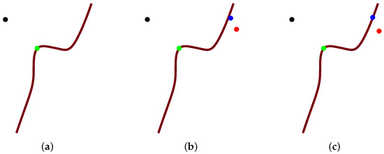
Figure 2. The entire graphical demonstration of the first round iteration in Algorithm 2. (a) Initial status; (b) Intermediate status; (c) Final status.

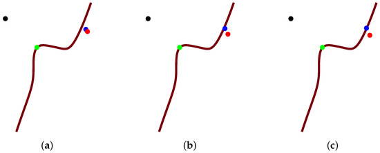
Figure 3. The entire graphical demonstration of the second round iteration in Algorithm 2. (a) Initial status; (b) Intermediate status; (c) Final status.

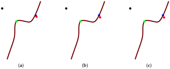
Figure 4. The entire graphical demonstration of the third round iteration in Algorithm 2. (a) Initial status; (b) Intermediate status; (c) Final status.

Firstly, the notations for Figure 2, Figure 3 and Figure 4 are clarified. Black and green points represent test point p and orthogonal projection point ${\mathrm{p}}_{\Gamma }$, respectively. The blue point denotes ${\mathrm{x}}_{n+1}={\mathrm{x}}_n-(f\left({\mathrm{x}}_n\right)/⟨\nabla f\left({\mathrm{x}}_n\right),\nabla f\left({\mathrm{x}}_n\right)⟩)\nabla f\left({\mathrm{x}}_n\right)$ of Step 2 in Algorithm 2, whether it is on the planar implicit curve $f\left(\mathrm{x}\right)$ or not. The footpoint q(red point) denotes q in Step 3 of Algorithm 2, and the brown curve describes the planar implicit curve $f\left(\mathrm{x}\right)=0$.

Secondly, Algorithm 2 is interpreted geometrically. Step 2 in Algorithm 2 uses basic Newton’s iterative method. That is to say, it repeatedly iterates using the steepest descent method in Section 3.2 until the blue point ${\mathrm{x}}_{n+1}={\mathrm{x}}_n-(f\left({\mathrm{x}}_n\right)/⟨\nabla f\left({\mathrm{x}}_n\right),\nabla f\left({\mathrm{x}}_n\right)⟩)\nabla f\left({\mathrm{x}}_n\right)$ of Step 2 lies on the planar implicit curve $f\left(\mathrm{x}\right)$. At the same time, through Step 3 in Algorithm 2, it yields footpoint q (see Figure 2). The integer n of the iteration round counts one after the first round iteration of Algorithm 2. When the blue point is on the planar implicit curve $f\left(\mathrm{x}\right)$, at this time, replace the initial iterative value with the iterated value q, and do the second round iteration; the integer n of the iteration round counts two (see Figure 3). Replace the initial iterative value with the iterated value q again after the second round iteration, and do the third round iteration; the integer n of the iteration round counts three (see Figure 4). When $n=3$ in Step 4, then exit Algorithm 2. At this time, the current footpoint q from Algorithm 2 will be the initial iterative value for Algorithm 1.

Algorithm 2: Initial iterative value estimation algorithm.

Input: Initial iterative value ${\mathrm{x}}_0$, test point p and planar implicit curve $f\left(\mathrm{x}\right)=0$.

Output: The footpoint point q.

Description:

Step 1: $n=0$; ${\mathrm{x}}_{n+1}={\mathrm{x}}_0$;

Step 2:

do{

${\mathrm{x}}_n={\mathrm{x}}_{n+1}$;

${\mathrm{x}}_{n+1}={\mathrm{x}}_n-\left(f\left({\mathrm{x}}_n\right)/⟨\nabla f\left({\mathrm{x}}_n\right),\nabla f\left({\mathrm{x}}_n\right)⟩\right)\nabla f\left({\mathrm{x}}_n\right)$;

}while(${∥{\mathrm{x}}_{n+1}-{\mathrm{x}}_n∥}^2>{\epsilon }_2$);

Step 3: $\mathrm{q}=\mathrm{p}-(⟨(\mathrm{p}-{\mathrm{x}}_{n+1}),\nabla f{(\mathrm{x}}_{n+1})⟩/⟨\nabla f{(\mathrm{x}}_{n+1}),\nabla f{(\mathrm{x}}_{n+1})⟩)\nabla f{(\mathrm{x}}_{n+1})$;

Step 4: $n=n+1$;

if $(n\le 3)$ {

${\mathrm{x}}_{n+1}=\mathrm{q}$;

go to Step 1;

}

else

return q;

Thirdly, the reason for choosing $n=3$ in Algorithm 2 is explained. Many cases are tested for planar implicit curves with no singular point. As long as $n=2$, the output value from Algorithm 2 could be used as the initial iterative value of Algorithm 1 to get convergence. However, if the planar implicit curve has singular points or big fluctuation and oscillation appear, $n=3$ can guarantee the convergence. In a future study, a more optimized and efficient algorithm needs to be developed to automatically specify the integer n.

3.6. Integrated Hybrid Second Order Algorithm

Algorithm 2 can optimize the initial iterative value for Algorithm 1. Then, Algorithm 1 can project the test point p onto planar implicit curve $f\left(\mathrm{x}\right)$. The integrated hybrid second order algorithm (Algorithm 3) is presented to take advantage of Algorithms 1 and 2, which are denoted as Algorithm 1 (${(\mathrm{x}}_0,\mathrm{p},f\left(\mathrm{x}\right))$ and Algorithm 2 ($\mathrm{q},\mathrm{p},f\left(\mathrm{x}\right))$ for convenience, respectively. Algorithm 3 can be described as follows (see Figure 5).

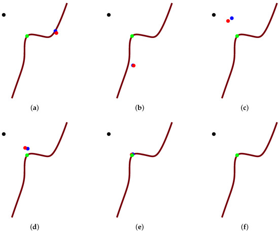
Figure 5. The entire graphical demonstration for the whole iterative process of Algorithm 3. (a) Initial status; (b) First intermediate status; (c) Second intermediate status; (d) Third intermediate status; (e) Fourth intermediate status; (f) Final status.

Firstly, the notations for Figure 5 are clarified, which describes the entire iterative process in Algorithm 3. The black point is test point p; the green point is orthogonal projection point ${\mathrm{p}}_{\Gamma }$; the blue point is the left-hand side value of the equality of the first step of the iterative Formula (21) in Algorithm 1; footpoint q (red point) is the left-hand side value of the equality of the third step of the iterative Formula (21) in Algorithm 1; and the brown curve represents the planar implicit curve $f\left(\mathrm{x}\right)$.

Algorithm 3: Integrated hybrid second order algorithm.

Input: Initial iterative value ${\mathrm{x}}_0$, test point p and planar implicit curve $f\left(\mathrm{x}\right)=0$.

Output: The orthogonal projection point ${\mathrm{p}}_{\Gamma }$.

Description:

Step 1: q = Algorithm 2 ${(\mathrm{x}}_0,\mathrm{p},f\left(\mathrm{x}\right))$;

Step 2: ${\mathrm{p}}_{\Gamma }$ = Algorithm 1 $(\mathrm{q},\mathrm{p},f\left(\mathrm{x}\right))$;

Step 3: return ${\mathrm{p}}_{\Gamma }$;

Secondly, Algorithm 3 is interpreted. The output from Algorithm 2 is taken as the initial iterative value for Algorithm 1 (see footpoint q or the red point in Figure 4c). Algorithm 1 repeatedly iterates until it satisfies the termination criteria ($∥{\mathrm{x}}_{n+1}-{\mathrm{x}}_n∥<\epsilon )$ (see Figure 5). The six subgraphs in Figure 5 represent successive steps in the entire iterative process of Algorithm 1. In the end, three points of green, blue and red merge into orthogonal projection point ${\mathrm{p}}_{\Gamma }$ (see Figure 5f).

Remark 3.

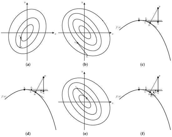
Algorithm 3 with two sub-algorithms is interpreted geometrically, where Algorithms 1 and 2 are graphically demonstrated by Figure 6 and Figure 7, respectively. In Figure 6a and Figure 7a, several closed loops represent the orthogonal projection of the contour lines on the surface $z=f(x,y)$ onto the horizontal plane $x-y$, respectively. In Figure 7b,e, several closed loops also represent orthogonal projection of the contour lines on the surface $z=F(x,y)$ onto the horizontal plane $x-y$, respectively. In Figure 6a, the vector starting with point $x_0$ is gradient $-\nabla f\left(x_0\right)$, and the length of the vector is $f\left(x_0\right)/⟨\nabla f\left(x_0\right),\nabla f\left(x_0\right)⟩$. For arbitrary initial iterative point $x_0$, the iterative formula $x_{n+1}=x_n-\left(f\left(x_n\right)/⟨\nabla f\left(x_n\right),\nabla f\left(x_n\right)⟩\right)\nabla f\left(x_n\right)$ (Step 2 of Algorithm 2) from the steepest descent method repeatedly iterates until the iterative point $x_n$ lies on the planar implicit curve $f\left(x\right)$. In Figure 6b, the footpoint q, i.e., the intersection of tangent line (from the point $x_n$ on the planar implicit curve $f\left(x\right)$) and perpendicular line (from test point p) is acquired by Step 3 in Algorithm 2. After the first round iteration of Algorithm 2, replace the initial iterative point $x_0$ with the footpoint q, and then, do the second round and the third round iteration. The three rounds of iteration constitute Algorithm 2 and part of Algorithm 3.

Figure 6. The entire graphical demonstration of Algorithm 2. (a) Step 2 of Algorithm 2; (b) Step 3 of Algorithm 2.

Figure 7. The entire graphical demonstration of Algorithm 1. (a) The first step of the iterative Formula (21); (b) The second step of the iterative Formula (21); (c) The third step of the iterative Formula (21); (d) The fourth step of the iterative Formula (21); (e) The fifth step of the iterative Formula (21); (f) The sixth step of the iterative Formula (21).

In each sub-figure of Figure 7, points p and ${\mathrm{p}}_{\Gamma }$ are the test point and the corresponding orthogonal projective point, respectively. In Figure 7a, the vector starting with point ${\mathrm{x}}_n$ is gradient $-\nabla f\left({\mathrm{x}}_n\right)$, and the length of the vector is $f\left({\mathrm{x}}_n\right)/⟨\nabla f\left({\mathrm{x}}_n\right),\nabla f\left({\mathrm{x}}_n\right)⟩$. For the initial iterative point ${\mathrm{x}}_n$ from Algorithm 2, the iterative formula ${\mathrm{y}}_n={\mathrm{x}}_n-\left(f\left({\mathrm{x}}_n\right)/⟨\nabla f\left({\mathrm{x}}_n\right),\nabla f\left({\mathrm{x}}_n\right)⟩\right)\nabla f\left({\mathrm{x}}_n\right)$ (Step 1 of Algorithm 1) from the steepest descent method iterates once. In Figure 7b, the vector starting with point ${\mathrm{y}}_n$ is gradient $-\nabla \mathrm{F}\left({\mathrm{y}}_n\right)$, and the length of the vector is $\mathrm{F}\left({\mathrm{y}}_n\right)/⟨\nabla \mathrm{F}\left({\mathrm{y}}_n\right),\nabla \mathrm{F}\left({\mathrm{y}}_n\right)⟩$. For the initial iterative point ${\mathrm{y}}_n$ from Step 1 in Algorithm 1, $\mathrm{F}\left(\mathrm{x}\right)=\frac{\left[(\mathrm{p}-\mathrm{x})\times \nabla f\left(\mathrm{x}\right)\right]}{\sqrt{⟨\nabla f\left(\mathrm{x}\right),\nabla f\left(\mathrm{x}\right)⟩}}$, the iterative formula ${\mathrm{z}}_n={\mathrm{y}}_n-\left(\mathrm{F}\left({\mathrm{y}}_n\right)/⟨\nabla \mathrm{F}\left({\mathrm{y}}_n\right),\nabla \mathrm{F}\left({\mathrm{y}}_n\right)⟩\right)\nabla \mathrm{F}\left({\mathrm{y}}_n\right)$ (Step 2 of Algorithm 1) from the steepest descent method iterates once. In Figure 7c, the footpoint q, i.e., the intersection of tangent line (from the point ${{\mathrm{z}}^{\prime }}_n$ on the planar implicit curve $f\left(\mathrm{x}\right)$) and the perpendicular line (from test point p), is acquired by Step 3 in Algorithm 1. In the actual iterative process, point ${{\mathrm{z}}^{\prime }}_n$ is approximately equivalent to the point ${\mathrm{z}}_n$. In Figure 7d, point ${\mathrm{u}}_n$ comes form the fourth step of Algorithm 1, which aims to obtain a linear orthogonal increment. In Figure 7e, the vector starting with point ${\mathrm{u}}_n$ is gradient $-\nabla \mathrm{F}\left({\mathrm{u}}_n\right)$, and the length of the vector is $F\left({\mathrm{u}}_n\right)/⟨\nabla \mathrm{F}\left({\mathrm{u}}_n\right),\nabla \mathrm{F}\left({\mathrm{u}}_n\right)⟩$. For the initial iterative point ${\mathrm{u}}_n$ from Step 4 in Algorithm 1, the iterative formula ${\mathrm{v}}_n={\mathrm{u}}_n-\left(\mathrm{F}\left({\mathrm{u}}_n\right)/⟨\nabla \mathrm{F}\left({\mathrm{u}}_n\right),\nabla \mathrm{F}\left({\mathrm{u}}_n\right)⟩\right)\nabla \mathrm{F}\left({\mathrm{u}}_n\right)$ (Step 5 of Algorithm 1) from the steepest descent method iterates once more. In Figure 7f, the iterative point ${\mathrm{x}}_{n+1}$ from the sixth step in Algorithm 1 gives a correction for the iterative point ${\mathrm{v}}_n$ from the fifth step in Algorithm 1. Repeatedly iterate the above six steps until the iteration exit criteria are met. In the end, three points of footpoint q, the iterative point ${\mathrm{x}}_{n+1}$ and the orthogonal projecting point ${\mathrm{p}}_{\Gamma }$ merge into orthogonal projection point ${\mathrm{p}}_{\Gamma }$. These six steps constitute Algorithm 1 and part of Algorithm 3.

4. Convergence Analysis

In this section, the convergence analysis for the integrated hybrid second order algorithm is presented. Proofs indicate the convergence order of the algorithm is up to two, and Algorithm 3 is independent of the initial value.

Theorem 1.

Given an implicit function $f\left(x\right)$ that can be parameterized, the convergence order of the iterative Formula (21) is up to two.

Proof. 

Without loss of generality, assume that the parametric representation of the planar implicit curve $\Gamma :f(\mathrm{x})=0$ is $c\left(t\right)=(f_1\left(t\right),f_2\left(t\right))$. Suppose that parameter $\alpha$ is the orthogonal projection point of test point $\mathrm{p}=(p_1,p_2)$ onto the parametric curve $c\left(t\right)=(f_1\left(t\right),f_2\left(t\right))$. ☐

The first part will derive that the order of convergence of the first step for the iterative Formula (21) is up to two. It is not difficult to know the iteration equation in the corresponding Newton’s second order parameterized iterative method, i.e., the first step for the iterative Formula (21):

$$t_{n+1}=t_n-\frac{c\left(t_n\right)}{c^{\prime }\left(t_n\right)}.$$

(22)

Taylor expansion around $\alpha$ generates:

$$c\left(t_n\right)=c_0+c_1{e}_n+c_2{e}_n^2+o\left(e_n^3\right),$$

(23)

where $e_n=t_n-\alpha$ and $c_i=(1/i!)\left(f^{\left(i\right)}\left(\alpha \right)\right),i=0,1,2$. Thus, it is easy to have:

$$c^{\prime }\left(t_n\right)=c_1+2c_2{e}_n+o\left(e_n^2\right).$$

(24)

From (22)–(24), the error iteration can be expressed as,

$$e_{n+1}=C_0{e}_n^2+o\left(e_n^3\right),$$

(25)

where ${\displaystyle C_0=\frac{c_2}{c_1}}$.

The second part will prove that the order of convergence of the second step for the iterative Formula (21) is two. It is easy to get the corresponding parameterized iterative equation for Newton’s second-order iterative method, essentially the second step for the iterative Formula (21),

$$t_{n+1}=t_n-\frac{\mathrm{F}\left(t_n\right)}{{\mathrm{F}}^{\prime }\left(t_n\right)},$$

(26)

where:

$$\mathrm{F}(t)=⟨\mathrm{p}-c\left(t\right),c^{\prime }\left(t\right)⟩=0.$$

(27)

Using Taylor expansion around $\alpha$, it is easy to get:

$$\mathrm{F}\left(t_n\right)=b_0+b_1{e}_n+b_2{e}_n^2+o\left(e_n^3\right),$$

(28)

where $e_n=t_n-\alpha$ and $b_i=(1/i!)\left({\mathrm{F}}^{\prime }\left(\alpha \right)\right),i=0,1,2$. Thus, it is easy to get:

$${\mathrm{F}}^{\prime }\left(t_n\right)=b_1+2b_2{e}_n+o\left(e_n^2\right).$$

(29)

According to Formula (26)–(29), after Taylor expansion and simplifying, the error relationship can be expressed as follows,

$$e_{n+1}=C_1{e}_n^2+o\left(e_n^3\right),$$

(30)

where ${\displaystyle C_1=\frac{b_2}{b_1}}$. Because the fifth step is completely equal to the second step of the iterative Formula (21) and outputs from Newton’s iterative method are closely related with test point p, the order of convergence for the fifth step of the iterative Formula (21) is also two.

The third part will derive that the order of convergence of the third step and fourth step for iterative Formula (21) is one. According to the first order method for orthogonal projection onto the parametric curve [32,39,40], the footpoint $\mathrm{q}=(q_1,q_2)$ of the parameterized iterative equation of the third step of the iterative Formula (21) can be expressed in the following way,

$$\mathrm{q}=c\left(t_n\right)+\Delta t{c}^{\prime }\left(t_n\right).$$

(31)

From the iterative Equation (31) and combining with the fourth step of the iterative Formula (21), it is easy to have:

$$\Delta t=\frac{⟨c^{\prime }\left(t_n\right),\mathrm{q}-c\left(t_n\right)⟩}{⟨c^{\prime }\left(t_n\right),c^{\prime }\left(t_n\right)⟩,}$$

(32)

where $⟨x,y⟩$ denotes the scalar product of vectors $x,y\in R^2$. Let $t_n+\Delta t\to t_n$, and repeat the procedure (32) until $\Delta t$ is less than a given tolerance $\epsilon$. Because parameter $\alpha$ is the orthogonal projection point of test point $\mathrm{p}=(p_1,p_2)$ onto the parametric curve $c\left(t\right)=(f_1\left(t\right),f_2\left(t\right))$, it is not difficult to verify,

$$⟨\mathrm{p}-c\left(\alpha \right),c^{\prime }\left(\alpha \right)⟩=0.$$

(33)

Because the footpoint q is the intersection of the tangent line of the parametric curve $c\left(t\right)$ at $t=t_n$ and the perpendicular line $\overrightarrow{\mathrm{p}\mathrm{q}}$ determined by the test point p, the equation of the tangent line of the parametric curve $c\left(t\right)$ at $t=t_n$ is:

$$\left\{\begin{array}{c}{x}_1=f_1\left(t_n\right)+f_1^{\prime }\left(t_n\right)s,\hfill \\ x_2=f_2\left(t_n\right)+f_2^{\prime }\left(t_n\right)s.\hfill \end{array}\right.$$

(34)

At the same time, the vector of the line segment connected by the test point p and the point $c\left(t_n\right)$ is:

$$(y_1,y_2)=(p_1-x_1,p_2-x_2).$$

(35)

The vector (35) and the tangent vector $c^{\prime }\left(t_n\right)=(f_1^{\prime }\left(t_n\right),f_2^{\prime }\left(t_n\right))$ of the tangent line (34) are mutually orthogonal, so the parameter value $s_0$ of the tangent line (34) is:

$$s_0=\frac{⟨\mathrm{p}-c\left(t_n\right),c^{\prime }\left(t_n\right)⟩}{⟨c^{\prime }\left(t_n\right),c^{\prime }\left(t_n\right)⟩}.$$

(36)

Substituting (36) into (34) and simplifying, it is not difficult to get the footpoint q = $(q_1,q_2)$,

$$\left\{\begin{array}{c}{q}_1=f_1\left(t_n\right)+f_1^{\prime }\left(t_n\right)s_0,\hfill \\ q_2=f_2\left(t_n\right)+f_2^{\prime }\left(t_n\right)s_0.\hfill \end{array}\right.$$

(37)

Substituting (37) into (32) and simplifying, it is easy to obtain,

$$\Delta t=\frac{⟨\mathrm{p}-c\left(t_n\right),c^{\prime }\left(t_n\right)⟩}{⟨c^{\prime }\left(t_n\right),c^{\prime }\left(t_n\right)⟩}.$$

(38)

From (33) and combined with (38), using Taylor expansion by the symbolic computation software Maple 18, it is easy to get:

$$\Delta t=\frac{2c_2(c_0-\mathrm{p})-c_1^2}{c_1^2}{e}_n+o\left(e_n^2\right).$$

(39)

Simplifying (30), it is easy to obtain:

$$\begin{array}{cc}\hfill e_{n+1}=& \frac{2c_2(c_0-\mathrm{p})}{c_1^2}{e}_n+o\left(e_n^2\right),\hfill \\ \hfill =& C_2{e}_n+o\left(e_n^2\right),\hfill \end{array}$$

(40)

where the symbol $C_2$ denotes the coefficient in the first order error $e_n$ of the right-hand side of Formula (40). The result shows that the third step and the fourth step of the iterative Formula (21) comprise the first order convergence. According to the iterative Formula (21) and combined with three error iteration relationships (25), (30) and (40), the convergent order of each iterative formula is not more than two. Then, the iterative error relationship of the iterative Formula (21) can be expressed as follows:

$$e_{n+1}=C_0{C}_1{C}_2{e}_n^2+o\left(e_n^3\right).$$

(41)

To sum up, the convergence order of the iterative Formula (21) is up to two.

Theorem 2.

The convergence of the hybrid second order algorithm (Algorithm 1) is a compromise method between the local and global method.

Proof. 

The third step and fourth step of the iterative Formula (21) of Algorithm 1 are equivalent to the foot point algorithm for implicit curves in [32]. The work in [14] has explained that the convergence of the foot point algorithm for the implicit curve proposed in [14] is a compromise method between the local and global method. Then, the convergence of Algorithm 1 is also a compromise method between the local and global method. Namely, if a test point is close to the foot point of the planar implicit curve, the convergence of Algorithm 1 is independent of the initial iterative value, and if not, the convergence of Algorithm 1 is dependent on the initial iterative value. The sixth step in Algorithm 1 promotes the robustness. However, the third step, the fourth step and the sixth step in Algorithm 1 still constitute a compromise method between the local and global ones. Certainly, the first step (steepest descent method) of Algorithm 1 can make the iterative point fall on the planar implicit curve and improves its robustness. The second step and the fifth step constitute the classical Newton’s iterative method to accelerate convergence and improve robustness in some way. The steepest descent method of the first step and Newton’s iterative method of the second step and the fifth step in Algorithm 1 are more robust and efficient, but they can change the fact that Algorithm 1 is the compromise method between the local and global ones. To sum up, Algorithm 1 is the compromise method between the local and global ones. ☐

Theorem 3.

The convergence of the integrated hybrid second order algorithm (Algorithm 3) is independent of the initial iterative value.

Proof. 

The integrated hybrid second order algorithm (Algorithm 3) is composed of two parts sub-algorithms (Algorithm 1 and Algorithm 2). From Theorem 2, Algorithm 1 is a compromise method between the local and global method. Of course, whether the test point p is very far away or not far away from the planar implicit curve $f\left(\mathrm{x}\right)$, if the initial iterative value lies close to the orthogonal projection point ${\mathrm{p}}_{\Gamma }$, Algorithm 1 could be convergent. In any case, Algorithm 2 can change the initial iterative value of Algorithm 1 sufficiently close to the orthogonal projection point ${\mathrm{p}}_{\Gamma }$ to ensure the convergence of Algorithm 1. In this way, Algorithm 3 can converge for any initial iterative value. Therefore, the convergence of the integrated hybrid second order algorithm (Algorithm 3) is independent of the initial value. ☐

5. Results of the Comparison

Example 1.

([14]) Assume a planar implicit curve $\Gamma :f(x,y)=(y^5+x^3-x^2+\frac{4}{27})(\frac{x}{2}+1)=0$. One thousand and six hundred test points from the square $\left[-2,2\right]\times \left[-2,2\right]$ are taken. The integrated hybrid second order algorithm (Algorithm 3) can orthogonally project all 1600 points onto planar implicit curve Γ. It satisfies the relationships $\left|f\left({\mathrm{p}}_{\Gamma }\right)\right|<{10}^{-10}$ and $\left|\left[(p-p_{\Gamma })\times \nabla f\left(p_{\Gamma }\right)\right]\right|<{10}^{-10}$.

It consists of two steps to select/sample test points:

(1) Uniformly divide planar square $\left[-2,2\right]\times \left[-2,2\right]$ of the planar implicit curve into $m^2=1600$ sub-regions $\left[a_i,a_{i+1}\right]\times \left[c_j,c_{j+1}\right],i,j=0,1,2,\dots ,m-1$, where $a=a_0=-2,a_{i+1}-a_i=\frac{b-a}{m}=1/10,b=a_m=2,c=c_0=-2,c_{j+1}-c_j=\frac{d-c}{m}=1/10,d=c_m=2.$

(2) Randomly select a test point in each sub-region and then an initial iterative value in its vicinity.

The same procedure to select/sample test points applies for other examples below.

One test point $\mathrm{p}=(-0.1,1.0)$ in the first case is specified. Using Algorithm 3, the corresponding orthogonal projection point is ${\mathrm{p}}_{\Gamma }$ = (−0.47144354751227009, 0.70879213227958752), and the initial iterative values ${\mathrm{x}}_0$ are (−0.1,0.8), (−0.1,0.9), (−0.1,1.1), (−0.1,1.2), (−0.2,0.8), (−0.2,0.9), (−0.2,1.1) and (−0.2,1.2), respectively. Each initial iterative value iterates 12 times, respectively, yielding 12 different iteration times in nanoseconds. In Table 3, the average running times of Algorithm 3 for eight different initial iterative values are 1,099,243, 582,078, 525,942, 490,537, 392,090, 364,817, 369,739 and 367,654 nanoseconds, respectively. In the end, the overall average running time is 524,013 nanoseconds, while the overall average running time of the circle shrinking algorithm in [14] is 8.9 ms under the same initial iteration condition.

Table 3. Running time for different initial iterative values by Algorithm 3 in Example 1.

${\mathrm{x}}_0$ is the initial iterative point of Algorithm 3
${\mathrm{x}}_0$	(−0.1,0.8)	(−0.1,0.9)	(−0.1,1.1)	(−0.1,1.2)	(−0.2,0.8)	(−0.2,0.9)	(−0.2,1.1)	(−0.2,1.2)
1	1,031,458	538,050	596,727	451,274	374,678	352,327	379,469	427,197
2	101,3206	713,362	729,091	325,384	369,743	382,516	335,742	437,603
3	1045,695	579,753	547,925	471,946	380,761	316,481	372,246	381,766
4	1,078,068	602,184	479,085	509,162	354,854	354,927	327,876	388,046
5	1,051,972	455,932	452,681	472,085	380,566	289,771	382,982	277,172
6	1,091,185	607,295	488,716	509,573	316,803	375,499	46,0602	386,560
7	1,096,132	530,438	587,515	570,143	419,934	336,110	383,509	401,181
8	1,233,339	593,947	578,717	545,768	460,682	355,538	355,029	243,244
9	1,117,403	506,794	459,098	511,229	503,686	367,257	402,610	397,652
10	1,021,603	704,671	5186,47	521,823	400,035	530,328	304,194	371,079
11	1,080,953	601,478	357,766	474,679	367,275	371,883	378,800	395,593
12	1,329,903	551,034	515,341	523,378	376,062	345,164	353,803	304,752
Average	1,099,243	582,078	525,942	490,537	392,090	364,817	369,739	367,654
Total average	524,013

The iterative error analysis for the test point $\mathrm{p}=(-0.1,1.0)$ under the same condition is presented in Table 4 with initial iterative points in the first row. The distance function $\sqrt{⟨{\mathrm{x}}_n-{\mathrm{p}}_{\Gamma },{\mathrm{x}}_n-{\mathrm{p}}_{\Gamma }⟩}$ is used to compute error values in other rows than the first one, and other examples below apply the same criterion of the distance function. The left column in Table 4 denotes the corresponding number of iterations, which is the same for Tables 8–15.

Table 4. The error analysis of the iteration process of Algorithm 3 in Example 1.

		(−0.1,0.8)		(−0.1,0.9)		(−0.2,0.8)		(−0.3,1.1)		(−0.3,1.0)		(−0.4,1.1)
Iterations	2	$9.6\times {10}^{-5}$	2	$8.84\times {10}^{-5}$	1	$1.83\times {10}^{-4}$	1	$8.37\times {10}^{-5}$	1	$5.38\times {10}^{-5}$	1	$2.01\times {10}^{-4}$
Iterations	3	$2.45\times {10}^{-5}$	3	$2.25\times {10}^{-5}$	2	$4.66\times {10}^{-5}$	2	$2.13\times {10}^{-5}$	2	$1.37\times {10}^{-5}$	2	$5.13\times {10}^{-5}$
Iterations	4	$6.23\times {10}^{-6}$	4	$5.74\times {10}^{-6}$	3	$1.19\times {10}^{-5}$	3	$5.44\times {10}^{-6}$	3	$3.49\times {10}^{-6}$	3	$1.31\times {10}^{-5}$
Iterations	5	$1.59\times {10}^{-6}$	5	$1.47\times {10}^{-6}$	4	$3.03\times {10}^{-6}$	4	$1.39\times {10}^{-6}$	4	$8.9\times {10}^{-7}$	4	$3.34\times {10}^{-6}$
Iterations	6	$4.06\times {10}^{-7}$	6	$3.74\times {10}^{-7}$	5	$7.73\times {10}^{-7}$	5	$3.53\times {10}^{-7}$	5	$2.26\times {10}^{-7}$	5	$8.50\times {10}^{-7}$
Iterations	7	$1.04\times {10}^{-7}$	7	$9.61\times {10}^{-8}$	6	$1.98\times {10}^{-7}$	6	$8.93\times {10}^{-8}$	6	$5.7\times {10}^{-8}$	6	$2.16\times {10}^{-7}$
Iterations	8	$2.72\times {10}^{-8}$	8	$2.52\times {10}^{-8}$	7	$5.11\times {10}^{-8}$	7	$2.21\times {10}^{-8}$	7	$1.39\times {10}^{-8}$	7	$5.44\times {10}^{-8}$
Iterations	9	$7.62\times {10}^{-9}$	9	$7.09\times {10}^{-9}$	8	$1.37\times {10}^{-8}$	8	$4.95\times {10}^{-9}$	8	$2.86\times {10}^{-9}$	8	$1.32\times {10}^{-8}$
Iterations	10	$2.62\times {10}^{-9}$	10	$2.48\times {10}^{-9}$	9	$4.17\times {10}^{-9}$	9	$5.8\times {10}^{-10}$	9	$5.3\times {10}^{-11}$	9	$2.69\times {10}^{-9}$
Iterations	11	$1.34\times {10}^{-9}$	11	$1.31\times {10}^{-9}$	10	$1.74\times {10}^{-9}$	10	$5.26\times {10}^{-10}$	10	0	10	$9.83\times {10}^{-12}$
Iterations	12	0	12	0	11	0	11	0			11	0

Another test point $\mathrm{p}=(0.2,1.0)$ in the second case is specified. Using Algorithm 3, the corresponding orthogonal projection point is ${\mathrm{p}}_{\Gamma }$ = (−0.42011639143389254, 0.63408011508207950), and the initial iterative values ${\mathrm{x}}_0$ are (0.3,0.9), (0.3,1.2), (0.4,0.9), (0.3,0.7), (0.1,0.8), (0.1,0.6), (0.4,1.1), (0.4,1.3), respectively. Each initial iterative value iterates 10 times, respectively, yielding 10 different iteration times in nanoseconds. In Table 5, the average running times of Algorithm 3 for eight different initial iterative values are 1,152,664, 844,250, 525,540, 1,106,098, 1,280,232, 1,406,429, 516,779 and 752,429 nanoseconds, respectively. In the end, the overall average running time is 948,053 nanoseconds, while the overall average running time of the circle shrinking algorithm in [14] is 12.6 ms under the same initial iteration condition.

Table 5. Running times for different initial iterative values by Algorithm 3 in Example 1.

${\mathrm{x}}_0$ is the initial iterative point of Algorithm 3
${\mathrm{x}}_0$	(0.3,0.9)	(0.3,1.2)	(0.4,0.9)	(0.3,0.7)	(0.1,0.8)	(0.1,0.6)	(0.4,1.1)	(0.4,1.3)
1	1,164,778	904,059	579,295	1,114,129	1,280,455	1,454,025	465,279	708,716
2	1,140,141	833,580	481,721	1,120,376	1,377,362	1,399,881	592,257	734,098
3	1,183,268	803,603	533,630	1,065,742	1,397,677	1,402,067	531,884	711,159
4	1,135,094	803,246	569,030	1,158,952	1,201,031	1,435,595	514,823	676,583
5	1,172,067	815,995	571,490	1,163,800	1,243,258	1,527,248	533,081	770,473
6	1,117,475	774,629	490,593	1,036,615	1,274,132	1,242,756	519,046	771,301
7	1,163,268	822,776	498,860	1,159,194	1,219,451	1,388,997	474,097	787,570
8	1,119,391	926,534	517,528	1,108,671	1,270,160	1,389,981	509,675	782,308
9	1,152,275	812,589	471,791	1,139,983	1,256,247	1,411,654	516,719	779,118
10	1,178,886	945,485	541,465	993,515	1,282,548	1,412,090	510,928	802,963
Average	1,152,664	844,250	525,540	1,106,098	1,280,232	1,406,429	516,779	752,429
Total average	948,053

The third test point $\mathrm{p}=(0.1,0.1)$ in the third case is specified. Using Algorithm 3, the corresponding orthogonal projection point is ${\mathrm{p}}_{\Gamma }$=$(-0.33334322619432892$, $0.099785192603767206)$, and the initial iterative values ${\mathrm{x}}_0$ are (0.1,0.2), (0.1,0.3), (0.1,0.4), (0.2,0.2), (0.2,0.3), (0.3,0.2), (0.3,0.3), (0.3,0.4), respectively. Each initial iterative value iterates 12 times, respectively, yielding 12 different iteration times in nanosecond. In Table 6, the average running times of Algorithm 3 for eight different initial iterative values are 183,515, 680,338, 704,694, 192,564, 601,235, 161,127, 713,697 and 1,034,443 nanoseconds, respectively. In the end, the overall average running time is 533,952 nanoseconds, while the overall average running time of the circle shrinking algorithm in [14] is 9.4 ms under the same initial iteration condition.

Table 6. Running times for different initial iterative values by Algorithm 3 in Example 1.

${\mathrm{x}}_0$ is the initial iterative point of Algorithm 3
${\mathrm{x}}_0$	(0.1,0.2)	(0.1,0.3)	(0.1,0.4)	(0.2,0.2)	(0.2,0.3)	(0.3,0.2)	(0.3,0.3)	(0.3,0.4)
1	270,852	550,856	429,712	64,804	741,044	168,364	697,266	1,167,562
2	179,999	774,383	654,951	217,510	672,888	166,763	725,336	1,060,097
3	178,160	798,853	813,331	198,976	672,317	166,154	559,483	1,015,338
4	186,535	675,339	803,148	197,350	448,300	199,670	769,088	723,503
5	109,438	649,105	718,140	197,350	807,169	166,773	737,536	1,482,467
6	176,768	470,092	647,855	198,572	802,901	83,965	747,517	993,150
7	175,553	818,775	647,105	20,6361	546,516	157,367	811,350	1,073,860
8	191,716	736,196	773,135	205,615	630,238	168,234	722,490	779,046
9	181,990	501,572	791,132	198,336	346,053	178,239	469,160	1,258,887
10	181,779	810,108	719,110	193,709	317,171	142,726	845,630	1,084,398
11	180,133	730,819	785,248	223,815	669,142	167,794	961,633	1,001,710
12	189,254	647,958	673,456	207,237	561,077	167,477	517,874	77,3293
Average	183,515	680,338	704,694	192,564	601,235	161,127	713,697	1,034,443
Total average	533,952

To sum up, Algorithm 3 is faster than the circle shrinking algorithm in [14] (see Figure 8).

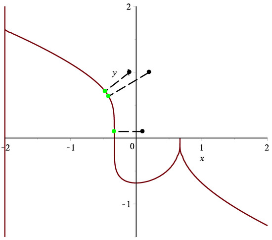
Figure 8. Graphic demonstration for Example 1.

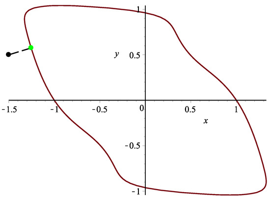
Example 2.

Assume a planar implicit curve $\Gamma :f(x,y)=x^6+4xy+2y^{18}-1=0$. Nine hundred test points from square $\left[-1.5,1.5\right]\times \left[-1.5,1.5\right]$ are taken. Algorithm 3 can rightly orthogonally project all 900 points onto planar implicit curve Γ. It satisfies the relationships $\left|f\left(p_{\Gamma }\right)\right|<{10}^{-10}$ and $\left|\left[(p-p_{\Gamma })\times \nabla f\left(p_{\Gamma }\right)\right]\right|<{10}^{-10}$. One test point $p=(-1.5,0.5)$ in this case is specified. Using Algorithm 3, the corresponding orthogonal projection point is $p_{\Gamma }$ = (−1.2539379406252056281, 0.57568037362837924613), and the initial iterative values $x_0$ are (−1.4,0.6), (−1.3,0.7), (−1.2,0.6), (−1.6,0.4), (−1.4,0.7), (−1.4,0.3), (−1.3,0.6), (−1.2,0.8), respectively. Each initial iterative value iterates 10 times, respectively, yielding 10 different iteration times in nanoseconds. In Table 7, the average running times of Algorithm 3 for eight different initial iterative values are 4,487,449, 4,202,203, 4,555,396, 4,533,326, 4,304,781, 4,163,107, 4,268,792 and 4,378,470 nanoseconds, respectively. In the end, the overall average running time is 4,361,691 nanoseconds (see Figure 9).

Table 7. Running times for different initial iterative values by Algorithm 3 in Example 2.

${\mathrm{x}}_0$ is the initial iterative point of Algorithm 3
${\mathrm{x}}_0$	(−1.4,0.6)	(−1.3,0.7)	(−1.2,0.6)	(−1.6,0.4)	(−1.4,0.7)	(−1.4,0.3)	(−1.3,0.6)	(−1.2,0.8)
1	4,811,297	4,626,018	4,902,396	4,431,627	4,115,036	4,326,372	4,130,822	4,859,314
2	4,505,727	3,912,778	4,665,879	4,242,339	4,503,391	4,278,999	4,288,241	3,866,268
3	4,124,334	4,230,176	5,060,009	4,460,799	3,869,937	4,283,195	4,155,043	4,619,351
4	4,147,473	4,609,361	4,243,387	4,869,970	4,167,195	4,007,433	4,147,670	4,774,583
5	4,440,814	3,617,951	4,384,258	4,852,657	4,593,295	4,297,552	4,611,293	4,125,097
6	4,227,363	4,138,344	3,966,863	4,783,579	3,902,268	4,248,232	3,897,182	4,835,741
7	4,449,021	4,153,901	4,847,488	4,902,842	4,580,368	4,147,208	4,134,164	3,991,250
8	4,646,411	4,189,724	4,474,738	4,309,208	4,296,653	4,219,366	4,481,757	4,285,602
9	5,092,419	4,263,006	4,759,462	4,358,871	4,220,163	3,850,277	4,496,335	4,347,691
10	4,429,635	4,280,772	4,249,480	4,121,366	4,799,502	3,972,433	4,345,415	4,079,804
Average	4,487,449	4,202,203	4,555,396	4,533,326	4,304,781	4,163,107	4,268,792	4,378,470
Total average	4,361,691

Figure 9. Graphic demonstration for Example 2.

The iterative error analysis for the test point p = (−1.5,0.5) under the same condition is presented in Table 8 with initial iterative points in the first row.

Table 8. The error analysis of the iteration process of Algorithm 3 in Example 2.

		(−1.4,0.6)		(−1.3,0.7)		(−1.6,0.4)		(−1.4,0.7)		(−1.3,0.6)		(−1.2,0.8)
Iterations	1	0.4693	1	0.46667	7	$1.438\times {10}^{-4}$	7	$1.598\times {10}^{-4}$	6	$1.450\times {10}^{-3}$	4	$5.603\times {10}^{-3}$
Iterations	3	0.2340	2	0.34342	8	$9.97\times {10}^{-6}$	8	$1.11\times {10}^{-5}$	8	$7.59\times {10}^{-6}$	5	$5.19\times {10}^{-4}$
Iterations	4	$8.47\times {10}^{-2}$	4	$9.06\times {10}^{-2}$	9	$6.83\times {10}^{-07}$	9	$7.61\times {10}^{-07}$	9	$5.20\times {10}^{-07}$	6	$3.70\times {10}^{-05}$
Iterations	6	$1.82\times {10}^{-3}$	5	$1.58\times {10}^{-2}$	10	$4.68\times {10}^{-08}$	10	$5.21\times {10}^{-08}$	10	$3.56\times {10}^{-08}$	7	$2.54\times {10}^{-06}$
Iterations	8	$9.78\times {10}^{-06}$	9	$7.42\times {10}^{-07}$	11	$3.20\times {10}^{-09}$	11	$3.57\times {10}^{-09}$	11	$2.44\times {10}^{-09}$	8	$1.74\times {10}^{-07}$
Iterations	12	$2.15\times {10}^{-10}$	11	$3.48\times {10}^{-09}$	12	$2.19\times {10}^{-10}$	12	$2.44\times {10}^{-10}$	12	$1.67\times {10}^{-10}$	10	$8.17\times {10}^{-10}$
Iterations	13	$1.47\times {10}^{-11}$	13	$1.63\times {10}^{-11}$	13	$1.50\times {10}^{-11}$	13	$1.67\times {10}^{-11}$	13	$1.14\times {10}^{-11}$	11	$5.60\times {10}^{-11}$
Iterations	14	$1.00\times {10}^{-12}$	14	$1.11\times {10}^{-12}$	14	$1.02\times {10}^{-12}$	14	$1.13\times {10}^{-12}$	14	$7.77\times {10}^{-13}$	12	$3.82\times {10}^{-12}$
Iterations	15	$6.01\times {10}^{-14}$	15	$6.74\times {10}^{-14}$	15	$6.35\times {10}^{-14}$	15	$7.14\times {10}^{-14}$	15	$4.52\times {10}^{-14}$	13	$2.54\times {10}^{-13}$
Iterations	16	$3.87\times {10}^{-15}$	16	$3.87\times {10}^{-15}$	16	$3.58\times {10}^{-15}$	16	$4.74\times {10}^{-15}$	16	$3.92\times {10}^{-15}$	14	$1.20\times {10}^{-14}$
Iterations	17	0	17	0	17	0	17	0	17	0	15	0

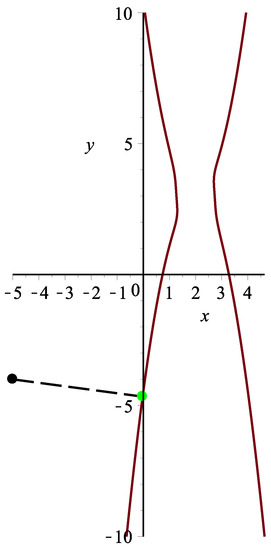
Example 3.

Assume a planar implicit curve $\Gamma :f(x,y)=12{(x-2)}^8+(x-2)(y-3)-{(y-3)}^4-1=0$. Three thousand and six hundred points from square $\left[0.0,4.0\right]\times \left[-3.0,6.0\right]$ are taken. Algorithm 3 can can orthogonally project all 3600 points onto planar implicit curve Γ. It satisfies the relationships $\left|f\left(p_{\Gamma }\right)\right|<{10}^{-10}$ and $\left|\left[(p-p_{\Gamma })\times \nabla f\left(p_{\Gamma }\right)\right]\right|<{10}^{-10}$. One test point $p=(-5.0,-4.0)$ in this case is specified. Using Algorithm 3, the corresponding orthogonal projection point is $p_{\Gamma }$ = (−0.027593939033081903,−4.6597845115690539), and the initial iterative values $x_0$ are (−12,−7), (−3,−5), (−5,−4), (−6.6,−9.9), (−2,−7), (−11,−6), (−5.6,−2.3), (−4.3,−5.7), respectively. Each initial iterative value iterates 10 times, respectively, yielding 10 different iteration times in nanoseconds. In Table 9, the average running times of Algorithm 3 for eight different initial iterative values are 299,569, 267,569, 290,719, 139,263, 125,962, 149,431, 289,643 and 124,885 nanoseconds, respectively. In the end, the overall average running time is 210,880 nanoseconds (see Figure 10).

Table 9. Running times for different initial iterative values by Algorithm 3 in Example 3.

${\mathrm{x}}_0$ is the initial iterative point of Algorithm 3
${\mathrm{x}}_0$	(−12,−7)	(−3,−5)	(−5,−4)	(−6.6,−9.9)	(−2,−7)	(−11,−6)	(−5.6,−2.3)	(−4.3,−5.7)
1	277,343	310,316	297,033	124,951	116,396	138,701	245,851	112,212
2	274,666	111,959	293,097	124,472	134,506	137,604	301,231	125,493
3	312,195	298,543	296,703	149,529	116,891	137,555	297,777	124,936
4	304,881	290,118	295,982	125,436	116,668	196,756	270,360	125,484
5	292,178	305,172	292,199	171,079	127,808	155,390	305,791	135,424
6	303,868	289,045	286,100	175,455	125,171	150,051	271,976	125,083
7	312,322	289,584	289,836	126,528	127,215	145,563	296,391	124,877
8	302,843	288,736	292,614	143,963	135,337	146,006	281,778	124,166
9	312,034	202,823	283,124	125,254	132,755	141,240	300,383	125,310
10	303,362	289,392	280,498	125,962	126,876	145,447	324,891	125,860
Average	299,569	267,569	290,719	139,263	125,962	149,431	289,643	124,885
Total average	210,880

Figure 10. Graphic demonstration for Example 3.

The iterative error analysis for the test point $\mathrm{p}=(-5,-4)$ under the same condition is presented in Table 10 with initial iterative points in the first row.

Table 10. The error analysis of the iteration process of Algorithm 3 in Example 3.

		(−3,−5)		(−2,−1)		(−1,−2)		(−2,−2)		(−2,−5)		(−1,−4)
Iterations	37	$1.36\times {10}^{-7}$	37	$1.18\times {10}^{-7}$	37	$1.48\times {10}^{-7}$	37	$1.37\times {10}^{-7}$	37	$1.36\times {10}^{-7}$	37	$1.29\times {10}^{-7}$
Iterations	38	$1.18\times {10}^{-7}$	38	$1.0\times {10}^{-7}$	38	$1.28\times {10}^{-7}$	38	$1.18\times {10}^{-7}$	38	$1.18\times {10}^{-7}$	38	$1.11\times {10}^{-7}$
Iterations	39	$1.0\times {10}^{-7}$	39	$8.43\times {10}^{-8}$	39	$1.10\times {10}^{-7}$	39	$1.01\times {10}^{-7}$	39	$1.0\times {10}^{-7}$	39	$9.43\times {10}^{-8}$
Iterations	40	$8.42\times {10}^{-8}$	40	$6.94\times {10}^{-8}$	40	$9.34\times {10}^{-8}$	40	$8.45\times {10}^{-8}$	40	$8.41\times {10}^{-8}$	40	$7.86\times {10}^{-8}$
Iterations	41	$6.93\times {10}^{-8}$	41	$5.55\times {10}^{-8}$	41	$7.79\times {10}^{-8}$	41	$6.96\times {10}^{-8}$	41	$6.93\times {10}^{-8}$	41	$6.41\times {10}^{-8}$
Iterations	42	$5.54\times {10}^{-8}$	42	$4.27\times {10}^{-8}$	42	$6.34\times {10}^{-8}$	42	$5.57\times {10}^{-8}$	42	$5.54\times {10}^{-8}$	42	$5.07\times {10}^{-8}$
Iterations	43	$4.26\times {10}^{-8}$	43	$3.08\times {10}^{-8}$	43	$5.0\times {10}^{-8}$	43	$4.29\times {10}^{-8}$	43	$4.26\times {10}^{-8}$	43	$3.82\times {10}^{-8}$
Iterations	44	$3.07\times {10}^{-8}$	44	$1.98\times {10}^{-8}$	44	$3.76\times {10}^{-8}$	44	$3.1\times {10}^{-8}$	44	$3.07\times {10}^{-8}$	44	$2.67\times {10}^{-8}$
Iterations	45	$1.97\times {10}^{-8}$	45	$9.56\times {10}^{-9}$	45	$2.61\times {10}^{-8}$	45	$5.89\times {10}^{-9}$	45	$1.97\times {10}^{-8}$	45	$1.59\times {10}^{-9}$
Iterations	46	$9.49\times {10}^{-9}$	46	$6.11\times {10}^{-11}$	46	$1.54\times {10}^{-8}$	46	$9.71\times {10}^{-10}$	46	$9.49\times {10}^{-9}$	46	$5.97\times {10}^{-10}$
Iterations	47	$1.78\times {10}^{-15}$	47	$2.43\times {10}^{-11}$	47	$5.48\times {10}^{-9}$	47	$2.03\times {10}^{-12}$	47	$1.31\times {10}^{-12}$	47	$3.79\times {10}^{-12}$
Iterations	48	0	48	0	48	0	48	0	48	0	48	0

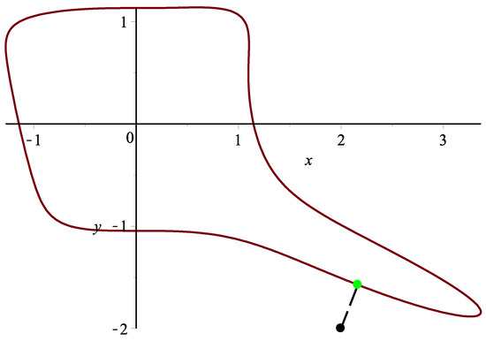
Example 4.

Assume a planar implicit curve $\Gamma :f(x,y)=x^6+2x^{5}y-2x^3{y}^2+x^4-y^3+2y^8-4=0$. Two thousand one hundred test points from the square $\left[-2.0,4.0\right]\times \left[-2.0,1.5\right]$ are taken. Algorithm 3 can orthogonally project all 2100 points onto planar implicit curve Γ. It satisfies the relationships $\left|f\left(p_{\Gamma }\right)\right|<{10}^{-10}$ and $\left|\left[(p-p_{\Gamma })\times \nabla f\left(p_{\Gamma }\right)\right]\right|<{10}^{-10}$. One test point $p=(2.0,-2.0)$ in this case is specified. Using Algorithm 3, the corresponding orthogonal projection point is $p_{\Gamma }$ = (2.1654788271485294, −1.5734131236664724), and the initial iterative values $x_0$ are (2.2,−2.1), (2.3,−1.9), (2.4,−1.8), (2.1,−2.3), (2.4,−1.6), (2.3,−1), (1.6,−2.5), (2.6,−2.5), respectively. Each initial iterative value iterates 10 times, respectively, yielding 10 different iteration times in nanoseconds. In Table 11, the average running times of Algorithm 3 for eight different initial iterative values are 403,539, 442,631, 395,384, 253,156, 241,510, 193,592, 174,340 and 187,362 nanoseconds, respectively. In the end, the overall average running time is 286,439 nanoseconds (see Figure 11).

Table 11. Running times for different initial iterative values by Algorithm 3 in Example 4.

${\mathrm{x}}_0$ is the initial iterative point of Algorithm 3
${\mathrm{x}}_0$	(2.2,−2.1)	(2.3,−1.9)	(2.4,−1.8)	(2.1,−2.3)	(2.4,−1.6)	(2.3,−1)	(1.6,−2.5)	(2.6,−2.5)
1	430,112	740,948	421,825	254,230	260,450	172,025	180,110	115,138
2	404,301	406,073	420,653	253,648	221,176	198,725	179,517	187,424
3	426,059	429,215	354,579	207,810	249,507	171,104	179,836	210,163
4	412,996	372,201	420,155	252,192	260,296	169,377	179,735	198,288
5	349,826	407,902	420,748	254,064	169,470	256,737	136,947	194,841
6	412,088	422,447	433,176	316,291	249,825	187,722	149,392	195,673
7	413,990	410,384	453,070	253,329	249,704	176,733	198,042	188,232
8	454,218	409,190	314,484	251,488	248,592	170,296	180,078	194,450
9	425,873	418,357	357,542	236,264	249,482	252,598	179,940	194,180
10	305,927	409,593	357,610	252,244	256,600	180,605	179,806	195,230
Average	403,539	442,631	395,384	253,156	241,510	193,592	174,340	187,362
Total average	286,439

Figure 11. Graphic demonstration for Example 4.

The iterative error analysis for the test point $\mathrm{p}=(2,-2)$ under the same condition is presented in Table 12 with initial iterative points in the first row.

Table 12. The error analysis of the iteration process of Algorithm 3 in Example 4.

		(2.2,−2.1)		(2.3,−1.9)		(2.1,−2.3)		(2.4,−1.6)		(1.6,−2.5)		(2.6,−2.5)
Iterations	5	$7.42\times {10}^{-6}$	3	$1.42\times {10}^{-4}$	4	$1.65\times {10}^{-4}$	4	$4.29\times {10}^{-5}$	4	$2.21\times {10}^{-4}$	4	$1.45\times {10}^{-4}$
Iterations	6	$6.41\times {10}^{-7}$	4	$1.22\times {10}^{-5}$	5	$1.23\times {10}^{-6}$	5	$3.70\times {10}^{-6}$	5	$1.90\times {10}^{-5}$	5	$1.25\times {10}^{-5}$
Iterations	7	$5.53\times {10}^{-8}$	5	$1.05\times {10}^{-6}$	6	$1.06\times {10}^{-7}$	6	$3.20\times {10}^{-7}$	6	$1.64\times {10}^{-6}$	6	$1.08\times {10}^{-6}$
Iterations	8	$4.7\times {10}^{-9}$	6	$9.12\times {10}^{-8}$	7	$9.19\times {10}^{-9}$	7	$2.76\times {10}^{-8}$	7	$1.41\times {10}^{-7}$	7	$9.34\times {10}^{-8}$
Iterations	9	$4.12\times {10}^{-10}$	7	$7.87\times {10}^{-9}$	8	$7.94\times {10}^{-10}$	8	$2.38\times {10}^{-9}$	8	$1.22\times {10}^{-8}$	8	$8.07\times {10}^{-9}$
Iterations	10	$3.56\times {10}^{-11}$	8	$6.80\times {10}^{-10}$	9	$6.85\times {10}^{-11}$	9	$2.06\times {10}^{-10}$	9	$1.05\times {10}^{-9}$	9	$6.96\times {10}^{-10}$
Iterations	11	$3.05\times {10}^{-12}$	9	$5.87\times {10}^{-11}$	10	$5.89\times {10}^{-12}$	10	$1.78\times {10}^{-11}$	10	$9.13\times {10}^{-11}$	10	$6.01\times {10}^{-11}$
Iterations	12	$2.39\times {10}^{-13}$	10	$5.04\times {10}^{-12}$	11	$4.87\times {10}^{-13}$	11	$1.56\times {10}^{-12}$	11	$7.85\times {10}^{-12}$	11	$5.17\times {10}^{-12}$
Iterations	13	$1.89\times {10}^{-15}$	11	$4.15\times {10}^{-13}$	12	$2.20\times {10}^{-14}$	12	$1.58\times {10}^{-13}$	12	$6.51\times {10}^{-13}$	12	$4.25\times {10}^{-13}$
Iterations	14	$2.12\times {10}^{-16}$	12	$1.53\times {10}^{-14}$	13	$4.71\times {10}^{-16}$	13	$3.56\times {10}^{-14}$	13	$3.37\times {10}^{-14}$	13	$1.61\times {10}^{-14}$
Iterations	15	0	13	0	14	0	14	0	14	0	14	0

Example 5.

Assume a planar implicit curve $\Gamma :f(x,y)=x^{15}+2x^{5}y-2x^3{y}^2+x^4-y^3-4y^{18}-4=0$. Tow thousand four hundred test points from the square $\left[0,3\right]\times \left[-3,3\right]$ are taken. Algorithm 3 can orthogonally project all 2400 points onto planar implicit curve Γ. It satisfies the relationships $\left|f\left(p_{\Gamma }\right)\right|<{10}^{-10}$ and $\left|\left[(p-p_{\Gamma })\times \nabla f\left(p_{\Gamma }\right)\right]\right|<{10}^{-10}$.

One test point $\mathrm{p}=(12,-20)$ in this case is specified. Using Algorithm 3, the corresponding orthogonal projection point is ${\mathrm{p}}_{\Gamma }$ = (16.9221067487652, −9.77831982969495), and the initial iterative values ${\mathrm{x}}_0$ are (12,−20), (3,−5), (5,−4), (66,−99), (14,−21), (11,−6), (56,−23), (13,−7), respectively. Each initial iterative value iterates 10 times, respectively, yielding 10 different iteration times in nanoseconds. In Table 13, the average running times of Algorithm 3 for eight different initial iterative values are 285,449, 447,036, 405,726, 451,383, 228,491, 208,624, 410,489 and 224,141 nanoseconds, respectively. In the end, the overall average running time is 332,667 nanoseconds (see Figure 12).

Table 13. Running times for different initial iterative values by Algorithm 3 in Example 5.

${\mathrm{x}}_0$ is the initial iterative point of Algorithm 3
${\mathrm{x}}_0$	(12,−20)	(3,−5)	(5,−4)	(66,−99)	(14,−21)	(11,−6)	(56,−23)	(13,−7)
1	248,703	449,007	234,127	485,542	236,887	262,514	441,322	217,746
2	323,108	448,493	442,871	406,267	262,696	217,260	449,011	217,915
3	247,861	456,350	418,751	467,633	259,544	198,615	418,260	217,787
4	284,727	448,722	465,808	458,852	138,867	217,176	476,528	217,776
5	321,696	444,663	403,970	466,525	237,369	189,288	414,269	211,879
6	320,798	451,849	450,119	465,345	138,523	265,633	418,683	241,267
7	327,936	448,836	321,268	417,030	266,929	217,299	413,880	217,836
8	321,471	435,693	465,314	445,768	239,203	161,549	482,363	217,234
9	147,980	449,984	398,126	446,046	267,621	239,762	415,523	241,129
10	310,207	436,765	456,906	454,822	237,269	117,144	175,049	240,841
Average	285,449	447,036	405,726	451,383	228,491	208,624	410,489	224,141
Total Average	332,667

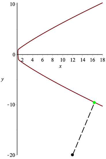
Figure 12. Graphic demonstration for Example 5.

The iterative error analysis for the test point $\mathrm{p}=(12,-20)$ under the same condition is presented in Table 14 with initial iterative points in the first row.

Table 14. The error analysis of the iteration process of Algorithm 3 in Example 5.

		(12,−20)		(3,−5)		(66,−99)		(5,−4)		(56,−23)		(13,−7)
Iterations	7	$3.42\times {10}^{-3}$	10	$3.32\times {10}^{-3}$	15	$3.25\times {10}^{-3}$	15	$3.22\times {10}^{-3}$	23	$4.68\times {10}^{-3}$	1	$3.09\times {10}^{-3}$
Iterations	8	$3.05\times {10}^{-3}$	11	$2.95\times {10}^{-3}$	16	$2.88\times {10}^{-3}$	16	$2.85\times {10}^{-3}$	24	$4.65\times {10}^{-3}$	2	$3.34\times {10}^{-4}$
Iterations	9	$2.68\times {10}^{-3}$	12	$2.59\times {10}^{-3}$	17	$2.52\times {10}^{-3}$	17	$2.49\times {10}^{-3}$	25	$4.62\times {10}^{-3}$	3	0
Iterations	10	$2.33\times {10}^{-3}$	13	$2.24\times {10}^{-3}$	18	$2.17\times {10}^{-3}$	18	$2.14\times {10}^{-3}$	26	$4.58\times {10}^{-3}$
Iterations	11	$1.98\times {10}^{-3}$	14	$1.89\times {10}^{-3}$	19	$1.82\times {10}^{-3}$	19	$1.79\times {10}^{-3}$	27	$4.55\times {10}^{-3}$
Iterations	12	$1.63\times {10}^{-3}$	15	$1.54\times {10}^{-3}$	20	$1.48\times {10}^{-3}$	20	$1.45\times {10}^{-3}$	28	$4.52\times {10}^{-3}$
Iterations	13	$1.29\times {10}^{-3}$	16	$1.21\times {10}^{-3}$	21	$1.14\times {10}^{-3}$	21	$1.12\times {10}^{-3}$	29	$4.48\times {10}^{-3}$
Iterations	14	$9.62\times {10}^{-4}$	17	$8.77\times {10}^{-4}$	22	$8.13\times {10}^{-4}$	22	$7.89\times {10}^{-4}$	30	$4.45\times {10}^{-3}$
Iterations	15	$6.35\times {10}^{-4}$	18	$5.52\times {10}^{-4}$	23	$4.89\times {10}^{-4}$	23	$4.66\times {10}^{-4}$	31	$4.42\times {10}^{-3}$
Iterations	16	$3.15\times {10}^{-5}$	19	$2.33\times {10}^{-4}$	24	$1.71\times {10}^{-4}$	24	$1.49\times {10}^{-4}$	32	$4.39\times {10}^{-4}$
Iterations	17	0	20	$8.04\times {10}^{-5}$	25	$1.41\times {10}^{-5}$	25	$1.63\times {10}^{-5}$	33	$4.36\times {10}^{-5}$

Example 6.

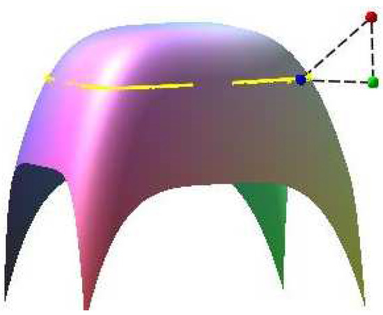
Assume a planar implicit curve $\Gamma :f(x,y)=-(x^6+2y^4-4)=0$. One spatial test point $p^{\prime }=(2.0,1.5,5)$ in this case is specified, and orthogonally project it onto plane $x-y$, so the planar test point will be $p=(2.0,1.5)$. Using Algorithm 3, the corresponding orthogonal projection point on plane $x-y$ is $p_{\Gamma }=(1.1436111944138613,0.96895628133918197)$, and it satisfies the two relationships $\left|f\left(x_{n+1}\right)\right|<1.2\times {10}^{-14}$ and $\left|⟨p-x_{n+1},t⟩\right|<1.2\times {10}^{-15}$. In the iterative error Table 15, six points (1,1), (1.5,1.5), (−1,1), (1,−1), (1.5,1), (1,1.5) in the first row are the initial iterative points $x_0$ of Algorithm 3. In Figure 13, red, green and blue points are the spatial test point, planar test point and their common corresponding orthogonal projection point, respectively. Assume surface $z=f(x,y)$ with two free variables x and y. The yellow curve is planar implicit curve $f(x,y)=0$.

Table 15. The error analysis of the iteration process of Algorithm 3 in Example 6.

		(1,1)		(−1.1,1.5)		(−1,1)		(1,−1)		(−1.5,1)		(1,1.5)
Iterations	1	$3.03\times {10}^{-3}$	2	$1.01\times {10}^{-2}$	1	3.95	1	$8.67\times {10}^{-1}$	4	$3.53\times {10}^{-4}$	1	$2.03\times {10}^{-1}$
Iterations	2	$1.21\times {10}^{-7}$	3	$1.06\times {10}^{-8}$	2	3.37	2	$2.72\times {10}^{-1}$	5	$2.78\times {10}^{-5}$	2	$4.71\times {10}^{-3}$
Iterations	3	$6.22\times {10}^{-11}$	4	$8.82\times {10}^{-10}$	3	3.85	3	$1.21\times {10}^{-2}$	6	$2.18\times {10}^{-6}$	3	$2.38\times {10}^{-8}$
Iterations	4	$1.52\times {10}^{-11}$	5	$2.16\times {10}^{-10}$	4	1.00	4	$2.20\times {10}^{-6}$	7	$1.70\times {10}^{-7}$	4	$3.84\times {10}^{-11}$
Iterations	5	$5.58\times {10}^{-13}$	6	$6.04\times {10}^{-11}$	5	$3.80\times {10}^{-1}$	5	$1.34\times {10}^{-11}$	8	$1.33\times {10}^{-8}$	5	$1.07\times {10}^{-11}$
Iterations	6	$1.34\times {10}^{-13}$	7	$4.74\times {10}^{-12}$	6	$3.14\times {10}^{-2}$	6	$3.30\times {10}^{-12}$	9	$1.04\times {10}^{-9}$	6	$8.30\times {10}^{-13}$
Iterations	7	$4.56\times {10}^{-14}$	8	$3.82\times {10}^{-13}$	7	$2.37\times {10}^{-5}$	7	$9.36\times {10}^{-13}$	10	$8.20\times {10}^{-11}$	7	$5.36\times {10}^{-14}$
Iterations	8	0	9	$4.13\times {10}^{-14}$	8	$6.56\times {10}^{-12}$	8	$8.46\times {10}^{-14}$	11	$5.62\times {10}^{-12}$	8	$7.04\times {10}^{-15}$
Iterations			10	$1.45\times {10}^{-14}$	9	$8.74\times {10}^{-13}$	9	$1.79\times {10}^{-14}$	12	0	9	0
Iterations			11	$1.23\times {10}^{-14}$	10	$7.97\times {10}^{-14}$	10	0
Iterations			12	0	11	0

Figure 13. Graphic demonstration for Example 6.

Remark 4.

In the 22 tables, all computations were done by using g++ in the Fedora Linux 8 environment. The iterative termination criteria ${\epsilon }_1$ for Algorithm 1 and Algorithm 2 are ${\epsilon }_1={10}^{-7}$ and ${\epsilon }_2={10}^{-15}$, respectively. Examples 1–6 are computed using a personal computer with Intel i7-4700 3.2-GHz CPU and 4.0 GB memory.

In Examples 2–6, if the degree of every planar implicit curve is more than five, it is difficult to get the intersection between the line segment determined by test point p and ${\mathrm{p}}^{+}$ and the planar implicit curve by using the circle shrinking algorithm in [14]. The running time comparison for Algorithm in [14] was not done, and it was not done for the circle double-and-bisect algorithm in [36] due to the same reason. The running time comparison test by using the circle double-and-bisect algorithm in [36] has not been done because it is difficult to solve the intersection between the circle and the planar implicit curve by using the circle double-and-bisect algorithm. In addition, many methods (Newton’s method, the geometrically-motivated method [31,32], the osculating circle algorithm [33], the Bézer clipping method [25,26,27], etc.) cannot guarantee complete convergence for Examples 2–5. The running time comparison test for those methods in [25,26,27,31,32,33] has not been done yet. From Table 2 in [36], the circle shrinking algorithm in [14] is faster than the existing methods, while Algorithm 3 is faster than the circle shrinking algorithm in [14] in our Example 1. Then, Algorithm 3 is faster than the existing methods. Furthermore, Algorithm 3 is more robust and efficient than the existing methods.

Besides, it is not difficult to find that if test point p is close to the planar implicit curve and initial iterative point ${\mathrm{x}}_0$ is close to the test point p, for a lower degree of and fewer terms in the planar implicit curve and lower precision of the iteration, Algorithm 3 will use less total average running time. Otherwise, Algorithm 3 will use more time.

Remark 5.

Algorithm 3 essentially makes an orthogonal projection of test point onto a planar implicit curve $\Gamma :f\left(x\right)=0$. For the multiple orthogonal points situation, the basic idea of the authors’ approach is as follows:

(1) 

Divide a planar region $\left[a,b\right]\times \left[c,d\right]$ of planar implicit curve into $m^2$ sub-regions $\left[a_i,a_{i+1}\right]\times \left[c_j,c_{j+1}\right],i,j=0,1,2,\dots ,m-1$, where $a=a_0,a_{i+1}-a_i=\frac{b-a}{m},b=a_m,c=c_0,c_{j+1}-c_j=\frac{d-c}{m},d=c_m$.

(2) 

Randomly select an initial iterative value in each sub-region.

(3) 

Using Algorithm 3 and using each initial iterative value, do the iteration, respectively. Let us assume that the corresponding orthogonal projection points are $p_{{\Gamma }_{ij}},i,j=0,1,2,\dots ,m-1$, respectively.

(4) 

Compute the local minimum distances $d_{ij},i,j=0,1,2,\dots ,m-1$, where $d_{ij}=∥p-p_{{\Gamma }_{ij}}∥$.

(5) 

Compute the global minimum distance $d=∥p-f\left(p_{\Gamma }\right)∥=min\{d_{ij}\},i,j=0,1,2,\dots ,m-1$.

To find as many solutions as possible, a larger value of m is taken.

Remark 6.

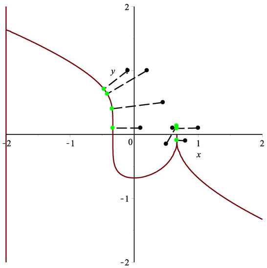
In Example 1, for the test points (−0.1,1.0), (0.2,1.0), (0.1,0.1), (0.45,0.5), by using Algorithm 3, the corresponding orthogonal projection points $p_{\Gamma }$ are $(-0.47144354751227009,0.70879213227958752)$, $(-0.42011639143389254,0.63408011508207950)$, $(-0.33334322619432892,0.099785192603767206)$, $(-0.34352305539212918$,$0.401230229163152532)$, respectively (see Figure 14 and Table 16). In addition to the six test examples, many other examples have also been tested. According to these results, if test point p is close to the planar implicit curve $f\left(x\right)$, for different initial iterative values $x_0$, which are also close to the corresponding orthogonal projection point $p_{\Gamma }$, it can converge to the corresponding orthogonal projection point $p_{\Gamma }$ by using Algorithm 3, namely the test point p and its corresponding orthogonal projection point $p_{\Gamma }$ satisfy the inequality relationships:

$$\left\{\begin{array}{c}\left|f\left(p_{\Gamma }\right)\right|<{10}^{-10},\hfill \\ \left|\left[(p-p_{\Gamma })\times \nabla f\left(p_{\Gamma }\right)\right]\right|<{10}^{-10}.\hfill \end{array}\right.$$

(42)

Figure 14. Graphic demonstration for the singular point case of Algorithm 3.

Table 16. Distance for the singular point case of Algorithm 3.

Test point p	Initial iterative point ${\mathrm{x}}_0$	Distance in [14]	Distance in [36]	Distance by ours
(−0.1,1)	(−0.5,0.9)	0.471990	0.471988	0.47198763883259622
(0.2,1)	(−0.6,0.6)	0.720032	0.720030	0.72002895851718132
(0.1,0.1)	(−0.2,0.2)	0.433352	0.433345	0.43334327943413038
(0.45,0.5)	(−0.2,0.5)		0.549262	0.79964636375714451
(1.0,0.01)	(0.6,0.01)			0.32956742971206581
(0.6,0.1)	(0.5,0.01)			0.063752646448070471
(0.5,−0.15)	(0.55,−0.2)			0.16628421658831499
(0.8,−0.1)	(0.75,−0.1)			0.13613197908773955

Thus, it illustrates that the convergence of Algorithm 3 is independent of the initial value and Algorithm 3 is efficient. In sum, the algorithm can meet the top two of the ten challenges proposed by Professor Les A. Piegl [41] in terms of robustness and efficiency.

Remark 7.

From the authors’ six test examples, Algorithm 3 is robust and efficient. If test point p is very far away from the planar implicit curve and the degree of the planar implicit curve is very high, Algorithm 3 also converges. However, inequality relationships (42) could not be satisfied simultaneously. In addition, if the planar implicit curve contains singular points, Algorithm 3 only works for test point p in a suitable position. Namely, for any initial iterative point $x_0$, test point p can be orthogonally projected onto the planar implicit curve, but with a larger distance $∥p-p_{\Gamma }∥$ than the minimum distance $∥p-p_s∥$ between the test point and the orthogonal projection point, where $p_s$ is the singular point. For example, for the test point (1.0,0.01), (0.6,0.1), (0.5,−0.15), (0.8,−0.1), Algorithm 3 gives the corresponding orthogonal projection points $p_{\Gamma }$ as $(0.66370473801453017,0.092784537693334545)$, $(0.66704812931370775,0.097528910436113817)$, $(0.663704738014530,0.13435089298485379)$, $(0.66418591136724639,-0.090702201378858334)$, respectively. However, the actual corresponding orthogonal projection point of four test points is $(0.66666666666666667,0.0)$ (see Figure 14 and Table 16).

Remark 8.

This remark is added to numerically validate the convergence order of two, thanks to the reviewers’ insightful comments, which corrects the previous wrong calculation of the convergence order. The iterative error ratios for the test point p = $(-0.1,1.0)$ in Example 1 are presented in Table 17 with initial iterative points in the first row. The formula $\left|ln\left(\frac{\sqrt{⟨x_{n+1}-p_{\Gamma },x_{n+1}-p_{\Gamma }⟩}}{\sqrt{⟨x_n-p_{\Gamma },x_n-p_{\Gamma }⟩}}\right)\right|$ is used to compute error ratios for each iteration in rows other than the first one, which is the same for Table 18, Table 19, Table 20, Table 21 and Table 22. From the six tables, once again combined with the order of convergence formula $\rho \approx \left|\frac{ln\left(\sqrt{⟨x_{n+1}-p_{\Gamma },x_{n+1}-p_{\Gamma }⟩}/\sqrt{⟨x_n-p_{\Gamma },x_n-p_{\Gamma }⟩}\right)}{ln\left(\sqrt{⟨x_n-p_{\Gamma },x_n-p_{\Gamma }⟩}/\sqrt{⟨x_{n-1}-p_{\Gamma },x_{n-1}-p_{\Gamma }⟩}\right)}\right|$, it is not difficult to find out that the order of convergence for each example is approximately between one and two, which verifies Theorem 1. The convergence formula ρ comes from the Formula [42], i.e., ${\displaystyle \rho \approx \frac{ln\left|\left(x_{n+1}-\alpha \right)/\left(x_n-\alpha \right)\right|}{ln\left|\left(x_n-\alpha \right)/\left(x_{n-1}-\alpha \right)\right|}}$.

Table 17. The error ratios for each iteration in Example 1 of Algorithm 3.

		(−0.1,0.8)		(−0.1,0.9)		(−0.2,0.8)		(−0.3,1.1)		(−0.3,1.0)		(−0.4,1.1)
Iterations	1	5.6	1	7.05	1	6.33	1	7.55	1	7.55	1	6.38
Iterations	2	6.97	2	8.42	2	7.69	2	8.92	2	8.92	2	7.75
Iterations	3	8.34	3	9.79	3	9.06	3	10.3	3	10.3	3	9.11
Iterations	4	9.71	4	11.2	4	10.4	4	11.7	4	11.7	4	10.5
Iterations	5	11.1	5	12.5	5	11.8	5	13.0	5	13.0	5	11.8
Iterations	6	12.4	6	13.9	6	13.2	6	14.4	6	14.4	6	13.2
Iterations	7	13.8	7	15.3	7	14.5	7	15.7	7	15.7	7	14.6
Iterations	8	15.2	8	16.7	8	15.9	8	17.0	8	17.0	8	15.9
Iterations	9	16.6	9	18.3	9	17.4	9	18.1	9	18.1	9	17.2
Iterations	10	18.2	10	21.8	10	19.4					10	18.2

Table 18. The error ratios for each iteration in Example 2 of Algorithm 3.

		(−1.4,0.6)		(−1.3,0.7)		(−1.6,0.4)		(−1.4,0.7)		(−1.3,0.6)		(−1.2,0.8)
Iterations	1	3.032	1	2.743	1	1.258	1	6.052	1	4.324	1	3.032
Iterations	2	7.816	2	7.234	2	3.891	2	11.26	2	10.41	2	7.819
Iterations	3	2.539	3	5.801	3	9.538	3		3		3	3.060

Table 19. The error ratios for each iteration in Example 3 of Algorithm 3.

		$(-3,-5)$		$(-2,-1)$		$(-1,-2)$		$(-2,-2)$		$(-2,-5)$		$(-1,-4)$
Iterations	1	$4.81\times {10}^{-2}$	1	$4.81\times {10}^{-2}$	1	$4.81\times {10}^{-2}$	1	$4.81\times {10}^{-2}$	1	$4.81\times {10}^{-2}$	1	$4.81\times {10}^{-2}$
Iterations	2	$2.81\times {10}^{-2}$	2	$2.81\times {10}^{-2}$	2	$2.81\times {10}^{-2}$	2	$2.81\times {10}^{-2}$	2	$2.81\times {10}^{-2}$	2	$2.81\times {10}^{-2}$
Iterations	3	$1.67\times {10}^{-2}$	3	$1.67\times {10}^{-2}$	3	$1.67\times {10}^{-2}$	3	$1.67\times {10}^{-2}$	3	$1.67\times {10}^{-2}$	3	$1.67\times {10}^{-2}$
Iterations	4	$9.97\times {10}^{-3}$	4	$9.97\times {10}^{-3}$	4	$9.98\times {10}^{-3}$	4	$9.97\times {10}^{-3}$	4	$9.97\times {10}^{-3}$	4	$9.98\times {10}^{-3}$
Iterations	5	$9.0\times {10}^{-3}$	5	$9.0\times {10}^{-3}$	5	$9.0\times {10}^{-3}$	5	$9.0\times {10}^{-3}$	5	$9.0\times {10}^{-3}$	5	$9.0\times {10}^{-3}$
Iterations	6	$3.62\times {10}^{-3}$	6	$3.62\times {10}^{-3}$	6	$3.62\times {10}^{-3}$	6	$3.62\times {10}^{-3}$	6	$3.62\times {10}^{-3}$	6	$3.62\times {10}^{-3}$
Iterations	7	$2.19\times {10}^{-3}$	7	$2.19\times {10}^{-3}$	7	$2.19\times {10}^{-3}$	7	$2.19\times {10}^{-3}$	7	$2.19\times {10}^{-3}$	7	$2.19\times {10}^{-3}$
Iterations	8	$1.32\times {10}^{-3}$	8	$1.32\times {10}^{-3}$	8	$1.32\times {10}^{-3}$	8	$1.32\times {10}^{-3}$	8	$1.32\times {10}^{-3}$	8	$1.32\times {10}^{-3}$
Iterations	9	$8.01\times {10}^{-4}$	9	$8.01\times {10}^{-4}$	9	$8.01\times {10}^{-4}$	9	$8.01\times {10}^{-4}$	9	$8.01\times {10}^{-4}$	9	$8.01\times {10}^{-4}$
Iterations	10	$4.85\times {10}^{-4}$	10	$4.85\times {10}^{-4}$	10	$4.85\times {10}^{-4}$	10	$4.85\times {10}^{-4}$	10	$4.85\times {10}^{-4}$	10	$4.85\times {10}^{-4}$

Table 20. The error ratios for each iteration in Example 4 of Algorithm 3.

		$(2.2,-2.1)$		$(2.3,-1.9)$		$(2.1,-2.3)$		$(2.4,-1.6)$		$(1.6,-2.5)$		$(2.6,-2.5)$
Iterations	1	0.6782	1	0.6779	1	0.6785	1	0.6776	1	0.6794	1	0.677
Iterations	2	1.356	2	1.356	2	1.355	2	1.356	2	1.355	2	1.356
Iterations	3	1.356			3	1.356	3	1.356	3	1.356	3	1.356
Iterations	4	1.356			4	1.356	4	1.356	4	1.356	4	1.356
Iterations	5	1.356			5	1.356	5	1.356	5	1.356	5	1.356
Iterations					6	1.356			6	1.356	6	1.356

Table 21. The error ratios for each iteration in Example 5 of Algorithm 3.

		(12,−20)		(3,−5)		(66,−99)		(5,−4)		(56,−23)		(13,−7)
Iterations	8	$1.64\times {10}^{-2}$	11	$1.64\times {10}^{-2}$	16	$1.64\times {10}^{-2}$	16	$1.64\times {10}^{-2}$	24	$1.26\times {10}^{-2}$	1	$8.99\times {10}^{-3}$
Iterations	9	$1.64\times {10}^{-2}$	12	$1.64\times {10}^{-2}$	17	$1.64\times {10}^{-2}$	17	$1.64\times {10}^{-2}$	25	$1.26\times {10}^{-2}$	2	$1.59\times {10}^{-2}$
Iterations	10	$1.64\times {10}^{-2}$	13	$1.64\times {10}^{-2}$	18	$1.64\times {10}^{-2}$	18	$1.64\times {10}^{-2}$	26	$1.27\times {10}^{-2}$
Iterations	11	$1.64\times {10}^{-2}$	14	$1.63\times {10}^{-2}$	19	$1.63\times {10}^{-2}$	19	$1.63\times {10}^{-2}$	27	$1.27\times {10}^{-2}$
Iterations	12	$1.63\times {10}^{-2}$	15	$1.63\times {10}^{-2}$	20	$1.63\times {10}^{-2}$	20	$1.63\times {10}^{-2}$	28	$1.27\times {10}^{-2}$
Iterations	13	$1.63\times {10}^{-2}$	16	$1.63\times {10}^{-2}$	21	$1.63\times {10}^{-2}$	21	$1.63\times {10}^{-2}$	29	$1.27\times {10}^{-2}$
Iterations	14	$1.63\times {10}^{-2}$	17	$1.63\times {10}^{-2}$	22	$1.63\times {10}^{-2}$	22	$1.63\times {10}^{-2}$	30	$1.28\times {10}^{-2}$
Iterations	15	$1.63\times {10}^{-2}$	18	$1.62\times {10}^{-2}$	23	$1.62\times {10}^{-2}$	23	$1.62\times {10}^{-2}$	31	$1.28\times {10}^{-2}$
Iterations	16	$1.62\times {10}^{-2}$	19	$1.62\times {10}^{-2}$	24	$1.62\times {10}^{-2}$	24	$1.62\times {10}^{-2}$	32	$1.28\times {10}^{-2}$
Iterations	17	$1.62\times {10}^{-2}$	20	$1.62\times {10}^{-2}$	25	$1.62\times {10}^{-2}$	25	$1.62\times {10}^{-2}$	33	$1.28\times {10}^{-2}$

Table 22. The error ratios for each iteration in Example 6 of Algorithm 3.

		(1,1)		(−1.1,1.5)		(−1,1)		(1,−1)		(−1.5,1)		(1,1.5)
Iterations	1	$6.69\times {10}^{-1}$	6	$6.69\times {10}^{-1}$	9	$6.69\times {10}^{-1}$	13	$6.69\times {10}^{-1}$	23	$6.69\times {10}^{-1}$	5	$6.69\times {10}^{-1}$
Iterations	2	$6.69\times {10}^{-1}$	7	$6.69\times {10}^{-1}$	10	$6.69\times {10}^{-1}$	14	$6.69\times {10}^{-1}$	24	$6.69\times {10}^{-1}$	6	$6.69\times {10}^{-1}$
Iterations	3	$6.69\times {10}^{-1}$	8	$6.69\times {10}^{-1}$	11	$6.69\times {10}^{-1}$	15	$6.69\times {10}^{-1}$	25	$6.69\times {10}^{-1}$	7	$6.69\times {10}^{-1}$
Iterations	4	$6.69\times {10}^{-1}$	9	$6.69\times {10}^{-1}$	12	$6.69\times {10}^{-1}$	16	$6.69\times {10}^{-1}$	26	$6.69\times {10}^{-1}$	8	$6.69\times {10}^{-1}$
Iterations	5	$6.69\times {10}^{-1}$	10	$6.69\times {10}^{-1}$	13	$6.69\times {10}^{-1}$	17	$6.69\times {10}^{-1}$	27	$6.69\times {10}^{-1}$	9	$6.69\times {10}^{-1}$
Iterations	6	$6.69\times {10}^{-1}$	11	$6.69\times {10}^{-1}$	14	$6.69\times {10}^{-1}$	18	$6.69\times {10}^{-1}$	28	$6.69\times {10}^{-1}$	10	$6.69\times {10}^{-1}$
Iterations	7	$6.69\times {10}^{-1}$	12	$6.69\times {10}^{-1}$	15	$6.69\times {10}^{-1}$	19	$6.69\times {10}^{-1}$	29	$6.69\times {10}^{-1}$	11	$6.69\times {10}^{-1}$
Iterations	8	$6.69\times {10}^{-1}$	13	$6.69\times {10}^{-1}$	16	$6.69\times {10}^{-1}$	20	$6.69\times {10}^{-1}$	30	$6.69\times {10}^{-1}$	12	$6.69\times {10}^{-1}$
Iterations	9	$6.69\times {10}^{-1}$	14	$6.69\times {10}^{-1}$	17	$6.69\times {10}^{-1}$	21	$6.69\times {10}^{-1}$	31	$6.69\times {10}^{-1}$	13	$6.69\times {10}^{-1}$
Iterations	10	$6.69\times {10}^{-1}$	15	$6.69\times {10}^{-1}$	18	$6.69\times {10}^{-1}$	22	$6.69\times {10}^{-1}$	32	$6.69\times {10}^{-1}$	14	$6.69\times {10}^{-1}$

6. Conclusions

This paper investigates the problem related to a point projection onto a planar implicit curve. The integrated hybrid second order algorithm is proposed, which is composed of two sub-algorithms (hybrid second order algorithm and initial iterative value estimation algorithm). For any test point p, any planar implicit curve containing singular points, whether test point p is close to or very far away from the planar implicit curve, the integrated hybrid second order algorithm could be convergent. It is proven that the convergence of Algorithm 3 is independent of the initial value. Convergence analysis of the integrated hybrid second order algorithm demonstrates that the convergence order is second order. Numerical examples illustrate that the algorithm is robust and efficient.

7. Future Work

For any initial iterative point and test point in any position of the plane, for any planar implicit curve (including containing singular points, the degree of the planar implicit curve being arbitrarily high), the future work is to construct a brand new algorithm to meet three requirements: (1) it does converge, and the orthogonal projection point does simultaneously satisfy three relationships of Formula (11); (2) it is very effective at tackling singularity; (3) it takes less time than the current Algorithm 3. Of course, it will be very challenging to find this kind of algorithm in the future.

Another potential topic for future research is to develop a more efficient method to compute the minimum distance between a point and a spatial implicit curve or a spatial implicit surface. The new method must satisfy three requirements in terms of convergence, effectiveness at tackling singularity and efficiency.

References

- Gomes, A.J.; Morgado, J.F.; Pereira, E.S. A BSP-based algorithm for dimensionally nonhomogeneous planar implicit curves with topological guarantees. ACM Trans. Graph. 2009, 28, 1–24. [Google Scholar] [CrossRef]
- Gabriel, T. Distance approximations for rasterizing implicit curves. ACM Trans. Graph. 1994, 13, 342. [Google Scholar]
- Gourmel, O.; Barthe, L.; Cani, M.P.; Wyvill, B.; Bernhardt, A.; Paulin, M.; Grasberger, H. A gradient-based implicit blend. ACM Trans. Graph. 2013, 32, 12. [Google Scholar] [CrossRef]
- Li, Q.; Tian, J. 2D piecewise algebraic splines for implicit modeling. ACM Trans. Graph. 2009, 28, 13. [Google Scholar] [CrossRef]
- Dinesh, M.; Demmel, J. Algorithms for intersecting parametric and algebraic curves I: Simple intersections. ACM Trans. Graph. 1994, 13, 73–100. [Google Scholar]
- Krishnan, S.; Manocha, D. An efficient surface intersection algorithm based on lower-dimensional formulation. ACM Trans. Graph. 1997, 16, 74–106. [Google Scholar] [CrossRef]
- Shene, C.-K.; John, K.J. On the lower degree intersections of two natural quadrics. ACM Trans. Graph. 1994, 13, 400–424. [Google Scholar] [CrossRef]
- Maxim, A.; Michael, B.; Gershon, E. Global solutions of well-constrained transcendental systems using expression trees and a single solution test. Comput. Aided Geom. Des. 2012, 29, 265–279. [Google Scholar]
- Sonia, L.R.; Juana, S.; Sendra, J.R. Bounding and estimating the Hausdorff distance between real space algebraic curves. Comput. Aided Geom. Des. 2014, 31, 182–198. [Google Scholar]
- Ron, G. Curvature formulas for implicit curves and surfaces. Comput. Aided Geom. Des. 2005, 22, 632–658. [Google Scholar]
- Thomas, W.S.; Zheng, J.; Klimaszewski, K.; Dokken, T. Approximate implicitization using monoid curves and surfaces. Graph. Mod. Image Proc. 1999, 61, 177–198. [Google Scholar]
- Eva, B.; Zbyněk, Š. Identifying and approximating monotonous segments of algebraic curves using support function representation. Comput. Aided Geom. Des. 2014, 31, 358–372. [Google Scholar]
- Anderson, I.J.; Cox, M.G.; Forbes, A.B.; Mason, J.C.; Turner, D.A. An Efficient and Robust Algorithm for Solving the Foot Point Problem. In Proceedings of the International Conference on Mathematical Methods for Curves and Surfaces II Lillehammer, Lillehammer, Norway, 3–8 July 1997; pp. 9–16. [Google Scholar]
- Martin, A.; Bert, J. Robust computation of foot points on implicitly defined curves. In Mathematical Methods for Curves and Surfaces: Tromsø; Nashboro Press: Brentwood, TN, USA, 2004; pp. 1–10. [Google Scholar]
- William, H.P.; Brian, P.F.; Teukolsky, S.A.; William, T.V. Numerical Recipes in C: The Art of Scientific Computing, 2nd ed.; Cambridge University Press: Cambridge, UK, 1992. [Google Scholar]
- Steve, S.; Sandford, L.; Ponce, J. Using geometric distance fits for 3-D object modeling and recognition. IEEE Trans. Pattern Anal. Mach. Intell. 1994, 16, 1183–1196. [Google Scholar]
- Morgan, A.P. Polynomial continuation and its relationship to the symbolic reduction of polynomial systems. In Symbolic and Numerical Computation for Artificial Intelligence; Academic Press: Cambridge, MA, USA, 1992; pp. 23–45. [Google Scholar]
- Layne, T.W.; Billups, S.C.; Morgan, A.P. Algorithm 652: HOMPACK: A suite of codes for globally convergent homotopy algorithms. ACM Trans. Math. Softw. 1987, 13, 281–310. [Google Scholar]
- Berthold, K.P.H. 1Relative orientation revisited. J. Opt. Soc. Am. A 1991, 8, 1630–1638. [Google Scholar]
- Dinesh, M.; Krishnan, S. Solving algebraic systems using matrix computations. ACM SIGSAM Bull. 1996, 30, 4–21. [Google Scholar]
- Chionh, E.-W. Base Points, Resultants, and the Implicit Representation of Rational Surfaces. Ph.D. Thesis, University of Waterloo, Waterloo, ON, Canada, 1990. [Google Scholar]
- De Montaudouin, Y.; Tiller, W. The Cayley method in computer aided geometric design. Comput. Aided Geom. Des. 1984, 1, 309–326. [Google Scholar] [CrossRef]
- Albert, A.A. Modern Higher Algebra; D.C. Heath and Company: New York, NY, USA, 1933. [Google Scholar]
- Thomas, W.; David, S.; Anderson, C.; Goldman, R.N. Implicit representation of parametric curves and surfaces. Comput. Vis. Graph. Image Proc. 1984, 28, 72–84. [Google Scholar]
- Nishita, T.; Sederberg, T.W.; Kakimoto, M. Ray tracing trimmed rational surface patches. ACM SIGGRAPH Comput. Graph. 1990, 24, 337–345. [Google Scholar] [CrossRef]
- Elber, G.; Kim, M.-S. Geometric Constraint Solver Using Multivariate Rational Spline Functions. In Proceedings of the 6th ACM Symposium on Solid Modeling and Applications, Ann Arbor, MI, USA, 4–8 June 2001; pp. 1–10. [Google Scholar]
- Sherbrooke, E.C.; Patrikalakis, N.M. Computation of the solutions of nonlinear polynomial systems. Comput. Aided Geom. Des. 1993, 10, 379–405. [Google Scholar] [CrossRef]
- Park, C.-H.; Elber, G.; Kim, K.-J.; Kim, G.Y.; Seong, J.K. A hybrid parallel solver for systems of multivariate polynomials using CPUs and GPUs. Comput. Aided Des. 2011, 43, 1360–1369. [Google Scholar] [CrossRef]
- Bartoň, M. Solving polynomial systems using no-root elimination blending schemes. Comput. Aided Des. 2011, 43, 1870–1878. [Google Scholar]
- Van Sosin, B.; Elber, G. Solving piecewise polynomial constraint systems with decomposition and a subdivision-based solver. Comput. Aided Des. 2017, 90, 37–47. [Google Scholar] [CrossRef]
- Hartmann, E. The normal form of a planar curve and its application to curve design. In Mathematical Methods for Curves and Surfaces II; Vanderbilt University Press: Nashville, TN, USA, 1997; pp. 237–244. [Google Scholar]
- Hartmann, E. On the curvature of curves and surfaces defined by normal forms. Comput. Aided Geom. Des. 1999, 16, 355–376. [Google Scholar] [CrossRef]
- Nicholas, J.R. Implicit polynomials, orthogonal distance regression, and the closest point on a curve. IEEE Trans. Pattern Anal. Mach. Intell. 2000, 22, 191–199. [Google Scholar]
- Hu, S.-M.; Wallner, J. A second order algorithm for orthogonal projection onto curves and surfaces. Comput. Aided Geom. Des. 2005, 22, 251–260. [Google Scholar] [CrossRef]
- Li, X.; Wang, L.; Wu, Z.; Hou, L.; Liang, J.; Li, Q. Convergence analysis on a second order algorithm for orthogonal projection onto curves. Symmetry 2017, 9, 210. [Google Scholar] [CrossRef]
- Hu, M.; Zhou, Y.; Li, X. Robust and accurate computation of geometric distance for Lipschitz continuous implicit curves. Vis. Comput. 2017, 33, 937–947. [Google Scholar] [CrossRef]
- Chen, X.-D.; Yong, J.-H.; Wang, G.; Paul, J.C.; Xu, G. Computing the minimum distance between a point and a NURBS curve. Comput. Aided Des. 2008, 40, 1051–1054. [Google Scholar] [CrossRef]
- Chen, X.-D.; Xu, G.; Yong, J.-H.; Wang, G.; Paul, J.C. Computing the minimum distance between a point and a clamped B-spline surface. Graph. Mod. 2009, 71, 107–112. [Google Scholar] [CrossRef]
- Hoschek, J.; Lasser, D.; Schumaker, L.L. Fundamentals of Computer Aided Geometric Design; A. K. Peters, Ltd.: Natick, MA, USA, 1993. [Google Scholar]
- Hu, S.; Sun, J.; Jin, T.; Wang, G. Computing the parameter of points on NURBS curves and surfaces via moving affine frame method. J. Softw. 2000, 11, 49–53. (In Chinese) [Google Scholar]
- Piegl, L.A. Ten challenges in computer-aided design. Comput. Aided Des. 2005, 37, 461–470. [Google Scholar] [CrossRef]
- Weerakoon, S.; Fernando, T.G.I. A variant of Newton’s method with accelerated third-order convergence. Appl. Math. Lett. 2000, 13, 87–93. [Google Scholar] [CrossRef]
© 2018 by the authors. Licensee MDPI, Basel, Switzerland. This article is an open access article distributed under the terms and conditions of the Creative Commons Attribution (CC BY) license (http://creativecommons.org/licenses/by/4.0/).