Analysis of Economic Development Patterns and Driving Factors of Dianchi Lake Basin Based on Space–Time Cubes and Interpretable Machine Learning

Abstract

Regional economic development serves as a crucial indicator of societal vitality and the efficiency of resource allocation. Nighttime light (NL) remote sensing data is a reliable reflection of regional economic activities, making it essential to analyze its spatiotemporal variations and influencing factors for economic growth. This study employs space–time cubes, incorporating hotspot and outlier analysis, to explore the dynamics of NL in the Dianchi Lake basin between 2000 and 2022, focusing on shifts in centroids, temporal patterns, and spatial clustering. Various machine learning models were tested, with the most effective model utilizing the SHAP algorithm to uncover the nonlinear relationships between explanatory variables and NL. The findings reveal that economic hotspots are predominantly concentrated around Dianchi Lake, exhibiting high–high spatial clustering, whereas cold spots are mainly distributed in the northern and southern regions and are characterized by low–low clustering. In addition, human activity indicators (GDP, road density, and population) and climatic factors (temperature and precipitation) are positively associated with economic development, while topographic factors (DEM and slope) show negative associations.

1. Introduction

Since the reform and opening-up policy was implemented, China’s economy has accelerated significantly. According to the National Economic and Social Development Statistical Bulletin, GDP in China exceeded 121 trillion yuan in 2022. Although GDP is widely used as an indicator of economic development in a country or region, its reliance on traditional socio-economic survey methods limits its ability to accurately reflect the development of the regional economy. Typically, GDP data primarily represent macro-level figures related to administrative divisions, and obtaining such data is costly [1]. Furthermore, the accuracy of GDP in assessing regional economic development is difficult to guarantee, particularly in underdeveloped areas, where it may exacerbate the imbalance in economic growth across regions [2]. The development of modern satellite remote sensing technologies has provided a foundation for the integration of natural sciences and socio-economic research. Nighttime light (NL) data, such as DMSP-OLS, has become a valid alternative socio-economic indicator, enabling objective analysis of regional economic changes at the pixel scale [1]. Zhao et al. constructed a spatial model to establish the relationship between NL indices and GDP, demonstrating that NL data can reflect the spatial distribution of economic activity [3]. Zhao et al. integrated NL data with the gridded LandScan population dataset to decompose GDP at the pixel level [4]. Liu et al. assessed the economic vitality and balance of development across China’s three largest urban agglomerations using NL data [5]. However, most previous research has concentrated on employing NL data to examine the spatial distribution of regional economic activity, with relatively little attention given to its spatiotemporal dynamics over extended periods. Relevant studies in economic geography and regional development theory have examined the mechanisms of regional economic growth from the perspectives of spatial agglomeration and regional disparities, providing an important theoretical foundation for regional economic measurement [6].

Spatiotemporal visualization has supported various decision-making tools across spatiotemporal domains, but the seamless integration of spatiotemporal information remains a challenge [7]. The space–time cube offers a novel approach for integrating spatial and temporal information into a three-dimensional space. It allows for tracking the temporal and spatial variations in data, presenting spatiotemporal information in a synchronized manner, which facilitates the analysis of complex spatiotemporal patterns within datasets [8,9]. Mo et al. visualized the spatiotemporal distribution characteristics of COVID-19 and the trends of hotspots and cold spots using a space–time cube, providing valuable information for the formulation of subsequent control strategies by identifying high and low-risk areas [10]. Wu et al. employed the space–time cube to analyze high-risk traffic accident locations and their evolving patterns over time and space [11]. Fang et al. employed a near-real-time space–time cube approach to illustrate dynamic air pollution patterns in urban areas within the spatiotemporal framework [12]. Luan et al. examined the evolution of wetland areas in Kunming’s Dianchi Basin using a space–time cube, providing valuable insights for wetland preservation [13]. This analytical tool holds potential for providing new approaches to exploring the spatiotemporal dynamics and evolution of regional economic development, thus addressing the current research gap in the time dimension. The studies above demonstrate that the space–time cube enables researchers to analyze complex spatiotemporal trends in-depth, identify critical interactions and transitions, and support the development of strategies and insights based on dynamic spatial interactions [14]. The space–time cube provides a robust framework for exploring the spatiotemporal dynamics of regional economic growth, addressing the limitations of existing studies in the temporal aspect space–time cube [15,16].

Although identifying the patterns of economic development changes is useful for assessing regional economic levels, understanding the underlying mechanisms of the factors driving these changes remains a challenge. Del Castillo et al. analyzed the spatiotemporal economic effects of volcanic eruptions using high-resolution NL and electricity consumption data, revealing dynamic fluctuations and spatial heterogeneity in these effects [17]. Wang et al. found that as building height increased, the correlation between NL and the land surface area index strengthened, while the correlation was weakest in regions with the highest levels of economic development [18]. Beyer et al. demonstrated that NL intensity could reflect economic activity and examined its impacts during COVID-19 in India [19]. However, previous studies have overlooked the influence of factors such as topography and climate on regional economic development, which has been shown in many studies to be crucial for understanding economic changes [20,21,22]. In addition, traditional regression analysis is limited in its ability to capture and interpret complex factor effects, whereas an integrated framework combining spatiotemporal remote sensing analysis with nonlinear modeling effectively overcomes this limitation.

Recently, the rapid advancement of artificial intelligence has led to machine learning (ML) becoming a powerful tool for analyzing data, capable of quantifying complex nonlinear relationships and conditional effects [23]. However, traditional machine learning models are often considered “black boxes”-while they generally outperform simpler models in terms of accuracy, they lack inherent interpretability [24]. ML interpretability methods, such as SHAP, integrated gradients, and LIME, typically explore the sensitivity of ML models by perturbing the original input and calculating the gradient of the model’s output with respect to the input [23]. The combination of machine learning models with interpretability methods results in interpretable machine learning (IML), which provides some degree of interpretability without sacrificing the predictive power of advanced ML models. This approach has been widely applied in the field of Earth sciences. Liu et al. used Random Forest (RF) and SHAP models to reveal the complex relationships between land surface temperature (LST) and its driving factors across five urban agglomerations in the Yangtze River Economic Belt [25]. Zhang et al. employed an integrated XGBoost-SHAP framework to assess the impact of factors driving landslide occurrence at both global and local scales [26]. In summary, machine learning interpretability methods enhance the transparency of complex ML models and enable the capture of intricate nonlinear relationships from data. However, research on explainable machine learning in the context of regional economic development remains scarce.

Currently, there is limited research on regional economic development in the context of long time series and high spatial resolution, and the nonlinear response patterns of economic influencing factors have been largely overlooked. The objective of this study is: (1) to apply NL data and a space–time cube model to investigate the long-term spatiotemporal dynamics of regional economic development at the pixel level; (2) to utilize explainable machine learning models to uncover the nonlinear relationships of factors influencing regional economic development. The findings of this study provide crucial theoretical support for the formulation and implementation of regional economic development regulation strategies, while offering insights into the dynamic analysis and future trends of regional economic development.

2. Materials and Methods

2.1. Research Area

The study area is situated in the Dianchi Lake region of Yunnan Province, China, covering eight administrative districts: Songming County, Panlong, Guandu, Wuhua, Xishan, Chenggong, Anning, and Jinning (Figure 1). Dianchi Lake is the largest freshwater lake on the Yunnan-Guizhou Plateau [27]. The region has a typical plateau monsoon climate, with Dianchi Lake at its center, where lower terrain in the middle and higher elevations at the periphery have shaped an asymmetrical, elongated north–south lake basin [28]. Since 2000, the Dianchi Lake region has been Yunnan Province’s most economically dynamic area, with a GDP of 554.09 billion yuan in 2022, contributing 73.47% to Kunming’s total GDP. Amid efforts to promote green economic transformation and ecological sustainability, the region’s economic structure has undergone significant adjustments, reflecting ongoing shifts toward sustainable development and environmental conservation.

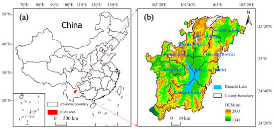
Figure 1. The map of the study area. (a) Location of the study area in China; (b) Elevation map of the study area.

2.2. Data Collection and Processing

NL data have been demonstrated to estimate socio-economic development dynamics [1]. Therefore, this study utilizes NL data to analyze the economic development of the Dianchi Lake region at the pixel scale. The NL data is sourced from a globally calibrated NPP-VIIRS-like dataset (Earth Observation Group, Colorado School of Mines, Golden, CO, USA), which includes cross-sensor data from DMSP-OLS and NPP-VIIRS, with a spatial resolution of 500 m. To standardize the analysis scale, the NL data from 2000 to 2022 was resampled to a 1000 m resolution using the nearest-neighbor method, and a spatiotemporal cube with 23 time dimensions was constructed as the foundation for this study.

This study aims to explore the factors influencing economic development in the Dianchi Lake region by selecting eight key variables based on the specific characteristics of the study area. These included human activity indicators (population density, road network density, GDP), topographic variables (DEM, slope, aspect), and climatic parameters (temperature and precipitation) (Table 1). It is important to note that, although GDP can also reflect economic development, it fundamentally differs from night-time light data derived from remote sensing. Thus, GDP is used in this study as an indicator of human activity. The data were standardized, and multicollinearity among variables was minimized using variance inflation factor (VIF) analysis to meet model requirements. Subsequently, the spatial association between the average values of these factors and the average NL from 2000–2020 was analyzed at a 1 km resolution. Additionally, 10 m resolution industrial land data were employed to assess the impact of industrial activity on economically active zones within the study area with high spatial precision.

Table 1. Data sources of influencing factors of economic development.

Category	Impact Factor	Abbreviation	Unit	Spatial Resolution	Time	Source	VIF
Human activity	Population Density	PD	$\mathrm{p}\mathrm{e}\mathrm{r}\mathrm{s}\mathrm{o}\mathrm{n}/\mathrm{k}{\mathrm{m}}^2$	1 km	2000–2022	Data from https://landscan.ornl.gov/ (before 24 December 2025) was used to calculate the annual average raster.	1.25
	Road Network Density	RD	$\mathrm{k}\mathrm{m}/\mathrm{k}{\mathrm{m}}^2$	1 km	2022	Calculated using ArcGIS (v10.8.1) based on Open Street Map (OSM) data.	1.64
	Gross Domestic Product	GDP	10,000 yuan	1 km	2000, 2005, 2010, 2015, 2020	Data from https://www.resdc.cn/ (before 24 December 2025) was used to calculate the average raster.	1.64
Topography	DEM	DEM	m	30 m	-	https://browser.dataspace.copernicus.eu/ (before 24 December 2025)	5.77
	Slope	Slope	°	30 m	-	Calculated using ArcGIS based on DEM.	1.34
	Aspect	Aspect	°	30 m	-		1.07
Climate	Temperature	TEM	°C	1 km	2000–2022	Calculating average raster [29,30].	6.50
	Precipitation	PRE	mm	1 km	2000–2022		2.71

2.3. Methods

2.3.1. Standard Deviation Ellipse

The standard deviation ellipse method estimates the spatial distribution of a dataset by computing its standard deviation and covariance, effectively capturing the spatial concentration, dispersion, and directional trends of the data [31]. The key components of the standard deviation ellipse include the mean center (centroid), major axis, minor axis, and azimuth angle [32]. This study applies multi-year standard deviation ellipse analysis to examine the spatial shifts in the economic development center of the area surrounding Dianchi Lake. The calculation formulas are as follows:

$${\overline{X}}_{\mathrm{w}}={\displaystyle \frac{{\sum }_{i=1}^n\hspace{0.17em}{w}_i{x}_i}{{\sum }_{i=1}^n\hspace{0.17em}{w}_i}},{\overline{Y}}_{\mathrm{w}}={\displaystyle \frac{{\sum }_{i=1}^n\hspace{0.17em}{w}_i{y}_i}{{\sum }_{i=1}^n\hspace{0.17em}{w}_i}}$$

(1)

$$\tan \theta ={\displaystyle \frac{{\sum }_{i=1}^n\hspace{0.17em}{w}_i^2{\tilde{x}}_i^2-{\sum }_{i=1}^n\hspace{0.17em}{w}_i^2{\tilde{y}}_i^2+\sqrt{({\sum }_{i=1}^n\hspace{0.17em}{w}_i^2{\tilde{x}}_i^2-{\sum }_{i=1}^n\hspace{0.17em}{w}_i^2{\tilde{x}}_i^2{)}^2-4{\sum }_{i=1}^n\hspace{0.17em}{w}_i^2{\tilde{x}}_i^2{\tilde{y}}_i^2}}{4{\sum }_{i=1}^n\hspace{0.17em}{w}_i^2{\tilde{x}}_i{\tilde{y}}_i}}$$

(2)

$${\delta }_x=\sqrt{{\displaystyle \frac{{\sum }_{i=1}^n\hspace{0.17em}(w_i{\tilde{x}}_i\mathrm{c}\mathrm{o}\mathrm{s}\theta -w_i{\tilde{y}}_i\mathrm{s}\mathrm{i}\mathrm{n}\theta {)}^2}{{\sum }_{i=1}^n\hspace{0.17em}{w}_i^2}}}$$

(3)

$${\delta }_y=\sqrt{{\displaystyle \frac{{\sum }_{i=1}^n\hspace{0.17em}(w_i{\tilde{x}}_i\mathrm{s}\mathrm{i}\mathrm{n}\theta -w_i{\tilde{y}}_i\mathrm{c}\mathrm{o}\mathrm{s}\theta {)}^2}{{\sum }_{i=1}^n\hspace{0.17em}{w}_i^2}}}$$

(4)

In the equations, ($x_i$, $y_i$) represent the spatial coordinates of the elements, and $w_i$ denotes the spatial weight. (${\overline{X}}_{\mathrm{w}}$, ${\overline{Y}}_{\mathrm{w}}$) corresponds to the weighted mean center of the elements. The parameter $\theta$ represents the azimuth angle of the standard deviation ellipse. Additionally, ${\tilde{x}}_i$ and ${\tilde{y}}_i$ denote the coordinate deviations of the elements from the mean center, while ${\delta }_x$ and ${\delta }_y$ represent the standard deviations along the x-axis and y-axis.

2.3.2. Defining the Space–Time Cube

The spatiotemporal cube, proposed by Hägerstrand in 1970, consists of spatial information, which represents the geometric shape and location of geographic objects, and temporal information, which denotes the time span of geographic entities or phenomena [33,34]. Due to its ability to depict temporal variations in three-dimensional geographic phenomena, the space–time cube model has been widely applied in various studies. In this research, annual average NL data from 2000 to 2022 were utilized to construct a pixel-level spatiotemporal cube, enabling a temporal perspective on the complex economic dynamics in the area surrounding Dianchi Lake (Figure 2).

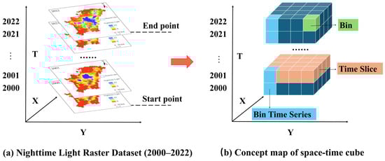
Figure 2. Diagram of constructing space–time cube.

2.3.3. Emerging Space–Time Hot Spot Analysis

Emerging space–time hot spot analysis can identify spatial and temporal trends in data, facilitating the detection of hot spot or cold spot locations. This method serves as an effective tool for understanding the implicit spatiotemporal relationships among spatial objects. The emerging hot spot analysis tool utilizes a spatiotemporal cube as input, computing the Getis-Ord Gi*. Subsequently, the Mann–Kendall trend test is employed to assess the temporal trends of these hot spots and cold spots, and each location within the study area is classified accordingly. In this study, to identify the hotspot patterns of economic development in the research area, a temporal dimension is incorporated into the Getis-Ord Gi* model. By applying a 1 km neighborhood distance and a one-year temporal step, the Gi* statistic for each column in the spatiotemporal cube is computed (Figure 3). The Getis-Ord Gi* calculation method is as follows:

$$G_i^{\ast }={\displaystyle \frac{{\sum }_{j=1}^n\hspace{0.17em}{\omega }_{i,j}{X}_j-\overline{X}{\sum }_{j=1}^n\hspace{0.17em}{\omega }_{i,j}}{\sqrt{\sqrt{\frac{n}{n-1{\sum }_{j=1}^n\hspace{0.17em}{\omega }_{i,j}^2}-\frac{1}{n-1{\left({\sum }_{j=1}^n\hspace{0.17em}{\omega }_{i,j}\right)}^2}}}}}$$

(5)

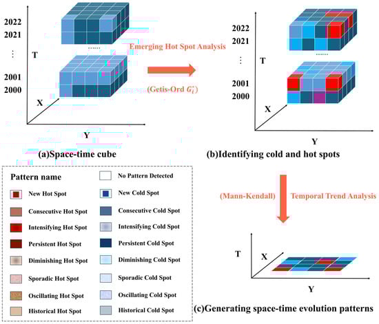
Figure 3. Process diagram of emerging space–time hot spot analysis. (a–c) represent the principles and calculation process of the emerging space–time hot spot analysis. “Pattern name” refers to all possible patterns for each pixel. The legend is the default setting from ArcGIS Pro (v3.6).

In this expression, $X_j$ represents the attribute value of element $j$, and ${\omega }_{i,j}$ denotes the weight between elements $i$ and $j$. If element $j$ lies within both the spatial proximity region and the temporal range of element $i$, then ${\omega }_{i,j}$ = 1; otherwise, ${\omega }_{i,j}$ = 0. $n$ denotes the total number of elements, and:

$$\overline{X}={\displaystyle \frac{1}{n}}\sum _{j=1}^n\hspace{0.17em}{X}_j$$

(6)

$$S=\sqrt{{\displaystyle \frac{1}{n}}\sum _{j=1}^n\hspace{0.17em}{X}_j^2-(\overline{X}{)}^2}$$

(7)

The results returned by the $G_i^{\ast }$ statistic consist of two values: (1) the Z-score at each location, where the $G_i^{\ast }$ value corresponds to the Z-score. The $G_i^{\ast }$ statistic helps identify significant hot spots (high-value clusters) and cold spots (low-value clusters). When the Z-score is positive, higher Z-scores indicate a stronger concentration of high values (hot spot); when the Z-score is negative, lower Z-scores suggest a tighter clustering of low values (cold spot) (Figure 3). (2) The p-value, which represents the reliability of the analysis results under different confidence levels. Table 2 presents the classification of cold spot and hot spot, with specific classifications referenced from the literature [35].

Table 2. Emerging spatiotemporal hot spot classification.

Z-Score	p-Value	Confidence	Pattern Name
<−2.58	<0.01	99%	Cold Spot
−2.58–−1.96	<0.05	95%	Cold Spot
−1.96–−1.65	<0.1	90%	Cold Spot
−1.65–1.65	-	-	Not significant
1.65–1.96	<0.1	90%	Hot Spot
1.96–2.58	<0.05	95%	Hot Spot
>2.58	<0.01	99%	Hot Spot

2.3.4. Local Outlier Analysis

To further investigate spatial correlation, the study employed Local Moran’s I to analyze local outliers in the NL spatial distribution and categorized the spatial correlations between different regions of the study area into four types: high-high clusters, low-low clusters, high-low clusters, and low-high clusters (Figure 4). The calculation formula for the Local Moran’s I is:

$$\begin{array}{c}{I}_i={\displaystyle \frac{\left(x_i-\overline{x}\right)}{S^2}}{\displaystyle \sum _j}\hspace{0.17em}{w}_{ij}\left(x_j-\overline{x}\right)\end{array}$$

(8)

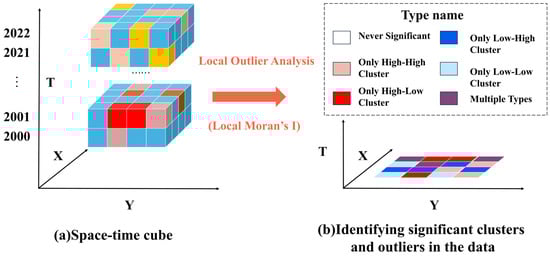
Figure 4. Process diagram of local outlier analysis. (a,b) represent the principles and calculation process of local outlier analysis. “Type name” refers to all possible types for each pixel. The legend is the default setting from ArcGIS Pro.

In this formula, $x_i$ represents the NL of region $i$, $\overline{x}$ is the mean NL of all regions, $S^2$ denotes the variance of NL, and the spatial weight matrix $w_{ij}$ was constructed using the nearest-neighbor method, which indicates the spatial relationship between regions $i$ and $j$.

The study determines the significance of the local Moran’s I using the $Z_i$.

$$Z_i={\displaystyle \frac{I_i-E\left(I_i\right)}{SD\left(I_i\right)}}$$

(9)

In this formula, $E\left(I_i\right)$ represents the expected NL value of region $i$, and $SD\left(I_i\right)$ denotes the standard deviation of the NL for region $i$.

2.3.5. Machine Learning Methods

Four machine learning models—Random Forest (RF), Support Vector Regression (SVR), Gradient Boosting Machine (GBM), and eXtreme Gradient Boosting (XGBoost)—were employed to analyze the influencing factors of economic development. All models were optimized using Bayesian optimization and validated through five-fold cross-validation to ensure model accuracy. (1) RF is an ensemble learning algorithm that constructs multiple decision trees using different subsets of the data and aggregates their outputs to produce the final prediction. It is robust to missing values and exhibits strong generalization capability [36]. (2) SVR, based on Support Vector Machine (SVM), seeks an optimal hyperplane in high-dimensional space that maximizes the margin between data points and the hyperplane to predict continuous variables. It offers excellent generalization ability and high predictive accuracy, with computational complexity independent of input dimensionality [37]. (3) GBM is an iterative ensemble model that applies the principle of gradient boosting by sequentially training multiple decision trees and combining their outputs in a weighted manner. It is capable of flexibly handling missing values, nonlinear relationships, and feature interactions [38]. (4) XGBoost, an enhanced version of GBM, incorporates regularization, parallel computation, and tree optimization techniques, enabling it to effectively handle sparse data. It is particularly suitable for datasets with high-dimensional features or missing values. Furthermore, by integrating both first- and second-order gradient information during optimization, it captures complex patterns more efficiently. These enhancements improve the model’s generalization ability and reduce overfitting, thereby enhancing predictive accuracy and robustness [39].

2.3.6. SHAP Algorithm

Despite their strong predictive performance, complex machine learning models are often regarded as “black boxes” due to the difficulty in interpreting their internal decision-making processes. SHAP (SHapley Additive exPlanations) is a powerful framework for interpreting the outputs of such models [40]. It offers both global and local explanations, facilitating a deeper understanding of model decisions while enhancing transparency and interpretability.

SHAP is based on the classical Shapley value from game theory, which attributes a model’s output to individual features by assigning them importance scores. Initially designed to fairly distribute gains among players in cooperative games, the Shapley value in machine learning quantifies each feature’s marginal contribution to a prediction. The formula for calculating Shapley values is as follows:

$${\varphi }_j=\sum _{S\subseteq N\setminus \left\{j\right\}}{\displaystyle \frac{\mid S\mid !\left(N-∣S∣-1\right)!}{N!}}\left(v\left(S\cup \left\{j\right\}\right)-v\left(S\right)\right)$$

(10)

In this expression, $N$ denotes the set of all features, $S$ represents a subset of features that excludes feature $j$,$v\left(S\right)$ indicates the model’s predicted value for the feature subset $S$, and $v\left(S\cup \left\{j\right\}\right)-v\left(S\right)$ represents the marginal contribution of feature $j$ to $S$. The term ${\displaystyle \frac{\mid S\mid !\left(N-∣S∣-1\right)!}{N!}}$ represents the associated weight.

3. Results and Analysis

3.1. Spatiotemporal Pattern Mining of Economic Development

3.1.1. The Trajectory of Economic Development

This study employs NL data and standard deviation ellipse analysis to examine the economic development direction in the Dianchi Lake region (Figure 5). The results indicate that from 2000 to 2022, the economic development centroid of the study area is located in the northern part of Dianchi Lake (Figure 5a), with the centroid trajectory shifting towards the northeast (Figure 5b) and southeast (Figure 5c). Specifically, economic development in the study area from 2000 to 2022 can be roughly divided into four stages: the centroid shifts eastward (2000–2004), southeast (2004–2012), northeast (2012–2020), and southwest (2020–2022).

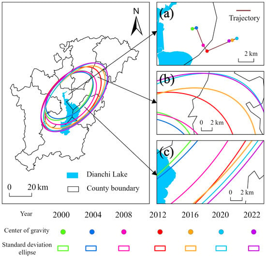
Figure 5. Spatial distribution map of the centroid and standard deviation ellipse of nighttime light from 2000 to 2022. (a): Centroid trajectory; (b,c): Standard deviation ellipses.

3.1.2. Spatiotemporal Distribution Characteristic

This study constructs a space–time cube model of economic development in the Dianchi Lake region using NL data (2000–2022) with a 1 km neighborhood range and a 1-year time step to examine regional economic disparities (Figure 6). The results show that areas near Dianchi Lake exhibit higher NL intensity, especially in the northern region, indicating greater economic development (Figure 6d). Furthermore, certain areas of Anning City (Figure 6a), Songming County (Figure 6b), and Jinning District (Figure 6c) also demonstrate significant economic development. Notably, the NL growth rate increased from 0.59 (2000–2012) to 0.72 (2013–2022), indicating a notable acceleration in economic development in the Dianchi Lake region (Figure 7).

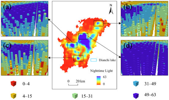
Figure 6. Spatial distribution map of nighttime light from 2000 to 2022. (a–d) represent the three-dimensional space-cube visualizations for different regions.

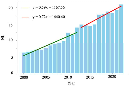
Figure 7. Temporal distribution map and linear fitting of the average nighttime light from 2000 to 2022.

3.1.3. Emerging Space–Time Hot Spot

This study conducts an emerging space–time hot spot analysis of the NL space–time cube, yielding the spatial distribution (Figure 8) and statistical results (Figure 9) of economic development hot spots in the Dianchi Lake region. The results show that 59.9% of the study area exhibits hot spots, primarily concentrated near Dianchi Lake, particularly in the northeastern region, indicating economic growth in these areas (Figure 8a,d). 40.1% of the region shows cold spots, mainly in the southern part of Anning City, the western part of Jinning District (Figure 8c), and the northern part of Panlong District (Figure 8b), indicating slower economic development in these areas. Notably, the hot spot pattern is predominantly continuous, suggesting that economic development has remained active in most areas of the study region. In contrast, the cold spot pattern is mainly historical and persistent, indicating consistently low levels of economic activity in these regions. This study highlights the imbalance in economic development across different areas of the Dianchi Lake region and reveals spatial and temporal heterogeneity.

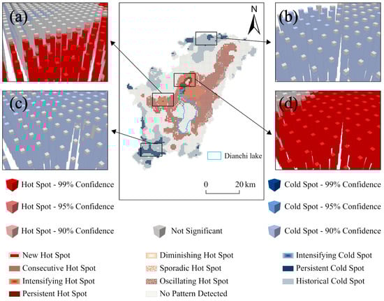
Figure 8. Spatial distribution map of emerging space–time hot spot of nighttime light from 2000 to 2022. (a–d) are the three-dimensional visualizations of emerging space–time hot spots for different regions.

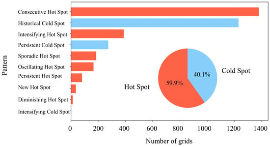
Figure 9. Grid statistical chart of emerging space–time hot spot.

3.1.4. Clustering of Local Outliers

This study employs the space–time cube of NL to examine the spatial clustering of economic development in the Dianchi Lake region using local outlier analysis (Figure 10). The results indicate that the spatial clustering types of economic development in the study area can be classified into three categories: high-high clustering, low-low clustering, and mixed types, accounting for 10.46%, 44.59%, and 44.95% of the study area, respectively. High-high clustering is predominantly observed in the northern part of Dianchi Lake (Figure 10a) and the northern part of Anning City (Figure 10b), indicating higher economic development levels and a distinct spatial aggregation effect. Low-low clustering is primarily found in the northern and southern areas of the study region, away from Dianchi Lake, indicating lower economic development levels and a similar spatial aggregation effect. The local outlier analysis results for economic development in areas surrounding Dianchi Lake reveal multiple categories, suggesting that spatial clustering in these areas has changed from 2000 to 2022.

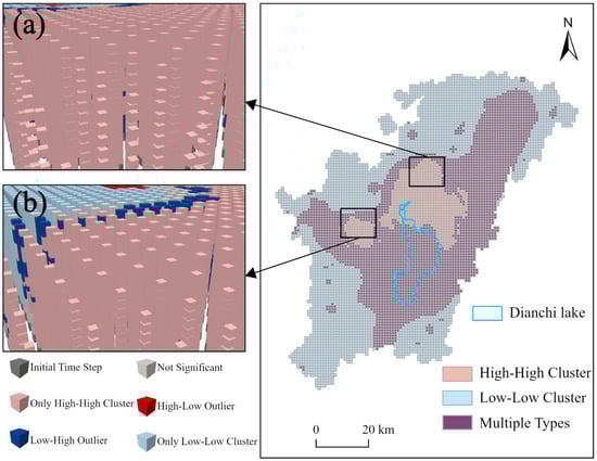
Figure 10. Spatial clustering map of local outliers for nighttime light from 2000 to 2022. (a,b) are the three-dimensional visualizations of local outliers for different regions.

3.2. Influencing Factors of Economic Development

3.2.1. Bivariate Spatial Relationship

This study employs a binary variable approach to analyze the spatial relationships between economic development and factors such as population density (PD), road network density (RD), GDP, DEM, slope, aspect, temperature (TEM), and precipitation (PRE) in the Dianchi Lake region (Figure 11). The results indicate that all eight factors exhibit significant spatial heterogeneity in relation to economic development, with the areas surrounding Dianchi Lake being the core of economic growth. Specifically, regions with high population density, road network density, and GDP—particularly in the northeastern area of Dianchi Lake—show higher levels of economic development. Conversely, areas with low population density, road network density, and GDP—mainly in the northern and southern parts of the study area—display lower economic development levels. Notably, in addition to the three common economic factors, areas near Dianchi Lake benefit from lower elevation, gentler slopes, and higher temperatures, which facilitate economic growth. In contrast, the northern and southern regions of the study area, characterized by higher elevation, steeper slopes, and lower temperatures, constrain economic development. This study underscores the influence of climate and topography on the economic development of the Dianchi Lake region.

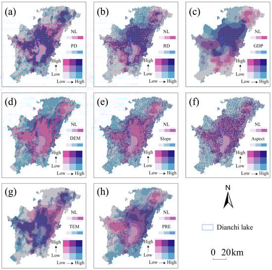
Figure 11. Bivariate spatial relationship map of nighttime light and various influencing factors. (a) Population density (PD), (b) Road network density (RD), (c) GDP, (d) DEM, (e) Slope, (f)Aspect, (g) Temperature (TEM), (h) Precipitation (PRE).

To further confirm that Dianchi Lake is the core of economic development in the study area, this study establishes eight buffer zones at 10 km intervals (Figure 12a). The results indicate that (Figure 12b), as the buffer zone distance increases, the NL values show a decreasing trend. Notably, when the buffer zone distance reaches 50 km and 60 km, NL values increase, which can be attributed to relatively better economic development in parts of Songming County in the northeastern region of Dianchi Lake, confirming that the economic development core has shifted northeast in recent years. Therefore, the study focuses on the northeastern region of Dianchi Lake to further explore the industrial impact on economic development (Figure 12c). The results show that (Figure 12d), NL values for industrial land in the built-up areas are significantly higher than those for non-industrial land in the built-up areas and non-built-up areas, suggesting that industry has a promoting effect on economic development.

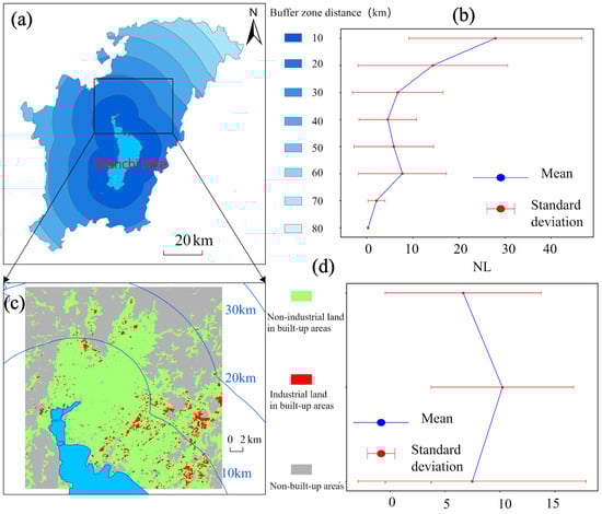
Figure 12. Buffer zone analysis based on Dianchi Lake and industrial impact analysis. (a) 10 km buffer zone distribution map; (c) Industrial distribution map in the northern part of Dianchi Lake; Nighttime light statistics at different buffer distances (b) and different industrial types (d).

3.2.2. Comparison of Machine Learning Models

To identify the optimal model for analyzing the influencing factors of economic development, this study compared the performance of four machine learning models on the training, testing, and full datasets (Table 3). To prevent overfitting, Bayesian optimization was employed to determine the optimal hyperparameters, and five-fold cross-validation was used during model training. For example, in the XGBoost model, parameters such as the number of trees, maximum depth, learning rate, and subsample ratio were optimized, and regularization was applied to further reduce overfitting. A similar optimization procedure was applied to each model to ensure optimal performance and stability. The four machine learning models were evaluated and compared. Consistent with previous studies, 70% of the full dataset was randomly allocated for training and the remaining 30% for testing. The results indicated that the XGBoost model achieved the highest R² and the lowest RMSE and MAE across all three datasets, demonstrating its superior predictive performance compared to the other models.

Table 3. Performance metrics of the four ML models on the training set, test set, and full dataset.

Model		XGBoost	RF	GBM	SVR
Training set	${\mathrm{R}}^2$	0.99	0.95	0.97	0.88
	RMSE	1.39	3.41	2.88	5.63
	MAE	0.95	2.44	2.02	3.37
Testing set	${\mathrm{R}}^2$	0.88	0.87	0.88	0.83
	RMSE	5.42	5.73	5.56	6.60
	MAE	3.66	3.96	3.81	4.38
Full dataset	${\mathrm{R}}^2$	0.96	0.93	0.94	0.86
	RMSE	3.19	4.24	3.88	5.94
	MAE	1.76	2.90	2.56	3.67

Furthermore, a Taylor diagram was used to provide a comprehensive comparison of the four machine learning models. The Taylor diagram concisely summarizes various aspects of model performance, including correlation, root mean square difference, and the matching of standard deviations. It is particularly suitable for evaluating complex models and has been widely used in Earth science research. In Figure 13, the red solid point on the x-axis represents the actual value with a correlation coefficient of one. The closer a predicted model point is to this reference, the better its performance. The results confirmed that the XGBoost model (with Python v3.11) had the best predictive performance. RF and GBM exhibited comparable results, both outperforming the SVR model, particularly on the training set.

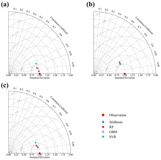
Figure 13. Taylor diagram illustrating the performance of the ML models on the training set (a), testing set (b), and full dataset (c). The ‘observation’ point indicates experimentally measured data, used for comparison with the models (XGBoost, RF, GBM, SVR).

3.2.3. Results of the ML Model

To quantitatively assess the importance of influencing factors on the economic development of the Dianchi Lake region, this study integrates the XGBoost and SHAP models, using SHAP values derived from the test set to represent variable importance (Figure 14). The importance contributions of human activity, climate, and topographic factors are 60.0%, 28.6%, and 11.4%, respectively (Figure 14a), indicating that human activity has the greatest impact on the region’s economic development, with GDP being the most significant individual factor. The summary plot results (Figure 14b) show that higher values of GDP, PD, TEM, PRE, and RD correspond to larger SHAP values, which are positively correlated with economic development, while DEM and Slope show the opposite trend.

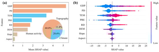
Figure 14. Feature importance (a) and summary plot (b) of economic development influencing factors based on the SHAP model.

To further analyze the nonlinear effects of each influencing factor on economic development in the Dianchi Lake region, this study quantified their impacts based on the variation in SHAP values with respect to feature values (Figure 15). Overall, GDP (c), PD (a), TEM (g), RD (b), and PRE (h) exhibited positive correlations with economic development, whereas DEM (d) and Slope (e) showed negative correlations, consistent with the results in Figure 15. Notably, the analysis highlighted the complex nonlinear relationships and threshold effects between influencing factors and economic development. For example, the influence of Aspect (f) on economic development fluctuated nonlinearly.

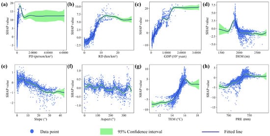
Figure 15. Dependency plots of economic impact factors: (a) Population Density (PD), (b) Road Network Density (RD), (c) GDP, (d) DEM, (e) Slope, (f) Aspect, (g) Temperature (TEM), and (h) Precipitation (PRE).

4. Discussion

4.1. The Space–Time Cube Illustrates Economic Development Dynamics

In the late 1960s, Hägerstrand proposed the space–time cube, widely regarded as the origin of time geography, though initially constrained by limited visualization capabilities [41]. Today, interactive and dynamic visualization tools such as ArcGIS Pro (v3.6) allow users to flexibly query and manipulate data within the space–time cube. This study employs the space–time cube to analyze the spatiotemporal dynamics of economic development in the Dianchi Lake region. Economic development hot spots are primarily concentrated around Dianchi Lake, particularly in the northeast, characterized by continuous hot spots with high-high clustering. In contrast, cold spots are predominantly located in the northern and southern parts of the study area, mostly as historical cold spots showing low-low clustering. These findings reflect marked spatial heterogeneity in economic development from 2000 to 2022, with sustained growth near the lake and slower development in the peripheral northern and southern regions. Previous research has confirmed that the Dianchi Basin is among the most socioeconomically dynamic regions in Yunnan Province [42]. The space–time cube not only visualizes the spatiotemporal distribution of geographic data but also enables temporal analysis, thereby improving the interpretability of complex spatiotemporal patterns. It serves as an effective tool in the field of geoscience.

4.2. The Application of Interpretable Machine Learning

Interpretable machine learning (IML) is widely recognized as an effective tool for exploring the driving mechanisms behind complex Earth systems. However, the rapid advancement of IML has often led to its application without sufficient attention to its inherent limitations, resulting in suboptimal research outcomes. Each machine learning model is based on specific assumptions and is suitable for particular data structures; therefore, it is crucial to align model selection with data characteristics to ensure reliable outcomes. Multicollinearity among variables can undermine model interpretability, especially in Earth sciences where variable coupling is prevalent. Without proper treatment, models may achieve good statistical fit while producing unreliable interpretations. This study emphasizes the importance of ensuring the validity of model interpretations in Earth science applications.

In this study, IML is used to analyze the factors influencing economic development in the Dianchi Lake region, including human activity, topography, and climate, thereby providing a methodological reference for the appropriate application of IML. Multicollinearity was mitigated through standardization and VIF analysis. Model performance was evaluated using R², RMSE, and MAE across training, testing, and full datasets to select the most suitable algorithm. Results indicate that human activity exerted the greatest influence on regional economic development. Among individual variables, GDP, population density, temperature, road network density and precipitation were positively associated with economic development, while DEM and slope exhibited negative correlations. Notably, IML revealed nonlinear relationships between predictors and economic development, offering valuable insights for policy optimization.

Despite its contributions, the study has several limitations: (1) Many intuitive economic indicators lack gridded data, which limits pixel-scale analysis of influencing factors; (2) The multi-source remote sensing data used in this study have varying spatial and temporal resolutions. (3) This study does not further investigate how interactions among human activity, climate, and topography jointly shape socioeconomic patterns in the Dianchi Lake Basin. Although the data were rescaled, potential multi-scale effects were not further explored. Future research should integrate higher-resolution socioeconomic microdata, land-use change data, and mobility-related datasets, and adopt multi-scale analytical frameworks to more comprehensively understand the drivers of regional economic development.

5. Conclusions

This study uses nighttime light (NL) data as a proxy for regional economic development to systematically analyze the spatiotemporal dynamics of economic development in the Dianchi Lake Basin from 2000 to 2022. An interpretable machine learning model was applied to examine the nonlinear effects of multiple influencing factors on economic development in the study area. The results show that economic development hotspots are mainly concentrated around Dianchi Lake, exhibiting persistent hotspot patterns with high–high spatial clustering, whereas cold spots are primarily distributed in the northern and southern parts of the region and are dominated by historical cold spots with low–low clustering. These findings provide an important theoretical basis for formulating more targeted and differentiated regional economic policies, such as promoting development in cold-spot areas and consolidating growth in hotspot regions. Unlike previous studies that have focused mainly on human activity factors (GDP, road network density, and population), this study further reveals that climatic factors (temperature and precipitation) are positively associated with economic development, while topographic factors (DEM and slope) exhibit negative associations, offering new perspectives on the driving mechanisms of economic development. Overall, this study underscores the importance of a long-term spatiotemporal perspective in analyzing regional economic development and confirms the applicability of interpretable machine learning within the frameworks of economic geography and regional development theory.

References

- Gu, Y.; Shao, Z.; Huang, X.; Cai, B. GDP Forecasting Model for China’s Provinces Using Nighttime Light Remote Sensing Data. Remote Sens. 2022, 14, 3671. [Google Scholar] [CrossRef]
- Cao, J.; Cao, X.; Tu, W.; Tan, X.; Wang, T.; Chen, G.; Zhang, X.; Li, Q. Nighttime light imagery or mobile phone footprints: Which better reflects urban socio-economics at the grid level? A case study in the Pearl River Delta, China. Comput. Environ. Urban Syst. 2025, 116, 102220. [Google Scholar] [CrossRef]
- Zhao, Z.; Tang, X.; Wang, C.; Cheng, G.; Ma, C.; Wang, H.; Sun, B. Analysis of the Spatial and Temporal Evolution of the GDP in Henan Province Based on Nighttime Light Data. Remote Sens. 2023, 15, 716. [Google Scholar] [CrossRef]
- Zhao, N.; Liu, Y.; Cao, G.; Samson, E.L.; Zhang, J. Forecasting China’s GDP at the pixel level using nighttime lights time series and population images. GISci. Remote Sens. 2017, 54, 407–425. [Google Scholar] [CrossRef]
- Liu, S.; Liu, W.; Zhou, Y.; Wang, S.; Wang, Z.; Wang, Z.; Wang, Y.; Wang, X.; Hao, L.; Wang, F. Analysis of Economic Vitality and Development Equilibrium of China’s Three Major Urban Agglomerations Based on Nighttime Light Data. Remote Sens. 2024, 16, 4571. [Google Scholar] [CrossRef]
- Jiang, W.; Liu, J.; Long, T.; Liu, M.; Pang, Z.; Luo, G.; Adam, E.; Ding, X.; Cui, S.; Wen, C.; et al. Preliminary analysis of factors affecting economic well-being based on SDGSAT-1 nighttime light remote sensing and household survey data. ISPRS Ann. Photogramm. Remote Sens. Spat. Inf. Sci. 2025, X-G-2025, 421–426. [Google Scholar] [CrossRef]
- Deng, Z.; Huang, J.; Ruan, C.; Li, J.; Gao, S.; Cai, Y. Volume-Based Space-Time Cube for Large-Scale Continuous Spatial Time Series. IEEE Trans. Vis. Comput. Graph. 2025, 31, 7019–7033. [Google Scholar] [CrossRef]
- Kristensson, P.O.; Dahlback, N.; Anundi, D.; Bjornstad, M.; Gillberg, H.; Haraldsson, J.; Martensson, I.; Nordvall, M.; Stahl, J. An Evaluation of Space Time Cube Representation of Spatiotemporal Patterns. IEEE Trans. Vis. Comput. Graph. 2009, 15, 696–702. [Google Scholar] [CrossRef]
- Huang, L.; Kong, F.; Lu, Q.; Huang, W.; Dong, Y.; Zhao, J.; Shang, J.; Zhang, H. Analysis of desert locust (Schistocerca gregaria) suitability in Yemen: An integrated evaluation based on MaxEnt and space–time cube approaches. Int. J. Digit. Earth 2024, 17, 2346266. [Google Scholar] [CrossRef]
- Mo, C.; Tan, D.; Mai, T.; Bei, C.; Qin, J.; Pang, W.; Zhang, Z. An analysis of spatiotemporal pattern for COIVD-19 in China based on space-time cube. J. Med. Virol. 2020, 92, 1587–1595. [Google Scholar] [CrossRef]
- Wu, P.; Meng, X.; Song, L. Identification and spatiotemporal evolution analysis of high-risk crash spots in urban roads at the microzone-level: Using the space-time cube method. J. Transp. Saf. Secur. 2022, 14, 1510–1530. [Google Scholar] [CrossRef]
- Fang, T.B.; Lu, Y. Constructing a Near Real-time Space-time Cube to Depict Urban Ambient Air Pollution Scenario. Trans. GIS 2011, 15, 635–649. [Google Scholar] [CrossRef]
- Luan, G.; Zhao, F.; Xia, J.; Huang, Z.; Feng, S.; Song, C.; Dong, P.; Zhou, X. Analysis of long-term spatio-temporal changes of plateau urban wetland reveals the response mechanisms of climate and human activities: A case study from Dianchi Lake Basin 1993–2020. Sci. Total Environ. 2024, 912, 169447. [Google Scholar] [CrossRef]
- Yang, F.; Shen, J.; Zhu, F.; Zhang, J. A cartographic generalization method for 3D visualization of trajectories in space–time cubes: Case study of epidemic spread. Int. J. Digit. Earth 2025, 18, 2474190. [Google Scholar] [CrossRef]
- Kim, M.; Lee, S. Identification of Emerging Roadkill Hotspots on Korean Expressways Using Space–Time Cubes. Int. J. Environ. Res. Public Health 2023, 20, 4896. [Google Scholar] [CrossRef] [PubMed]
- Liu, Y.; Hou, P.; Wang, P.; Zhu, J.; Zhai, J.; Chen, Y.; Wang, J.; Xie, L. Quantitative Analysis about the Spatial Heterogeneity of Water Conservation Services Function Using a Space–Time Cube Constructed Based on Ecosystem and Soil Types. Diversity 2024, 16, 638. [Google Scholar] [CrossRef]
- Del Castillo, M.F.P.; Fujimi, T.; Tatano, H. Spatiotemporal economic impact analysis of the Taal Volcano eruption using electricity consumption and nighttime light data. Geomat. Nat. Hazards Risk 2025, 16, 2445626. [Google Scholar] [CrossRef]
- Wang, C.; Qin, H.; Zhao, K.; Dong, P.; Yang, X.; Zhou, G.; Xi, X. Assessing the Impact of the Built-Up Environment on Nighttime Lights in China. Remote Sens. 2019, 11, 1712. [Google Scholar] [CrossRef]
- Beyer, R.C.M.; Franco-Bedoya, S.; Galdo, V. Examining the economic impact of COVID-19 in India through daily electricity consumption and nighttime light intensity. World Dev. 2021, 140, 105287. [Google Scholar] [CrossRef]
- Yang, Z.; Hong, Y.; Zhai, G.; Wang, S.; Zhao, M.; Liu, C.; Yu, X. Spatial Coupling of Population and Economic Densities and the Effect of Topography in Anhui Province, China, at a Grid Scale. Land 2023, 12, 2128. [Google Scholar] [CrossRef]
- Stuart, D.; Gunderson, R.; Petersen, B. Is a New Economic System Necessary to Address Climate Change? WIREs Clim. Change 2025, 16, e70003. [Google Scholar] [CrossRef]
- Musibau Ojo, A. Climate change and economy in nigeria: A quantitative approach. ACTA Econ. 2021, 19, 169–186. [Google Scholar] [CrossRef]
- Jiang, S.; Sweet, L.; Blougouras, G.; Brenning, A.; Li, W.; Reichstein, M.; Denzler, J.; Shangguan, W.; Yu, G.; Huang, F.; et al. How Interpretable Machine Learning Can Benefit Process Understanding in the Geosciences. Earths Future 2024, 12, e2024EF004540. [Google Scholar] [CrossRef]
- Molnar, C.; Casalicchio, G.; Bischl, B. Interpretable Machine Learning—A Brief History, State-of-the-Art and Challenges. In Joint European Conference on Machine Learning and Knowledge Discovery in Databases; Springer International Publishing: Cham, Switzerland, 2020. [Google Scholar]
- Liu, X.; Zheng, L.; Wang, Y. Revealing the roles of climate, urban form, and vegetation greening in shaping the land surface temperature of urban agglomerations in the Yangtze River Economic Belt of China. J. Environ. Manag. 2025, 377, 124602. [Google Scholar] [CrossRef] [PubMed]
- Zhang, J.; Ma, X.; Zhang, J.; Sun, D.; Zhou, X.; Mi, C.; Wen, H. Insights into geospatial heterogeneity of landslide susceptibility based on the SHAP-XGBoost model. J. Environ. Manag. 2023, 332, 117357. [Google Scholar] [CrossRef]
- Zhang, Z.; Li, J.; Hu, Z.; Zhang, W.; Ge, H.; Li, X. Impact of Land Use/Land Cover and Landscape Pattern on Water Quality in Dianchi Lake Basin, Southwest of China. Sustainability 2023, 15, 3145. [Google Scholar] [CrossRef]
- Zhang, Z.; Li, J.; Lu, Y.; Yang, L.; Hu, Z.; Li, C.; Yang, X. Temporal and spatial changes in land use and ecosystem service value based on SDGs’ reports: A case study of Dianchi Lake Basin, China. Environ. Sci. Pollut. Res. 2022, 30, 31421–31435. [Google Scholar] [CrossRef]
- Peng, S. 1-km Monthly Precipitation Dataset for China (1901–2023); National Tibetan Plateau Data Center: Beijing, China, 2020. [Google Scholar]
- Peng, S. 1-km Monthly Mean Temperature Dataset for China (1901–2023); National Tibetan Plateau Data Center: Beijing, China, 2024. [Google Scholar]
- Zhang, Y.; Jiang, P.; Cui, L.; Yang, Y.; Ma, Z.; Wang, Y.; Miao, D. Study on the spatial variation of China’s territorial ecological space based on the standard deviation ellipse. Front. Environ. Sci. 2022, 10, 982734. [Google Scholar] [CrossRef]
- Zhang, S.; Liu, J.; Chen, Y.; Pei, W.; Xuan, L.; Wang, Y. Investigating the Dynamic Change and Driving Force of Isolated Marsh Wetland in Sanjiang Plain, Northeast China. Land 2024, 13, 1969. [Google Scholar] [CrossRef]
- Hägerstraand, T. What about people in regional science? Pap. Reg. Sci. 1970, 24, 7–21. [Google Scholar] [CrossRef]
- Wang, S.; Liu, M.; Li, Y.; Wu, L.; Zhou, B.; Tian, L. Spatiotemporal Cube Model Based on Stress Features for Identification of Heavy Metal Stress in Rice. IEEE Trans. Geosci. Remote Sens. 2024, 62, 4401313. [Google Scholar] [CrossRef]
- Feng, Y.; Huang, D.; Hong, X.; Wang, H.; Loughney, S.; Wang, J. Spatial-Temporal Evolution of Maritime Accident Hot Spots in the East China Sea: A Space-Time Cube Representation. J. Mar. Sci. Eng. 2025, 13, 233. [Google Scholar] [CrossRef]
- Xu, Q.; Yang, F.; Hu, S.; He, X.; Hong, Y. Tree Height–Diameter Model of Natural Coniferous and Broad-Leaved Mixed Forests Based on Random Forest Method and Nonlinear Mixed-Effects Method in Jilin Province, China. Forests 2024, 15, 1922. [Google Scholar] [CrossRef]
- Awad, M.; Khanna, R. Support Vector Regression. In Efficient Learning Machines; Apress: Berkeley, CA, USA, 2015; pp. 67–80. [Google Scholar]
- Friedman, J.H. Greedy function approximation: A gradient boosting machine. Ann. Stat. 2001, 29, 1189–1232. [Google Scholar] [CrossRef]
- Ptr, A.F.L.; Siregar, M.M.; Daniel, I. Analysis of Gradient Boosting, XGBoost, and CatBoost on Mobile Phone Classification. J. Comput. Netw. Archit. High Perform. Comput. 2024, 6, 661–670. [Google Scholar] [CrossRef]
- Lundberg, S.M.; Lee, S.-I. A Unified Approach to Interpreting Model Predictions. In Advances in Neural Information Processing Systems 30; Guyon, I., Luxburg, U.V., Bengio, S., Wallach, H., Fergus, R., Vishwanathan, S., Garnett, R., Eds.; Curran Associates Inc.: Red Hook, NY, USA, 2017; pp. 4765–4774. [Google Scholar]
- Kraak, M.J. The space-time cube revisited from a geovisualization perspective. In Proceedings of the 21st International Cartographic Conference, Durban, South Africa, 10–16 August 2003; International Cartographic Association: Wellington, New Zealand, 2003; pp. 1988–1996. [Google Scholar]
- Dawei, Z. Impacts of 20-year socio-economic development on aquatic environment of Lake Dianchi Basin. J. Lake Sci. 2012, 24, 875–882. [Google Scholar] [CrossRef]
Disclaimer/Publisher’s Note: The statements, opinions and data contained in all publications are solely those of the individual author(s) and contributor(s) and not of MDPI and/or the editor(s). MDPI and/or the editor(s) disclaim responsibility for any injury to people or property resulting from any ideas, methods, instructions or products referred to in the content. |
© 2025 by the authors. Licensee MDPI, Basel, Switzerland. This article is an open access article distributed under the terms and conditions of the Creative Commons Attribution (CC BY) license.