Optimised DNN-Based Agricultural Land Cover Mapping Using Sentinel-2 and Landsat-8 with Google Earth Engine

Abstract

Agriculture is the backbone of Punjab’s economy, and with much of India’s population dependent on agriculture, the requirement for accurate and timely monitoring of land has become even more crucial. Blending remote sensing with state-of-the-art machine learning algorithms enables the detailed classification of agricultural lands through thematic mapping, which is critical for crop monitoring, land management, and sustainable development. Here, a Hyper-tuned Deep Neural Network (Hy-DNN) model was created and used for land use and land cover (LULC) classification into four classes: agricultural land, vegetation, water bodies, and built-up areas. The technique made use of multispectral data from Sentinel-2 and Landsat-8, processed on the Google Earth Engine (GEE) platform. To measure classification performance, Hy-DNN was contrasted with traditional classifiers—Convolutional Neural Network (CNN), Random Forest (RF), Classification and Regression Tree (CART), Minimum Distance Classifier (MDC), and Naive Bayes (NB)—using performance metrics including producer’s and consumer’s accuracy, Kappa coefficient, and overall accuracy. Hy-DNN performed the best, with overall accuracy being 97.60% using Sentinel-2 and 91.10% using Landsat-8, outperforming all base models. These results further highlight the superiority of the optimised Hy-DNN in agricultural land mapping and its potential use in crop health monitoring, disease diagnosis, and strategic agricultural planning.

1. Introduction

Remote sensing plays a major role in agricultural research activities. Satellite imagery collects data for crop monitoring, soil type, agriculture practices, field management, and environmental monitoring. Various satellite datasets, including Sentinel-1/2, Landsat series, Moderate Resolution Imaging Spectroradiometer (MODIS), and Soil Moisture Active Passive (SMAP), have been utilised in agricultural applications [1,2]. These satellite sensors have varying technical properties, including spectral bands, spatial resolution, temporal resolution, swath width, and sensor type. After selecting a satellite dataset, pre-processing is required to enhance image quality, including noise reduction, geometric and cloud correction and atmospheric correction, while spatial and temporal coherence must also be confirmed [3]. Land use and land cover (LULC) classifications play a critical role in planning and promoting sustainable development, particularly in mountainous regions [4]. Previous studies have utilised various classifiers for urban and agricultural applications, demonstrating the strengths of machine learning in enhancing accuracy. One such study focused on Tehsil Karna Prayag in Uttarakhand, employing multispectral Sentinel-2 imagery, along with machine learning algorithms like Extreme Gradient Boosting (XGBoost) and K-nearest neighbour (KNN), to classify seven land cover categories. This paper used limited spectral bands (RGB and NIR) and excluded the SWIR and red-edge band, which can improve the classification of vegetation [5]. The results highlighted forests and fallow lands as the dominant classes, covering nearly 60% and 15% of the area, respectively, underscoring the importance of LULC analysis in effective land management.

In another case, the Barrackpore subdivision of West Bengal, India, served as a testbed for analysing urban expansion using Landsat data from 2005 and 2020. This research utilised parametric classifiers such as maximum likelihood classification (MLC) and Minimum Distance Classifier (MDC), with these two algorithms yielding the highest overall classification accuracy for their respective years. This study had limited ability to detect fine-scale land cover changes in urban and mixed-use areas because of the low (30 m) resolution image of Landsat-5 and Landsat-8 [6,7]. A similar effort in the Baghdad region utilised Landsat imagery to monitor changes post-2015, including urban growth and slum expansion resulting from a housing shortage. Change detection techniques and classification were implemented using ENVI (Environment for Visualising Images) software and custom Visual Basic routines to assess the transformation in vegetation and built-up areas. This study implemented two classification methods with datasets of moderate spatial resolution of 30 m but lacks quantitative accuracy assessments like a confusion matrix, OA, and KC [8]. Another study emphasised the relevance of LULC classification for urban development in developing countries, leveraging classification and regression trees (CART) within the Google Earth Engine (GEE) platform. The method demonstrated a strong classification accuracy of 92.9%, suggesting its potential for future applications in urbanisation and resource planning but showed limited class-specific accuracy, with 14% for bare land, and had a low spatial resolution for the LC map at 5 km [9].

In Brazil’s environmentally sensitive Quadrilátero Ferrífero region, machine learning algorithms, including Random Forest (RF), Support Vector Machine (SVM), and KNN, were tested for LULC classification. The study used remote sensing data for image segmentation to achieve F1-scores ranging from 0.89290 to 0.92994, indicating robust classification performance [10]. For the Babylon Governorate, researchers applied SVM, Minimum Distance (MD), and MLC using Landsat imagery to classify four land categories: built-up, water, barren, and agricultural land. Among these, SVM provided the highest overall accuracy of 86.88%, outperforming the other methods, but used a moderate spatial resolution of 30 m and limited training data samples of 160 [11]. In Ranya city, Sentinel-2 and Landsat 8 datasets were used to assess various classification models, including SVM and RF. Sentinel-2 data with RF delivered an overall accuracy of 83%, while SVM achieved a 92% accuracy in extracting building footprints, reinforcing the value of Sentinel-2 for accurate LULC mapping [12].

Machine learning and AI also play significant roles in agricultural LULC applications. Techniques like neural networks, SVM, and RF have been employed to predict crop yields based on satellite reflectance data. A deep learning comparison using Sentinel-1 and Landsat-8 in Ukraine assessed Convolutional Neural Network (CNN) and RF models for crop and land cover classification [13]. Additionally, Landsat-8 and multi-temporal imagery, alongside parameters such as weather, temperature, wind, and soil type, have been used in combination with algorithms like SVM and Artificial Neural Networks (ANN) to monitor agricultural land changes and crop growth stages [14]. A 160 km study area in Australia was analyzed using MLC for LULC classification. Initially, the results showed low accuracy, but improvements were achieved through a post-classification framework integrating digital elevation model (DEM), normalized difference vegetation index (NDVI), and post-classification correction (PCC), enhancing the classification reliability and demonstrating that implementation of MLC classifiers with other classification methods can achieve better accuracy [15].

Along with traditional classification methods and off-the-shelf satellite datasets, the last few years have seen the introduction of benchmark platforms and large datasets, which have radically improved the art of land cover and agriculture monitoring. DeepGlobe offers a world benchmark on land cover classification from high-resolution satellite images and deep learning frameworks, with support for semantic segmentation tasks and standardised evaluation protocols. Sen2Agri, created by the European Space Agency (ESA), provides an automatic processing chain for creating crop type maps and vegetation indices from time series of Sentinel-2 and Landsat-8 data and is thus very useful for national and regional agricultural monitoring. BigEarthNet, another influential output, is a large-scale, multi-label dataset constructed from Sentinel-2 imagery and allows robust training of deep learning models for various land cover classes over Europe. Although their utility and use in other remote sensing applications have been attested, these techniques were not used in the earlier studies discussed above. Incorporation of such benchmark systems situates this work at the forefront of LULC studies. Integration with these techniques increases the scientific rigor, reproducibility and relevance of classification frameworks such as Hy-DNN, making them more applicable across other geospatial environments.

The present study uses the GEE [16,17,18] platform to implement research work and develop a Hyper-tuned Deep Neural Network (Hy-DNN) for different i.e., multispectral datasets, Sentinel-2 and Landsat-8. The objectives are as follows: (a) to perform pre-processing of multispectral satellite datasets Sentinel-2 and Landsat-8 (OLI); (b) to design the framework for Hy-DNN and implement classification using the designed Hy-DNN and different classifiers, i.e., RF, MDC, CART, and NB, CNN i.e.; and (c) to compare and validate the designed Hy-DNN’s performance, and compute the accuracy assessment of each classifier with multispectral datasets. This study was conducted in the state of Punjab, India.

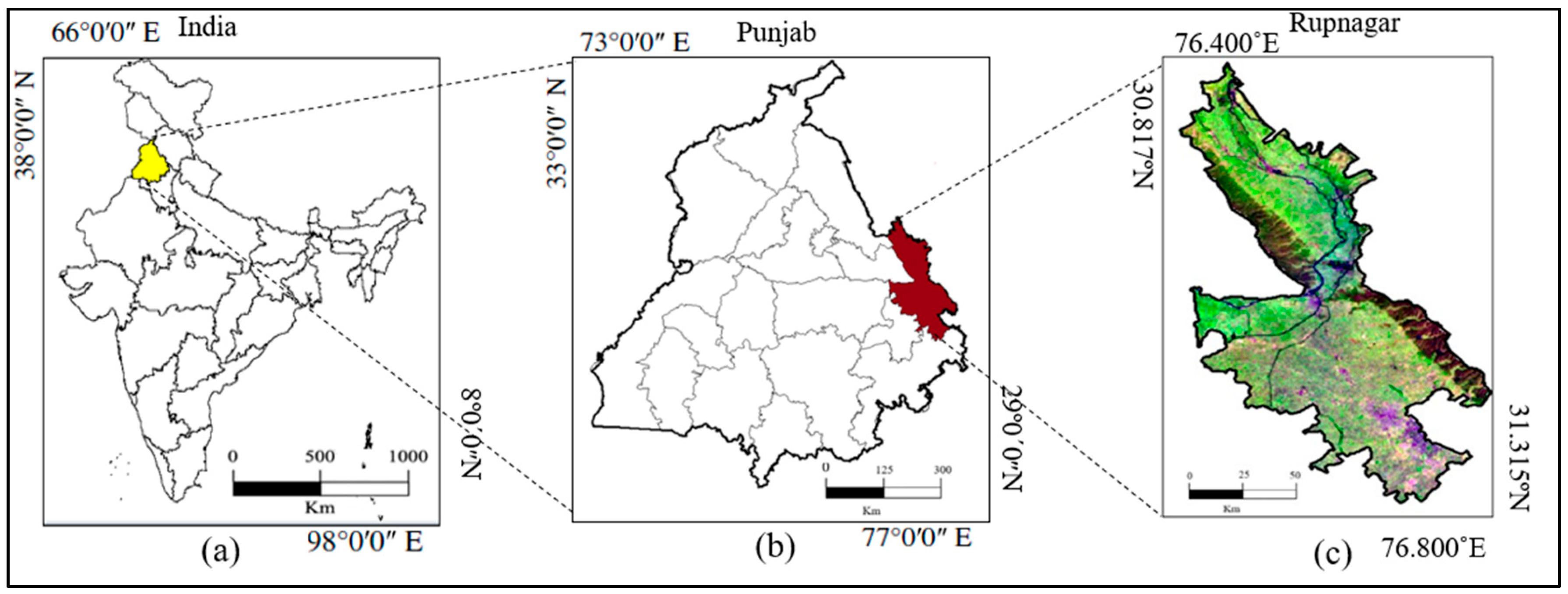
2. Study Site and Satellite Dataset

Rupnagar, a district in Punjab, India, is selected as the study area for this research. Geographically, it lies between latitudes 31.315° N in the northwest and 30.817° N in the southeast and extends from longitudes 76.400° E to 76.800° E, spanning approximately 1400 square kilometers, as shown in Figure 1. The study focuses on four land use categories: vegetation land, agricultural land, waterbodies, and built-up land. Agriculture plays a significant role in the region, with cropland forming a major component of the agricultural landscape. This makes Rupnagar an essential contributor to Punjab’s agrarian economy. The study area encompasses a diverse range of land use patterns, highlighting the importance of agriculture in sustaining livelihoods and supporting food security in India.

Satellite Dataset

In this article, the two satellite datasets, Landsat-8 and Sentinel-2, have been considered for agriculture analysis, as outlined in

Table 1. Technical specifications of Landsat-8 and Sentinel-2 satellite datasets.

Factors	Landsat-8	Sentinel-2
Sensor Types	OLI-2 (Operational Land Imager-2, TIRS-I (Thermal Infrared Sensor)	Multispectral imager (MSI)
Spectral Bands	It works on 11 spectral bands: OLI-2 works on multispectral bands 1–9 (0.43–1.38 µm), TIRS works on panchromatic band 10 (10.6 + 0–11–19 µm), and Band 11 (11.5–12.51 µm).	It uses 13 Spectral bands from visible to the infrared (VIS/NIR)
Spatial Resolution	Bands 1–7 and 9: 30 m, Band 8: 15 m, Band 10–11: 100 m	10 m (VIS/NIR bands), 20 m (red-edge and SWIR bands, and 60 m (atmospheric correction bands)
Temporal Resolution	16 days	5 days
Swath Width	185 km	290 km
Orbit	Sun-synchronous, near-polar orbit	Sun-synchronous, near-polar orbit
Data Format	GeoTIFF	JPEG 2000, XML with metadata
Operational	11 February 2013	23 January 2015

. Landsat-8 works on a total of 11 spectral bands. Bands 1–7 and 9 work on 30 m, band 8 works from 15 m, and bands 10–11 work on 100 m [19]. The Sentinel-2 dataset provided by the European Space Agency (ESA) used a spatial resolution of 10 m (VIS/NIR bands), 20 m (red-edge and SWIR bands), and 60 m (atmospheric correction bands) [20]. It works with a multispectral imager sensor, with 13 spectral bands, 290 km swath width, and 5 days temporal resolution [21].

3. Materials and Methods

This proposed framework consists of three main sections as shown in Figure 2a: satellite datasets pre-processing, Hy-DNN design and model training, application of classification using various algorithms, and accuracy assessment.

3.1. Pre-Processing

Pre-processing is a critical first step after data selection and addresses various errors. These errors can arise from factors such as the sun’s position, shifting atmospheric conditions, and inaccuracies in satellite sensors. Sentinel-2 and Landsat-8 data processing involves several corrections, including radiometric and atmospheric adjustments. These corrections are necessary to compensate for illumination differences caused by sensor calibration and atmospheric effects [22]. Firstly, the area of interest (AOI) is selected and we zoom in to the study site. After that, we apply date filters to choose the data, perform cloud masking, and then apply band median stacking filtering on the selected data from the multispectral Sentinel-2 [15]. Data are pre-processed using the GEE platform, which pre-processes the Sentinel-2 [23] and Landsat-8 datasets using Sen2core (Sentinel-2 ground segment processor) and Land Surface Reflectance Code (LaSRC) algorithms, respectively. These algorithms pre-processes the radiometric corrections for the satellite datasets [24].

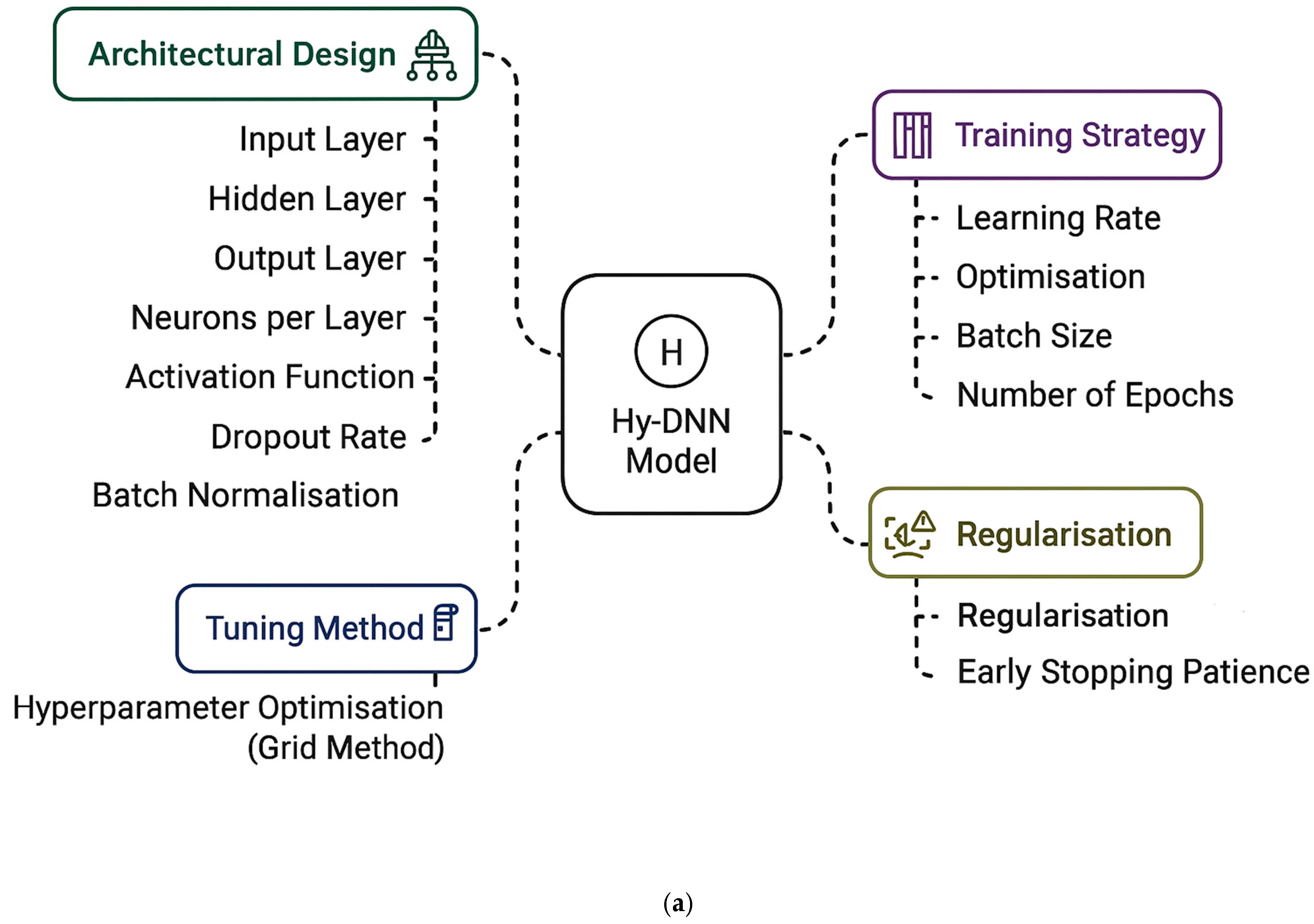
3.2. Hyper-Tuned Deep Neural Network (Hy-DNN)

The Hy-DNN framework provides a comprehensive workflow for land cover classification using satellite imagery and a deep learning-based approach, as illustrated in Figure 2b. The process initiates with satellite data collection, which serves as the primary source for land surface analysis. The first step involves selecting the AOI and filtering the satellite data to remove irrelevant or low-quality scenes. It uses U-Net architecture. Pre-processing techniques are applied to enhance the data by correcting radiometric and atmospheric distortions [1]. The refined satellite dataset is then processed through scripts executed on the GEE [25], a platform to extract and download selected spectral bands necessary for classification tasks.

Next, mosaicking is implemented on the satellite images using ERDAS (Earth Resources Data Analysis System) (2015) [26] software to produce a seamless and spatially continuous dataset. ERDAS offers comprehensive control over all parameters like feathering, histogram matching, and blending. This level of detailed customization allows for precise adjustment of the mosaic output, which is not achievable with the automated processes available in Google Earth Engine (GEE). Field observation data are simultaneously collected to serve as ground truth, aiding in the training and validation of the classification model. The satellite dataset is then sampled in the ENVI software (V5.6) with Deep Learning Module (V1.4), where 80% of the data are used for training and 20% for testing [27]. Features are extracted from the sampled data using a Hy-DNN model. This Hy-DNN model, consisting of input, hidden, and output layers, is trained using optimised hyperparameters to enhance classification accuracy. The model employed in this study was configured with the following specific hyper-tuned parameters to optimise classification performance.

The superior performance of the proposed Hyper-tuned Deep Neural Network (Hy-DNN) used U-net [28] architecture, and its performance over traditional classifiers such as Random Forest (RF), Classification and Regression Tree (CART), Minimum Distance Classifier (MDC), and Naive Bayes (NB) can be attributed to both its architectural depth and optimised learning strategy. Yet, in contrast to shallow models like RF and CART that depend on decision trees constructed from a few feature splits, or statistical models like NB and MDC based on independence or Euclidean separability, Hy-DNN has a multi-layer structure with the ability to model complicated non-linear relationships inherent in multispectral satellite data. The deep structure of the model supports hierarchical feature learning in which early layers learn low-level spectral data, and subsequent layers increasingly learn high-level spatial and contextual features that are pertinent in differentiating agricultural land cover classes.

In addition, the Hy-DNN architecture includes a hyperparameter optimisation procedure that utilises grid search for optimal tuning of key parameters, including learning rate, momentum, layer neurons, activation functions, and dropout levels. This guarantees that the network attains a balance between learning and generalisation capacity, reducing both underfitting and overfitting. Methods such as dropout regularisation and early stopping also continue to boost the model’s robustness, especially in dealing with imbalanced class distributions and changing spectral signatures of different land cover classes. Conversely, conventional machine learning algorithms frequently take advantage of manual feature design and are class-overlap and noise-sensitive in high-dimensional spaces. For instance, MDC assumes a uniform variance within classes and linear separability across classes, which is seldom valid in diverse environments. Naive Bayes is also inefficient when there are correlated features, as is frequently the case in remote sensing imagery. RF and CART, though very effective in most situations, are restricted by their ensemble depth and inability to acquire spatial relationships unless specially engineered.

The hyperparameter tuning process employed a grid search approach to evaluate various combinations of parameters, as shown in Figure 3a, including learning rate (ranging from 0.1 to 0.5), momentum (0.5 to 0.9), number of neurons in the hidden layer (6 to 20), and different activation functions. Each configuration was trained for up to 1000 epochs, with performance assessed through cross-validation and a 20% holdout test set. The optimal configuration was selected based on the best balance between training accuracy and generalisation error. To prevent overfitting, early stopping was applied using a convergence criterion of 0.1 for the root mean square error (RMSE) [29]. Additionally, dropout rates between 0.2 and 0.5 were manually adjusted to determine the most effective regularisation level for each dataset. This comprehensive tuning strategy ensured the final Hy-DNN model was well-suited to the spectral and spatial complexities of Sentinel-2 and Landsat-8 satellite imagery.

Once trained, the model is used to classify the satellite image, and the output is uploaded back to the GEE [30,31] platform. The testing samples are then used to validate the model’s performance. The final step involves conducting an accuracy assessment, typically through the generation of a confusion matrix and accuracy assessment parameters, including the F1-score [32], producer’s accuracy (PA), consumer’s accuracy (CA), Kappa coefficient (KC) [33], and overall accuracy (OA), to evaluate how well the model distinguishes between different land cover classes. This integrated approach leverages satellite remote sensing, field data, machine learning, and cloud-based platforms, ensuring accurate and scalable land cover classification. It benefits environmental monitoring, resource management, and land use planning.

3.3. Cross-Referencing with Other Machine Learning Classification Algorithms

In the current research paper, the machine learning classification algorithms (a) RF, (b) CART, (c) MDC, (4) NB, and (5) CNN [34] are also used for the classification of multispectral datasets, and their workflow is also discussed in Figure 3b. The testing is also performed with these classifiers. All the results are compared with the designed Hy-DNN model results. The best results are achieved with the hyper-tuned DNN compared to the RF, CART and MDC, and NB methods, after pre-processing of the datasets.

3.3.1. Random Forest (RF)

RF is used for classification and regression datasets [35]. It creates random DTs by using bootstrap sampling. Instead of selecting all the features, only a random subset of features is used for each DT [36]. An aggregation layer is added, which produces the average of all trees to produce the results.

The output layer is added and produces $(1+x)^n=1+nx/1!+\left(n\right(n-1) x^2)/2!$ The final result is obtained with the following steps:

Step 1: In the initial stage, select multiple training samples for different classes based on field observation and spectral signatures.

Step 2: Select satellite bands [37] for classification.

Step 3. After selecting the sample file, use the spectral signature to train the algorithm.

Step 4. Divide the dataset into two groups: 80% for training, and 20% for testing.

Step 5. Train the base model and implement a grid to find the best parameters for tuning.

Step 6. Train a random forest and implement bootstrap sampling to produce DTs, and then assign the class to majority voting.

Step 7. Obtain the final classification prediction in classification using majority voting:

$$\mathrm{ŷ}=\arg c max\sum _{t=1}^N\left(yt=\mathrm{c}\right)$$

(1)

where $N$ is the number of trees, $yt$ is the class prediction by the tree $t$, and the final class $\mathrm{ŷ}$ is the one that obtains the most votes.

3.3.2. CART

CART is a classification and regression tree prediction model used for classification and regression tasks. It describes how the target variable’s value can be predicted based on other values. [38]. It follows these steps.

Step 1: In the initial stage, select multiple training samples for different classes based on field observation and spectral signatures.

Step 2: Select satellite bands for classification.

Step 3. After selecting the sample file, the use spectral signature to train the algorithm.

Step 4. Divide the dataset into two groups: 80% for training, and 20% for testing.

Step 5. Split the node into the minimum splitting [39] sections using Gini indexing.

Step 6. Start recursive tree building and assign the class to the leaf node.

Step 7. Finally, generate the classified map.

$$Gini(s)=1-\sum _{i=0}^c{(pi)}^2$$

(2)

where $S$ is the dataset at a particular node, $c$is the number of classes, and pi is the probability of a sample belonging to class $i$.

3.3.3. Minimum Distance Classifier

The MDC is utilised in scenarios that demand efficient classification. It considers varying centroid and variance values to categorise pixels into distinct classes [38]. Widely applied in remote sensing and machine learning, MDC assigns an unknown sample to the nearest class by measuring the distance in feature space. It includes the following steps:

Step 1: In the initial stage, select multiple training samples for different classes based on field observation and spectral signatures.

Step 2: Select satellite bands for classification.

Step 3. After the sample file, use the spectral signature to train the algorithm.

Step 4. Divide the dataset into two groups: 80% for training, and 20% for testing.

Step 5. Calculate the class centroid and select the distance matrix.

Step 6. Compute the distance and assign the class based on the distance.

Step 7. Finally, generate the classified map based on distance. The following formula assigns the class centroid. It finds the distance between each pixel and class centroids, and pixel x is classified into class k with the minimum distance [40].

$$\mu k={\displaystyle \frac{1}{Nk}}\sum _{i=0}^{Nk}xi$$

(3)

where $Nk$ is the number of training samples in class k, and $xi$ is the feature vector of the sample $i.$

3.3.4. Naive Bayes

The classifier is a probabilistic classifier based on a machine learning algorithm, and it works as Bayes’ Theorem. It is used for classification tasks where all the features are independently given under the class label [41]. It is a fast and efficient algorithm for larger datasets. It can handle multiclass problems very easily.

Step 1: In the initial stage, select multiple training samples for different classes based on field observation and spectral signatures.

Step 2: Select satellite bands for classification according to classes.

Step 3. After the sample file, use the spectral signature to train the algorithm.

Step 4. Divide the dataset into two groups: 80% for training, and 20% for testing.

Step 5. Estimate the probability distribution parameters and calculate log-likelihoods.

Step 6. Calculate log-likelihoods and assign the class based on Bayes’ theorem [42].

Step 7. Finally, generate the classified map based on log values according to the formula where C is the class and X is the feature vector.

$$P\left(Ck\right|X)={\displaystyle \frac{\mathrm{P}\left(\mathrm{X}|\mathrm{C}\mathrm{k}\right)\mathrm{P}\left(\mathrm{C}\mathrm{k}\right)}{\mathrm{P}\left(\mathrm{X}\right)}}$$

(4)

3.3.5. Convolution Neural Network

A CNN (Convolutional Neural Network) is a deep learning model used primarily for image processing, classification, and object detection. Here are the step-by-step stages of how a CNN works:

Step 1. Multispectral data input layer: The default 3-channel ResNet [43] input is adapted to take in multiple spectral bands (for example, 4 channels: RGB + NIR) specific to satellite imagery.

Step 2. Residual learning enhances gradient flow: ResNet employs shortcut connections to make it possible to train deeper networks without vanishing gradients and thus provide improved feature representation.

Step 3. Feature extraction via convolutional layers: The network learns spatial patterns from a sequence of convolutional, ReLU, and pooling layers applied to all image patches.

Step 4. Classification via fully connected layers: The last FC layer is adjusted to have the same number of land cover classes, and the output is passed through softmax to obtain class probabilities.

Step 5. Training setup process: Training/testing splits, loss function (cross-entropy), and an optimisation strategy (e.g., Adam) are performed.

Step 6. Evaluation using standard metrics: CNN performance is measured in terms of overall accuracy (OA), Kappa coefficient, and per-class accuracy.

Step 7. Visualisation of results in the form of a thematic map: The output from CNN classification is represented as a thematic map consisting of 4 classes.

3.4. Accuracy Assessment

An accuracy assessment was conducted to validate the results of the classification algorithms, which is a critical step in the evaluation process. A stratified sampling method was employed to select representative samples for each land cover class (agriculture, vegetation, built-up, and waterbody) across the image, based on ground truth data. Several key parameters were considered in the assessment, including PA, CA, KC, and OA, for both the Sentinel-2 and Landsat-8 datasets [37]. PA = 100% − OE (omission error), and OA represents the ratio of correctly classified pixels to the total number of reference pixels for each class. CA = 100% − CE (commission error) also reflects the ratio of correctly classified pixels to the total reference pixels [44]. The KC measures the agreement between the classified map and reference data, accounting for chance agreement. It can be calculated as follows:

$$KC={\displaystyle \frac{Po-pe}{1-\mathrm{p}\mathrm{e}}}$$

(5)

where $KC$ is the Kappa coefficient, $po$ is the observed agreement, and $pe$ is the expected agreement. OA is calculated as the ratio of correctly classified pixels to the total number of pixels. It can be calculated as follows:

$$\mathrm{O}\mathrm{A}={\displaystyle \frac{\mathrm{c}\mathrm{o}\mathrm{r}\mathrm{r}\mathrm{e}\mathrm{c}\mathrm{t}\mathrm{l}\mathrm{y} \mathrm{c}\mathrm{l}\mathrm{a}\mathrm{s}\mathrm{s}\mathrm{i}\mathrm{f}\mathrm{i}\mathrm{e}\mathrm{d} \mathrm{s}\mathrm{a}\mathrm{m}\mathrm{p}\mathrm{l}\mathrm{e}\mathrm{s}}{\mathrm{t}\mathrm{o}\mathrm{t}\mathrm{a}\mathrm{l} \mathrm{n}\mathrm{u}\mathrm{m}\mathrm{b}\mathrm{e}\mathrm{r} \mathrm{o}\mathrm{f} \mathrm{s}\mathrm{a}\mathrm{m}\mathrm{p}\mathrm{l}\mathrm{e}\mathrm{s}}}$$

(6)

To gather samples for evaluating classification accuracy, a stratified random sampling technique was used. Using this approach, the entire population is separated into discrete subgroups, or strata, according to shared traits. Simple or systematic random sampling methods were used to independently select samples from each stratum. A complete dataset for the study was then produced by combining these separate samples. By organising the population into uniform strata, this method enhances the accuracy and reliability of population parameter estimates [35].

4. Results Analysis

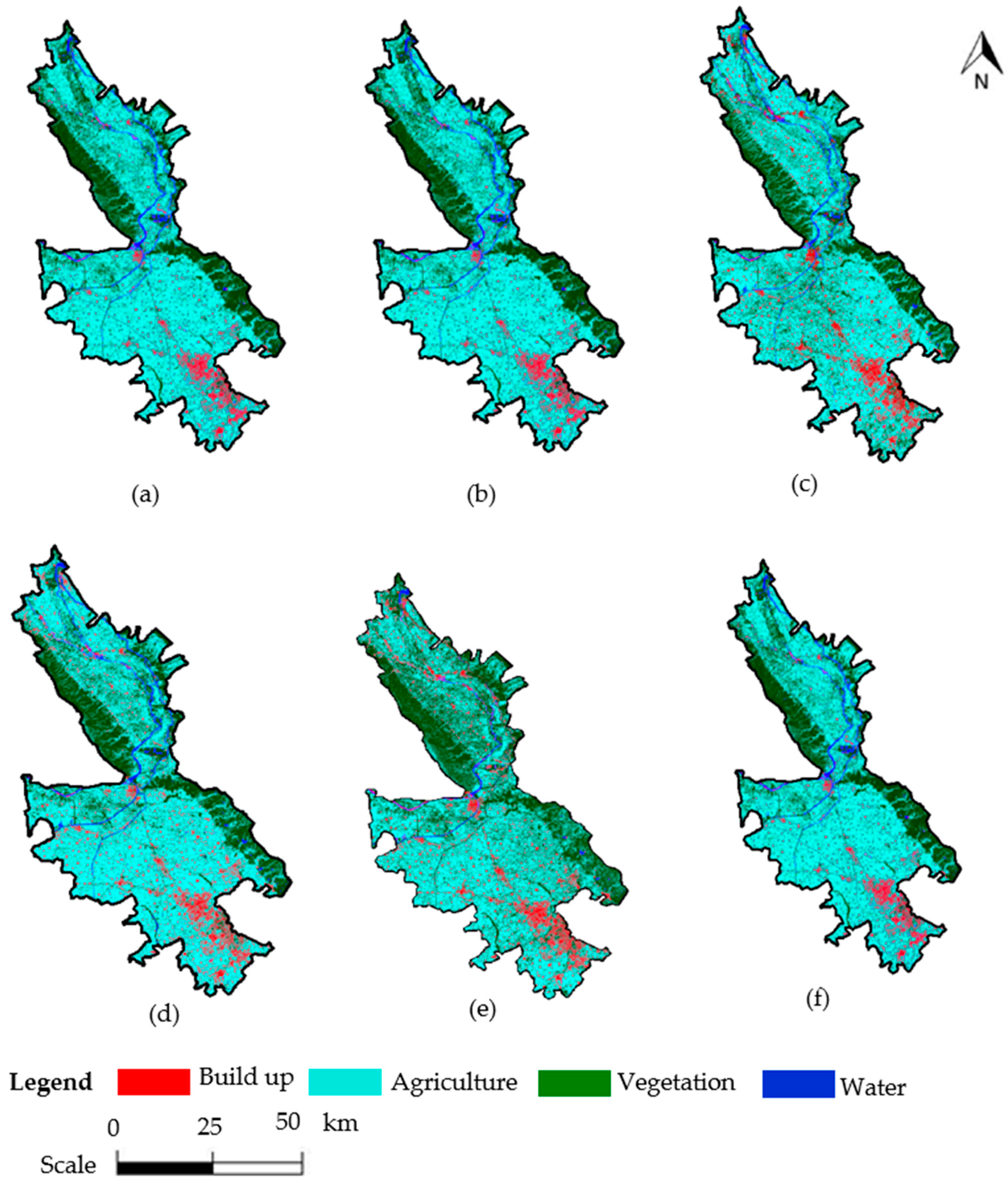
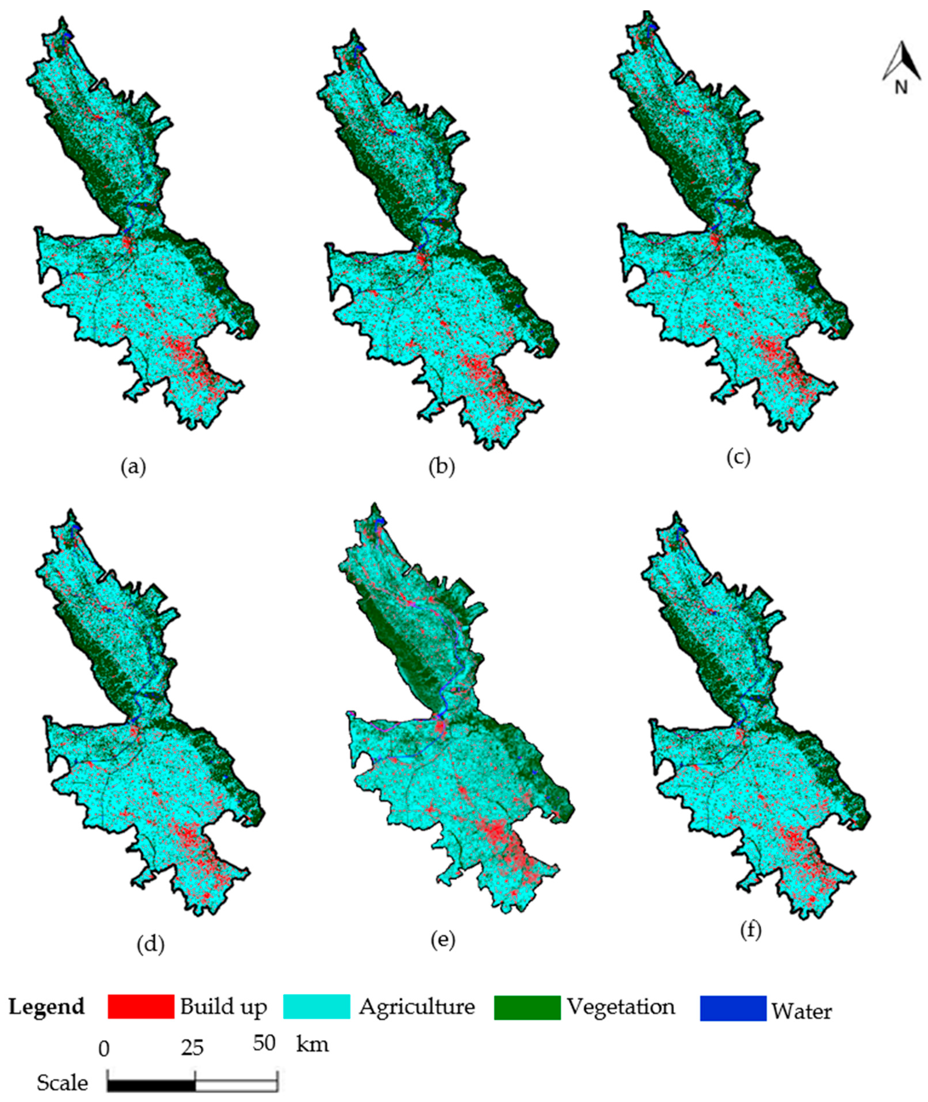
4.1. Visual Analysis of Classified Maps

The spatial variations in LULC classification maps obtained from Landsat-8 images through five classifiers are represented in Figure 4, namely, Hy-DNN, RF, CART, MDC, NB, and CNN, exposing clear differences in accuracy and homogeneity at the spatial level.

The Hy-DNN classifier, as shown in Figure 4a, gives the most visually consistent result, with well-defined delineation of vegetation in the northern and northeastern vegetation regions, correct mapping of agricultural zones in the central and southern regions, and detection of built-up and waterbody regions. The classification looks smooth with negligible pixel-level noise or misclassification. The RF classifier in Figure 4b is good, especially in separating vegetation and agricultural land. Built-up features are accurately tagged, with some minor over-classification in dispersed zones. Waterbodies are detected with acceptable accuracy but are underrepresented compared with Hy-DNN. The CART classifier (Figure 4c) generates fairly accurate output but shows noticeable confusion between farming and vegetation classes, particularly at border areas. Built-up features can be identified, but are more fragmented, whereas water classification is satisfactory, though less clear-cut than with RF.

Conversely, the MDC classifier in Figure 4d adds more noise to the classification. Built-up areas are generalised and overextended at times, while the vegetation and agriculture zones lack clear boundaries. Waterbody classification is also unsupportive. The NB classifier, as evident in Figure 4e, has the least accurate output, which is typified by high intermixing of the classes. Agricultural and built-up zones are not well differentiated, vegetation is under-classified, and water bodies are misclassified. Figure 4f shows that the CNN classifier delivers moderately accurate results, though not as smooth as those of Hy-DNN. Vegetation and agriculture are reasonably well-separated, but pixel-level noise is visible in some transition zones. Detection of built-up areas is satisfactory, but some patches appear noisy. Waterbodies are present but narrower and less continuous compared to Hy-DNN. Generally speaking, a visual assessment supports Hy-DNN’s better performance in maintaining high spatial accuracy and class discrimination than CNN, RF, CART, MDC, and NB, with higher confusion and classification noise. These observations correspond to the quantitative accuracy results and demonstrate the efficiency of Hy-DNN in LULC mapping with Landsat-8.

The mappings in Figure 5 derived from Sentinel-2 imagery and five different algorithms—Hy-DNN, RF, CART, MDC, NB, and CNN— show striking variations in spatial detail and classification correctness. Of these, the Hy-DNN model (Figure 5a) provides the most correct and consistent classification, successfully identifying dense vegetation in the northern part, extensive agricultural fields, and sharply delineated built-up and waterbody areas. It is visually clean with little noise or class overlap, demonstrating the model’s high capacity to leverage Sentinel-2’s high-resolution data. Hy-DNN shows good performance regarding the detection of vegetation and water bodies, but there is slight confusion at the edges of agricultural and built-up regions.

The CART classifier, Figure 5c, is reasonably good but shows more mixed pixels between agriculture and vegetation and partly fragmented built-up regions. In contrast, the MDC classifier (Figure 5d) demonstrates moderate classification quality with increased overlap between agriculture and vegetation classes, resulting in less clear land cover boundaries. The NB classifier in Figure 5e has the worst performance, with significant misclassification between built-up and agricultural regions, and poor modeling of vegetation. Waterbodies are also less uniformly detected. CNN classifier (Figure 5f) captures the major land cover types but suffers from spatial noise and irregularity in class boundaries. Built-up zones appear scattered, and water features are discontinuous, indicating a need for further model refinement.

4.2. Statistical Analysis of Classified Maps

The statistical analysis of Sentinel-2 for classification accuracy parameters describe in

Table 2. Statistical analysis of implementation of (a) NB, (b) MDC, (c) CART, (d) RF, (e) Hyper-tuned DNN, and (f) CNN using Sentinel-2.

		Accuracy Parameters
Classifier	Classified Data	PA	CA	Kc	OA
NB	Agriculture	0.82	0.85	83.00%	85.00%
	Vegetation	0.53	0.96
	Built-up	0.86	0.83
	Waterbody	0.8	0.8
MDC	Agriculture	0.92	0.97	85.00%	87.00%
	Vegetation	0.84	0.96
	Built-up	0.97	0.93
	Waterbody	0.82	0.83
CART	Agriculture	0.9	0.9	89.00%	90.00%
	Vegetation	0.93	0.92
	Built-up	0.89	0.85
	Waterbody	0.86	0.87
RF	Agriculture	0.84	0.92	91.00%	92.00%
	Vegetation	0.89	0.91
	Built-up	0.94	0.93
	Waterbody	0.93	0.94
Hyper-tuned DNN	Agriculture	0.96	1	96.80%	97.60%
	Vegetation	0.99	0.95
	Built-up	0.97	0.96
	Waterbody	0.96	0.98
CNN	Agriculture	0.91	0.96	94.00%	95.23%
	Vegetation	0.97	0.89
	Built-up	0.92	0.92
	Waterbody	0.91	0.93

. reveals that the Hyper-tuned Deep Neural Network (DNN) outperforms all other classifiers, achieving the highest overall accuracy (97.60%) and Kappa coefficient (96.80%). It demonstrates exceptional precision across all land cover classes, particularly for agriculture (PA = 0.96, CA = 1.00) and vegetation (PA = 0.99, CA = 0.95). The Convolutional Neural Network (CNN) also shows strong performance with an overall accuracy of 95.23% and Kappa coefficient of 94.00%, although slightly lower consumer’s accuracy for vegetation (0.89) suggests minor classification confusion. The Hyper-tuned DNN outperforms the CNN model across all land cover classes, particularly for agriculture (Kc 0.91 vs. 0.88) and vegetation (0.88 vs. 0.85). The overall accuracy and Kc are also higher for Hy-DNN (91.10% and 88.10%) compared to CNN (88.13% and 87.23%), indicating improved classification precision and robustness.

Among traditional classifiers, Random Forest (RF) achieves the best performance, with 92.00% overall accuracy and a Kappa coefficient of 91.00%. It provides consistently high PA and CA across all classes, particularly waterbody (PA = 0.93, CA = 0.94) and built-up (PA = 0.94, CA = 0.93). CART follows closely, offering balanced results with 90.00% overall accuracy and high accuracy for Vegetation (PA = 0.93, CA = 0.92). The Minimum Distance Classifier (MDC) also performs well, especially for built-up (PA = 0.97), but trails slightly behind in overall performance.

Conversely, the Naive Bayes (NB) classifier records the lowest accuracy, with 85.00% OA and 83.00% Kappa. While it achieves high consumer’s accuracy for vegetation (0.96), its low producer’s accuracy (0.53) for the same class indicates significant omission errors. Overall, the results clearly indicate that deep learning models, particularly the Hyper-tuned DNN, offer superior performance in land use/land cover classification tasks compared to traditional machine learning approaches.

Using Landsat-8 imagery, the classification accuracy analysis highlights the performance of various machine learning and deep learning classifiers across four major land cover classes: agriculture, vegetation, built-up, and waterbody. The Hyper-tuned Deep Neural Network (DNN) emerges as the top-performing model with the highest overall accuracy (91.10%) and Kappa coefficient (88.10%) as shown in

Table 3. Qualitative analysis of the implementation of NB, MDC, CART, RF, Hy-DNN, and CNN using the Landsat-8 dataset.

		Accuracy Parameters
Classifier	Classified Classes	PA	CA	Kc	OA
NB	Agriculture	0.93	0.66	69.00%	77.00%
	Vegetation	0.31	0.83
	Built-up	0.82	0.94
	Waterbody	0.94	0.7
MDC	Agriculture	0.93	0.82	76.39%	82.25%
	Vegetation	0.43	0.87
	Built-up	1	0.94
	Waterbody	0.92	0.68
CART	Agriculture	1	0.88	85.00%	87.00%
	Vegetation	0.87	0.93
	Built-up	0.83	0.91
	Waterbody	0.92	1
RF	Agriculture	1	0.88	87.00%	88.00%
	Vegetation	0.87	0.93
	Built-up	0.81	0.83
	Waterbody	0.92	0.82
Hyper-tuned DNN	Agriculture	0.88	0.92	88.10%	91.10%
	Vegetation	0.9	0.88
	Built-up	0.93	0.9
	Waterbody	0.92	0.94
CNN	Agriculture	0.87	0.9	87.23%	88.13%
	Vegetation	0.88	0.85
	Built-up	0.92	0.89
	Waterbody	0.9	0.93

. It demonstrates balanced and robust classification performance across all classes, with producer’s accuracy (PA) and consumer’s accuracy (CA) exceeding 0.88 for each class. Notably, it excels in classifying built-up (PA = 0.93, CA = 0.90) and waterbody (PA = 0.92, CA = 0.94), indicating its superior generalisation and minimal misclassification.

The Convolutional Neural Network (CNN) also shows strong results, achieving an overall accuracy of 88.13% and a Kappa coefficient of 87.23%. It maintains high accuracy across all classes as compared to traditional classifiers, especially in built-up (PA = 0.92, CA = 0.89) and waterbody (PA = 0.90, CA = 0.93). Among traditional classifiers, Random Forest (RF) stands out with an 88.00% overall accuracy and 87.00% Kappa coefficient, closely competing with CNN. RF demonstrates excellent performance for agriculture (PA = 1.00) and vegetation (CA = 0.93), but slightly lower accuracy for built-up, compared to deep learning models.

The CART classifier also performs competitively, with 87.00% overall accuracy and 85.00% Kappa. It is particularly effective in classifying waterbody (CA = 1.00) and vegetation (PA = 0.87, CA = 0.93). On the other hand, the Minimum Distance Classifier (MDC) and Naive Bayes (NB) lag behind, with NB showing the weakest performance (OA = 77.00%, Kc = 69.00%). NB suffers from particularly low vegetation PA (0.31), indicating high omission errors. MDC performs slightly better (OA = 82.25%, Kc = 76.39%) but still falls short of the advanced classifiers.

5. Discussion

In the current research, two multispectral satellite datasets—Sentinel-2 and Landsat-8—were utilised for carrying out land use and land cover (LULC) classification to evaluate the effect on agricultural production land in Punjab’s Rupnagar district, India, with food security planning implications. These five classifiers, namely machine learning and deep learning-based classifiers such as Random Forest (RF), Classification and Regression Tree (CART), Minimum Distance Classifier (MDC), Naive Bayes (NB), Convolution Neural Network (CNN) and Hyper-tuned Deep Neural Network (Hy-DNN), were used in combination. Their performance was compared with existing research that utilised classification methods on the Google Earth Engine (GEE) platform, RF, and CART. Those studies yielded overall accuracies (OA) of 87.99%, 87.81%, and 84.72%, respectively. A study based on CART for the classification of water, urban, tree, and ground classes attained an accuracy of 92.9%. For comparison, the Hy-DNN model in this study showed better performance with greater accuracy measures. Accuracy measures for Sentinel-2 and Landsat-8 datasets are presented in Figure 6.

In contrast to previous research [5], which employed a narrow spectrum of spectral bands—commonly RGB and NIR—the current research included the red-edge spectral band (Band 5) of Sentinel-2, which has been found to considerably improve vegetation classification accuracy [5]. In addition, whereas the 30 m spatial resolution of Landsat-8 placed constraints on the detection of fine-scale land cover change in urban and mixed-use landscapes [7], the employment of higher resolution Sentinel-2 imagery (10 m) enabled more precise and detailed mapping of complexly structured landscapes. Earlier studies relied on single or double classification methods and did not have strong quantitative validation, with little application of accuracy measures like confusion matrix, OA, and Kappa coefficient (KC) [8,44]. This study, however, built a comprehensive confusion matrix for all the classifiers for every land cover class and computed both OA and KC. These measures enabled a statistically sound evaluation framework and facilitated easier inter-model comparisons as well as more confidence in the results of the classifications.

Although previous research attained maximum accuracies of 90.6% [45], 92.53% [46], and 92.2% (with some class-specific accuracies as low as 14%), the Hy-DNN model herein outperformed them, with an OA of 97.60% and a higher class-specific accuracy [9,12]. This study also employed a larger validation sample size (1000 samples), unlike previous studies that employed only 160 samples [11]. In contrast to other methods that heavily relied on external data sources like DEM, NDVI, and post-classification correction (PCC) for enhancing the low accuracy of classifying approaches like the Maximum Likelihood Classifier (MLC) [15], the current research employed a stronger and more inclusive classification approach. By integrating several advanced classifiers—such as Hy-DNN, MDC, NB, RF, and CART—this research attained high accuracy in classification without too much use of post-processing procedures.

To further validate Hy-DNN performance, it is compared with other studies that implemented classification on GEE using SVM, RF, and CART classifiers. The OA of SVM, RF, and CART was 87.99%, 87.81%, and 84.72%, respectively. Another study using CART on GEE for classifying water, urban, tree, and ground classes reported an accuracy of 92.9% [45]. In comparison, Hy-DNN demonstrates superior performance. Figure 6 represents the accuracy assessment results using Sentinel-2 and Landsat-8 satellite data.

The Hy-DNN framework shows optimised results with an accuracy of 97.60% in the case of Sentinel-2 and 91.10% using Landsat-8 multispectral datasets, compared to the other machine learning classifiers. Figure 5 shows the comparison of different classifiers using the Sentinel-2 (10 m) dataset, and Figure 4 shows the accuracy assessment using the Landsat-8 dataset. A confusion matrix shows the quantitative analysis of the study. The Hy-DNN model distinguishes itself from conventional deep neural networks by utilising a hybrid architecture that integrates both shallow and deep layers, effectively balancing computational efficiency with improved feature extraction.

It features a systematic hyperparameter tuning process aimed at optimising critical parameters such as learning rate, momentum, and the number of neurons in hidden layers, which enhances classification accuracy. Unlike traditional models that operate with static configurations, the Hy-DNN is specifically tailored for remote sensing applications, making it adept at capturing the intricate spectral and spatial characteristics of multispectral imagery. This targeted approach for agricultural land classification embodies the model’s primary innovation. From both the visual and statistical analyses, it can be concluded that the Hy-DNN algorithm can classify LULC with better accuracy compared to RF, MDC, CART, and NB.

The Hyper-tuned Deep Neural Network (Hy-DNN) demonstrates superior performance over all other classifiers, as shown in

Table 4. Comparison table between Hy-DNN and common QGIS/ArcGIS methods.

Classifier	Sentinel-2 (Kc/OA)	Landsat-8 (Kc/OA)	Scalability	Usability in QGIS/ArcGIS
NB	Kc = 83% OA = 85%	Kc = 69% OA = 77%	Very High (lightweight, fast)	Fully integrated in QGIS (SCP) and ArcGIS; easy to use
MDC	Kc = 85% OA = 87%	Kc = 76% OA = 82%	High (low memory, but sensitive to stats)	Available in QGIS/ArcGIS via classification toolsets
CART	Kc = 89% OA = 90%	Kc = 85% OA = 87%	High (interpretable and fast training)	Built in GEE, QGIS (SCP), and ArcGIS Model Builder
RF	Kc = 91% OA = 92%	Kc = 87% OA = 88%	Very High (robust, scalable with ensemble)	Fully supported in QGIS (SCP) and ArcGIS (Classifier tool)
CNN	Kc = 88% OA = 91%	Kc = 94% OA = 95%	High (requires GPU, scalable for moderate datasets)	Limited native support; requires integration via Python (3.9.11) or deep learning plugins in GEE or custom QGIS tools
Hyper-tuned DNN	Kc = 96% OA = 97%	Kc = 88% OA = 91%	Very High (best for large, complex datasets; requires tuning and training resources)	Not natively supported in QGIS/ArcGIS; requires GEE, Python, TensorFlow

, achieving the highest values for both Kappa coefficient and overall accuracy for both Sentinel-2 and Landsat 8 datasets. In contrast, traditional classifiers such as Random Forest (RF) and Classification and Regression Trees (CART) are readily accessible within platforms like QGIS (3.34) and ArcGIS (10.8.2), making them more user-friendly and suitable for practitioners with limited expertise in deep learning. While the Hy-DNN offers excellent scalability and advanced customization capabilities, its implementation requires integration with external tools such as Google Earth Engine (GEE) and machine learning frameworks like TensorFlow or Keras capabilities, which are not natively supported in QGIS/ArcGIS environments.

The comparison between Landsat-8 and Sentinel-2 datasets in Figure 6 demonstrates that Sentinel-2 offers superior performance in land use/land cover (LULC) classification, mainly due to its higher spatial resolution (10 m) and more frequent revisit interval (5 days). These characteristics allow for clearer boundary delineation and better distinction between complex classes, such as agriculture and built-up areas. Deep learning models, especially the Hyper-tuned DNN, consistently outshine traditional classifiers, achieving a top overall accuracy of 97.60% and a Kappa coefficient of 96.80% with Sentinel-2, compared to 91.10% using Landsat-8. CNN also delivered strong, balanced results with minimal errors. Although traditional methods like RF and CART showed acceptable performance, they lacked the consistency and precision of deep learning approaches. Overall, integrating Sentinel-2 imagery with advanced deep learning techniques proves to be the most effective strategy for accurate and detailed LULC mapping, particularly in diverse agricultural landscapes such as Rupnagar.

The confusion matrix heatmaps [46,47,48] illustrate the performance of five different classification algorithms, Hy-DNN, RF, CART, MDC, NB, and CNN, applied to Sentinel-2 satellite imagery for land cover classification across four classes, vegetation, built-up, waterbody, and agriculture, as shown in Figure 7a–f. Among all models, Hy-DNN achieved the most balanced and accurate classification across all classes, with minimal misclassifications, demonstrating its strength in handling the complex spectral information provided by Sentinel-2 [46].

The RF and CART classifiers also performed well, especially in identifying the agriculture class with high accuracy, though they showed some confusion between vegetation and built-up classes. While reasonably effective for agriculture and waterbody, the MDC and NB classifiers struggled more with distinguishing vegetation and built-up classes, indicating their limitations in handling mixed or overlapping spectral signatures. The Figure 7i matrix shows that the CNN model performs very well, with high values on the diagonal, especially for the agriculture and waterbody classes, indicating accurate predictions. Misclassifications are low and more evenly distributed compared to RF, reflecting CNN’s better feature extraction capacity. The Sentinel-2 dataset, with its high-resolution multispectral bands, proves to be highly effective for land cover classification, especially when used with advanced deep learning techniques like Hy-DNN, which can fully leverage the data’s richness and variability.

Figure 7g–l display confusion matrix heatmaps for six classification algorithms—Hy-DNN, RF, CART, MDC, NB, and CNN—applied to Landsat-8 satellite imagery for land cover classification across four classes: water, built-up, vegetation, and agriculture. These matrices offer insight into each classifier’s ability to distinguish land cover types based on the spectral features of Landsat-8. The Hy-DNN classifier demonstrates robust performance across all classes, with high accuracy in classifying water (235), built-up (226), vegetation (220), and agriculture (230) classes, though some confusion exists between vegetation and agriculture classes. RF achieves strong classification performance, especially for vegetation (242) and waterbody (274) classes, but slightly underperforms for agriculture (210), with some misclassification into the built-up class.

CART shows nearly perfect classification for water and vegetation classes, though it shares RF’s trend of minor errors in agriculture prediction. MDC performs well for waterbody (274) and moderately for vegetation (226), but shows notable confusion between built-up and agriculture classes, with a large portion of built-up misclassified as agriculture (97 instances). NB is the weakest performer among the five. It struggles significantly with built-up and agriculture, misclassifying substantial portions of these classes into each other, although it still performs adequately on the waterbody and vegetation classes. The CNN classifier confusion matrix demonstrates high classification accuracy across all land cover classes, with strong diagonal values indicating reliable predictions. Minor misclassifications are evenly distributed, reflecting the model’s robustness and superior generalisation compared to traditional classifiers.

6. Conclusions

In this study, multispectral data from Landsat-8 and Sentinel-2 were analyzed over the Rupnagar region in Punjab, India. The land was classified as vegetation, agriculture, water bodies, and built-up areas using various classification algorithms, including Hy-DNN, RF, CART, MDC, NB, and CNN. The study employed a Hy-DNN model, which outperformed the other classifiers, achieving 97.60% accuracy with the Sentinel-2 dataset and 91.10% accuracy with the Landsat-8 dataset. In comparison, the CNN classifier achieved 92% accuracy with Sentinel-2 and 88% with Landsat-8; the RF classifier achieved 92% accuracy with Sentinel-2 and 88% with Landsat-8; the CART classifier achieved 90% accuracy with Sentinel-2 and 88.7% with Landsat-8; while the MDC achieved 87% with Sentinel-2 and 82.25% with Landsat-8. The NB classifier yielded 85% accuracy with Sentinel-2 and 77% with Landsat-8. The findings suggest that the Hy-DNN model is highly optimized for land classification tasks. The limitation of this study is that, while the hybrid architecture improves feature extraction, it also introduces increased computational complexity. Training Hy-DNN requires significantly more processing power and memory, making it less practical for applications in resource-constrained environments or for real-time analysis. Future applications of this research could include crop health monitoring, disease detection, and crop growth analysis in various regions.

References

1. Sharma, I.; Kaur, K. Datasets for Satellite Remote Sensing in Agriculture: An Overview and Analysis. In Proceedings of the 2024 3rd Edition of IEEE Delhi Section Flagship Conference (DELCON), New Delhi, India, 21–23 November 2024; pp. 1–7. [Google Scholar] [CrossRef]
2. Colliander, A.; Fisher, J.B.; Halverson, G.; Merlin, O.; Misra, S.; Bindlish, R.; Jackson, T.J.; Yueh, S. Spatial Downscaling of SMAP Soil Moisture Using MODIS Land Surface Temperature and NDVI during SMAPVEX15. IEEE Geosci. Remote Sens. Lett. 2017, 14, 2107–2111. [Google Scholar] [CrossRef]
3. Boonman, C.C.F.; Heuts, T.S.; Vroom, R.J.E.; Geurts, J.J.M.; Fritz, C. Wetland Plant Development Overrides Nitrogen Effects on Initial Methane Emissions after Peat Rewetting. Aquat. Bot. 2023, 184, 103598. [Google Scholar] [CrossRef]
4. Sharma, N.; Chawla, S. Digital Change Detection Analysis Criteria and Techniques Used for Land Use and Land Cover Classification in Agriculture. In Proceedings of the 2023 3rd International Conference on Advance Computing and Innovative Technologies in Engineering (ICACITE), Greater Noida, India, 12 May 2023; pp. 331–335. [Google Scholar] [CrossRef]
5. Saini, R.; Singh, S. Land Use Land Cover Classification Using Machine Learning and Remote Sensing Data: A Case Study of Karnaprayag, Uttarakhand, India. In Proceedings of the 2024 First International Conference on Electronics, Communication and Signal Processing (ICECSP), New Delhi, India, 8–10 August 2024; pp. 1–6. [Google Scholar]
6. Zhao, Q.; Yu, L.; Li, X.; Peng, D.; Zhang, Y.; Gong, P. Progress and Trends in the Application of Google Earth and Google Earth Engine. Remote Sens. 2021, 13, 3778. [Google Scholar] [CrossRef]
7. Chowdhury, A.; Dwarakish, G.S. Selection of Algorithm for Land Use Land Cover Classification and Change Detection. IJARSCT 2022, 2, 15–24. [Google Scholar] [CrossRef]
8. Mahdi, A.S. The Land Use and Land Cover Classification on the Urban Area. Iraqi J. Sci. 2022, 66, 4609–4619. [Google Scholar] [CrossRef]
9. Thaiki, M.; Bounoua, L.; Cherkaoui Dekkaki, H. Using Satellite Data to Characterize Land Surface Processes in Morocco. Remote Sens. 2023, 15, 5389. [Google Scholar] [CrossRef]
10. Santos, M.P.; Prado, L.A.D.S.; Cogo, A.J.D.; Lopes, A.V.S.; Caldeira, C.F.; Cavalcante, A.B.; Martins, R.L.; de Assis Esteves, F.; Duarte, H.M.; Zandonadi, D.B. High Irradiance Impairs Isoëtes Cangae Growth. Aquat. Bot. 2023, 184. [Google Scholar] [CrossRef]
11. Jasim, B.S.; Jasim, O.Z.; AL-Hameedawi, A.N. Evaluating Land Use Land Cover Classification Based on Machine Learning Algorithms. Eng. Technol. J. 2024, 42. [Google Scholar] [CrossRef]
12. Chomani, K.; Pshdari, S. Evaluation of Different Classification Algorithms for Land Use Land Cover Mapping. Kurdistan J. Appl. Res. 2024, 9, 13–22. [Google Scholar] [CrossRef]
13. Kussul, N.; Lavreniuk, M.; Skakun, S.; Shelestov, A. Deep Learning Classification of Land Cover and Crop Types Using Remote Sensing Data. IEEE Geosci. Remote Sens. Lett. 2017, 14, 778–782. [Google Scholar] [CrossRef]
14. Srivastav, A.L.; Dhyani, R.; Ranjan, M.; Madhav, S.; Sillanpää, M. Climate-Resilient Strategies for Sustainable Management of Water Resources and Agriculture. Environ. Sci. Pollut. Res. 2021, 28, 41576–41595. [Google Scholar] [CrossRef] [PubMed]
15. Manandhar, R.; Odehi, I.O.A.; Ancevt, T. Improving the Accuracy of Land Use and Land Cover Classification of Landsat Data Using Post-Classification Enhancement. Remote Sens. 2009, 1, 330. [Google Scholar] [CrossRef]
16. Mhanna, S.; Halloran, L.J.S.; Zwahlen, F.; Asaad, A.H.; Brunner, P. Using Machine Learning and Remote Sensing to Track Land Use/Land Cover Changes Due to Armed Conflict. Sci. Total Environ. 2023, 898, 165600. [Google Scholar] [CrossRef]
17. Celebrezze, J.V.; Alegbeleye, O.M.; Glavich, D.A.; Shipley, L.A.; Meddens, A.J.H. Classifying Rocky Land Cover Using Random Forest Modeling: Lessons Learned and Potential Applications in Washington, USA. Remote Sens. 2025, 17, 915. [Google Scholar] [CrossRef]
18. Aberle, R.; Enderlin, E.; O’Neel, S.; Florentine, C.; Sass, L.; Dickson, A.; Marshall, H.-P.; Flores, A. Automated Snow Cover Detection on Mountain Glaciers Using Spaceborne Imagery and Machine Learning. Cryosphere 2025, 19, 1675–1693. [Google Scholar] [CrossRef]
19. Zeferino, L.B.; de Souza, L.F.T.; Amaral, C.H.D.; Filho, E.I.F.; de Oliveira, T.S. Does Environmental Data Increase the Accuracy of Land Use and Land Cover Classification? Int. J. Appl. Earth Obs. Geoinf. 2020, 91, 102128. [Google Scholar] [CrossRef]
20. Ayushi; Buttar, P.K. Satellite Imagery Analysis for Crop Type Segmentation Using U-Net Architecture. Procedia Comput. Sci. 2024, 235, 3418–3427. [Google Scholar] [CrossRef]
21. Luo, K.; Lu, L.; Xie, Y.; Chen, F.; Yin, F.; Li, Q. Crop Type Mapping in the Central Part of the North China Plain Using Sentinel-2 Time Series and Machine Learning. Comput. Electron. Agric. 2023, 205, 107577. [Google Scholar] [CrossRef]
22. Latif, B.A.; Lecerf, R.; Mercier, G.; Hubert-Moy, L. Preprocessing of Low-Resolution Time Series Contaminated by Clouds and Shadows. IEEE Trans. Geosci. Remote Sens. 2008, 46, 2083–2096. [Google Scholar] [CrossRef]
23. Kluger, D.M.; Wang, S.; Lobell, D.B. Two Shifts for Crop Mapping: Leveraging Aggregate Crop Statistics to Improve Satellite-Based Maps in New Regions. Remote Sens. Environ. 2021, 262, 112488. [Google Scholar] [CrossRef]
24. Marujo, R.F.B.; Fronza, J.G.; Soares, A.R.; Queiroz, G.R.; Ferreira, K.R. Evaluating the Impact of Lasrc and Sen2cor Atmospheric Correction Algorithms on Landsat-8/Oli and Sentinel-2/Msi Data Over Aeronet Stations in Brazilian Territory. ISPRS Ann. Photogramm. Remote Sens. Spat. Inf. Sci. 2021, 3, 271–277. [Google Scholar] [CrossRef]
25. Mandal, D.; Kumar, V.; Bhattacharya, A.; Rao, Y.S.; Siqueira, P.; Bera, S. Sen4Rice: A Processing Chain for Differentiating Early and Late Transplanted Rice Using Time-Series Sentinel-1 SAR Data with Google Earth Engine. IEEE Geosci. Remote Sens. Lett. 2018, 15, 1947–1951. [Google Scholar] [CrossRef]
26. Jamal, S.; Ahmad, W.S. Assessing Land Use Land Cover Dynamics of Wetland Ecosystems Using Landsat Satellite Data. SN Appl. Sci. 2020, 2, 1–24. [Google Scholar] [CrossRef]
27. Vyas, N.; Singh, S.; Sethi, G.K. A Novel Image Fusion-Based Post Classification Framework for Agricultural Variations Detection Using Sentinel-1 and Sentinel-2 Data. Earth Sci. Inform. 2025, 18. [Google Scholar] [CrossRef]
28. Singh, G.; Dahiya, N.; Sood, V.; Singh, S.; Sharma, A. ENVINet5 Deep Learning Change Detection Framework for the Estimation of Agriculture Variations during 2012–2023 with Landsat Series Data. Environ. Monit. Assess. 2024, 196, 233–245. [Google Scholar] [CrossRef]
29. Talukdar, S.; Singha, P.; Mahato, S.; Shahfahad; Pal, S.; Liou, Y.A.; Rahman, A. Land-Use Land-Cover Classification by Machine Learning Classifiers for Satellite Observations-A Review. Remote Sens. 2020, 12, 1135. [Google Scholar] [CrossRef]
30. Li, Y.; Liu, C.; Zhang, J.; Zhang, P.; Xue, Y. Monitoring Spatial and Temporal Patterns of Rubber Plantation Dynamics Using Time-Series Landsat Images and Google Earth Engine. IEEE J. Sel. Top. Appl. Earth Obs. Remote Sens. 2021, 14, 9450–9461. [Google Scholar] [CrossRef]
31. Setiawan, M.D.; Setiawan, E.B. Machine Learning Method for Carbon Stock Classification with Drone and GEE Data. In Proceedings of the 2025 International Conference on Advancement in Data Science, E-learning and Information System (ICADEIS), Bandung, Indonesia, 3–4 February 2025; pp. 1–7. [Google Scholar]
32. Ravirathinam, P.; Ghosh, R.; Khandelwal, A.; Jia, X.; Mulla, D.; Kumar, V. Combining Satellite and Weather Data for Crop Type Mapping: An Inverse Modelling Approach. In Proceedings of the 2024 SIAM International Conference on Data Mining (SDM), Houston, TX, USA, 18–20 April 2024; pp. 445–453. [Google Scholar] [CrossRef]
33. Kafle, S.; Sandeep, K.C.; Poudyal, B.; Devkota, S. Machine Learning Approach to Detect Land Use Land Cover (LULC) Change in Chure Region of Sarlahi District, Nepal. Arch. Agric. Environ. Sci. 2023, 8, 168–174. [Google Scholar] [CrossRef]
34. De Oliveira, J.P.; Costa, M.G.F.; Costa Filho, C.F.F. Methodology of Data Fusion Using Deep Learning for Semantic Segmentation of Land Types in the Amazon. IEEE Access 2020, 8, 187864–187875. [Google Scholar] [CrossRef]
35. Xie, G.; Niculescu, S. Mapping and Monitoring of Land Cover/Land Use (LCLU) Changes in the Crozon Peninsula (Brittany, France) from 2007 to 2018 by Machine Learning Algorithms (Support Vector Machine, Random Forest, and Convolutional Neural Network) and by Post-Classification Comparison (PCC). Remote Sens. 2021, 13, 3899. [Google Scholar] [CrossRef]
36. Jamali, A. Evaluation and Comparison of Eight Machine Learning Models in Land Use/Land Cover Mapping Using Landsat 8 OLI: A Case Study of the Northern Region of Iran. SN Appl. Sci. 2019, 1, 1448. [Google Scholar] [CrossRef]
37. Singh, S.; Tiwari, R.K.; Gusain, H.S.; Sood, V. Potential Applications of SCATSAT-1 Satellite Sensor: A Systematic Review. IEEE Sens. J. 2020, 20, 12459–12471. [Google Scholar] [CrossRef]
38. Basheer, S.; Wang, X.; Farooque, A.A.; Nawaz, R.A.; Liu, K.; Adekanmbi, T.; Liu, S. Comparison of Land Use Land Cover Classifiers Using Different Satellite Imagery and Machine Learning Techniques. Remote Sens. 2022, 14, 4978. [Google Scholar] [CrossRef]
39. Srivastava, A.; Bharadwaj, S.; Dubey, R.; Sharma, V.B.; Biswas, S. Mapping Vegetation and Measuring the Performance of Machine Learning Algorithm in Lulc Classification in the Large Area Using Sentinel-2 and Landsat-8 Datasets of Dehradun as a Test Case. Int. Arch. Photogramm. Remote Sens. Spat. Inf. Sci. 2022, 43, 529–535. [Google Scholar] [CrossRef]
40. Gøttcke, J.M.N.; Zimek, A.; Campello, R.J.G.B. Bayesian Label Distribution Propagation: A Semi-Supervised Probabilistic k Nearest Neighbor Classifier. Inf. Syst. 2025, 129, 102507. [Google Scholar] [CrossRef]
41. Jackins, V.; Vimal, S.; Kaliappan, M.; Lee, M.Y. AI-Based Smart Prediction of Clinical Disease Using Random Forest Classifier and Naive Bayes. J. Supercomput. 2021, 77, 5198–5219. [Google Scholar] [CrossRef]
42. He, Y.; Ou, G.; Fournier-Viger, P.; Huang, J.Z. Attribute Grouping-Based Naive Bayesian Classifier. Sci. China Inf. Sci. 2025, 68, 132106. [Google Scholar] [CrossRef]
43. Liu, T.; Yang, L.; Lunga, D. Change Detection Using Deep Learning Approach with Object-Based Image Analysis. Remote Sens. Environ. 2021, 256, 112308. [Google Scholar] [CrossRef]
44. Dahiya, N.; Singh, S.; Gupta, S. Comparative Analysis and Implication of Hyperion Hyperspectral and Landsat-8 Multispectral Dataset in Land Classification. J. Indian Soc. Remote Sens. 2023, 51, 2201–2213. [Google Scholar] [CrossRef]
45. Waghela, H.; Patel, S.; Sudesan, P.; Raorane, S.; Borgalli, R. Land Use Land Cover Classification Using Machine Learning. In Proceedings of the 2022 International Conference on Automation, Computing and Renewable Systems (ICACRS), Pudukkottai, India, 13–15 December 2022; pp. 708–711. [Google Scholar]
46. Fan, C.-L. Evaluation Model for Crack Detection with Deep Learning: Improved Confusion Matrix Based on Linear Features. J. Constr. Eng. Manag. 2025, 151, 4024210. [Google Scholar] [CrossRef]
47. Jiang, Y.; Liu, Z.; Kabirzadeh, P.; Wu, Y.; Li, Y.; Miljkovic, N.; Wang, P. Multi-Fidelity Physics-Informed Convolutional Neural Network for Heat Map Prediction of Battery Packs. Reliab. Eng. Syst. Saf. 2025, 256, 110752. [Google Scholar] [CrossRef]
48. Amani, M.; Ghorbanian, A.; Ahmadi, S.A.; Kakooei, M.; Moghimi, A.; Mirmazloumi, S.M.; Moghaddam, S.H.A.; Mahdavi, S.; Ghahremanloo, M.; Parsian, S.; et al. Google Earth Engine Cloud Computing Platform for Remote Sensing Big Data Applications: A Comprehensive Review. IEEE J. Sel. Top. Appl. Earth Obs. Remote Sens. 2020, 13, 5326–5350. [Google Scholar] [CrossRef]
Figure 1. Representation of the study area. (a) The India map highlights the Punjab state. (b) The Punjab map highlights Rupnagar. (c) Satellite dataset file for Rupnagar (RGB: NIR-Red-Green).
Land 14 01578 g001
Figure 2. (a) Framework for implementation of the Hy-DNN model. (b) Workflow of (i) traditional GIS, and (ii) Hy-DNN model.
Land 14 01578 g002
Figure 3. (a) Layered architecture of Hy-DNN with hyper-tuned parameters. (b) Flow chart for implementing RF, CART, MDC, NB, and CNN.
Land 14 01578 g003aLand 14 01578 g003b
Figure 4. Qualitative analysis of (a) Hy-DNN, (b) RF, (c) CART, (d) MDC, (e) NB, and (f) CNN using Landsat-8.
Land 14 01578 g004
Figure 5. Qualitative analysis of (a) Hy-DNN, (b) RF, (c) CART, (d) MDC, (e) NB, and (f) CNN using Sentinel-2.
Land 14 01578 g005
Figure 6. Accuracy comparison of Landsat-8 and Sentinel-2 with different classifiers.
Land 14 01578 g006
Figure 7. Heatmap of different classifiers using satellite datasets (af) Sentinel-2, and (gl) Landsat-8.
Land 14 01578 g007