Spatiotemporal Dynamics and Drivers of Ecological Carrying Capacity in the Dongting Lake Region Using Remote Sensing and Spatial Modeling

Abstract

Ecological Carrying Capacity (ECC) represents an ecosystem’s ability to sustain human activities without compromising its ecological integrity, yet fine-scale quantification of its spatiotemporal dynamics remains limited. Focusing on the ecologically vital Dongting Lake Region (DTLR) in China, this study established a finer resolution ECC assessment framework by integrating multi-source remote sensing data within the Driving Forces–Pressure–State–Impact–Response–Management (DPSIRM) model. ECC and its driving mechanisms were examined across the DTLR and its surrounding buffer zone from 2000 to 2020. Results revealed a pronounced U-shaped trajectory of ECC in the DTLR, with an initial decline followed by a sustained recovery after 2010, while the buffer zone consistently maintained a 15–20% higher ECC throughout. Subsystem analysis indicated steady improvements in Management capacity, whereas Pressure, State, and Impact subsystems peaked mid-period before declining. Projections suggest continued ECC enhancement, reflecting rising regional resilience. Spatially, ECC patterns jointly emerged from the interaction of anthropogenic stressors and ecological restoration. Geographically weighted regression (GWR) identified proximity to green spaces as the strongest positive driver, while impervious surface (−27%) and infrastructure density (−19%) exerted significant negative effects. These findings offer a scalable, remote sensing-based framework for ecosystem-oriented spatial planning, highlighting the strategic role of green infrastructure in sustaining ecological resilience.

1. Introduction

Growing environmental pressures and intensifying resource conflicts pose major obstacles to regional sustainable development [1]. Wetlands are among the most biologically diverse ecosystems on Earth, providing several ecosystem services, including water regulation, biodiversity maintenance, and carbon sequestration, all of which are vital for ecological stability and human well-being [2,3]. As China’s second-largest freshwater lake, Dongting Lake undertakes important functions in maintaining ecological balance [4,5]. Nonetheless, wetlands are highly sensitive and dynamic ecosystems that are easily affected by external pressures and disturbances. Recently, escalating anthropogenic activities and global environmental change have intensified stress on wetland ecosystems, creating a compounding crisis with cascading ecological and socioeconomic consequences [6]. Intensifying warming and drying climatic trends have driven substantial hydrological alterations in lake systems globally, subsequently impacting ecosystem stability and the communities that depend on them [7]. Meanwhile, unsustainable anthropogenic activities—including agricultural expansion, intensive overfishing, and unregulated industrial discharge—have emerged as primary drivers of wetland ecosystem degradation in the region. Dongting Lake faced environmental deterioration once upon a time due to rapid modernization and urbanization, leading to declines in water quality and biodiversity, and ultimately hindering its long-term Ecological Carrying Capacity [8]. In response, safeguarding ecological security and ensuring the sustainable development of wetland ecosystems have become urgent priorities for economic prosperity, community resilience, and national strategic goals [9]. By systematically evaluating the Ecological Carrying Capacity, conservation strategies, resource management, and sustainable development can be better informed, while simultaneously enhancing the effectiveness of evaluation systems and application models and, more importantly, reconciling human activities with environmental protection in the future generation.

Rooted in the ecological notion of carrying capacity, ECC traditionally refers to the threshold of population size or resource utilization that an environment can sustain indefinitely. In the context of ECC assessment, however, this concept is expanded to emphasize the sustained balance between human activities and the ecological systems that support them [10]. In essence, ECC encompasses two dimensions: resource carrying capacity, which reflects the ability of ecosystems to supply essential natural resources, and environmental carrying capacity, which represents the system’s capability to absorb, neutralize, and recycle human-generated wastes and byproducts [9]. Both dimensions are fundamental to sustaining ecosystem function without compromising ecological health, resilience, or productivity. Existing studies on ECC focused primarily on the indicator and methodologies for its evaluation, with commonly used methods such as ecological efficiency [11,12], ecological footprint [13,14], net primary production [15], and the fuzzy comprehensive evaluation method [16]. Assessment systems typically rely on the PSR model or its derivatives, conceptualizing the sequence by which pressures alter environmental conditions and elicit societal responses. However, this framework has limited capacity to directly capture the complex and bidirectional influences of human activities on ecological systems [17]. Moreover, conventional assessments predominantly rely on aggregated panel data, which are insufficient for the fine-scale, long-term analysis needed to identify critical transition points in ECC dynamics and are prone to the “ecological fallacy” associated with coarse spatial scales. As socio-ecological interactions become increasingly complex and dynamic, support systems such as land, water, and environmental assets are in continuous flux. Therefore, understanding and managing ECC calls for a holistic framework that incorporates the dynamic variations and spatial interrelations of system components at fine scales and ranges, which is still in its infancy [18]. In this study, we advanced the traditional PSR framework by constructing a Driver–Pressure–State–Impact–Response–Management model (DPSIRM) that incorporates Response and Management subsystems and strengthens the casual linkages among indicators. Combined with multi-source remote sensing data, this framework enables the fine resolution assessment of factor interactions and their resulting environmental changes, providing a more representative and robust basis for guiding ecological integration and sustainable development in the DTLR.

Contemporary research on the driving mechanisms of Ecological Carrying Capacity has become increasingly systemic, quantitative, and regionally focused. ECC responses and their determinants vary substantially across regions and time due to differences in socioeconomic structures, ecological resilience, and development pressures [2]. Despite growing interest, most current studies are conducted at a provincial or municipal scale, often overlooking finer spatial resolutions. Moreover, limited research has dynamically integrated economic development, land-use change, and policy interventions in a unified framework capable of capturing their evolving effects on ECC. To address these gaps, this study examined both internal and external influencing factors to better elucidate the driving mechanisms shaping ECC in the Dongting Lake Region. This multi-dimensional approach considers natural conditions, geographical characteristics, transportation accessibility, socioeconomic dynamics, and landscape structure to provide a more complete understanding of how these forces interact. Furthermore, we employed geographically weighted regression (GWR) to reveal spatially explicit relationships among ecosystem variables, thereby improving insight into the localized and scale-dependent effects of diverse ecological and human factors [19].

In this context, this study undertakes a comprehensive assessment of ECC spatiotemporal evolution in the DTLR during 2000–2020, spanning a period of rapid urban growth, agricultural development, and persistent ecological conservation efforts. Such substantial transformations in land use and landscape structure offer an ideal context for investigating ECC dynamics and their underlying mechanisms. The innovations and contributions can be summarized as follows: (1) a novel DPSIRM-based ECC assessment framework that enables fine-scale spatiotemporal evaluations; (2) a systematic and explicit analysis using the GWR model was constructed to capture the respective influences of internal factors and external factors on ECC; and (3) a scalable governance framework applicable to cross-jurisdictional ecosystem management, with emphasis on the targets of reducing the risk of the ECC of China’s environment and sustainable development.

2. Materials and Methods

2.1. Study Area

Dongting Lake (28°42′–29°32′ N, 112°06′–113°09′ E), located in Hunan Province, China, is famously known as the “Kidney of the Yangtze” due to its ecological significance. Situated in a basin south of the Yangtze River, it connects to the Yangtze via four channels and consists of three main sections: East, West, and South Dongting Lake [20]. The lake receives inflow from seven main watercourses comprising four tributaries—Xiangjiang, Zishui, Yuanjiang, and Lishui—and three outlets of the Yangtze River: Ouchi, Songzi, and Taiping. The study area (DTLR) comprises 23 counties (cities and districts) from the four prefecture-level cities, namely, Yueyang, Yiyang, Changde, and Changsha, as depicted in Figure 1. Characterized by a subtropical monsoon climate, the DTLR has an average annual temperature of approximately 16 °C and annual precipitation of around 1200 mm. The region’s topography features low mountains and hills in the eastern, southern, and western parts, with an average elevation below 60 m. Covering a total area of 18,780 km², the region is home to approximately 10 million inhabitants. In 2021, the gross domestic product (GDP) reached CNY 1419.5 billion, signifying its pivotal role in driving local socioeconomic growth.

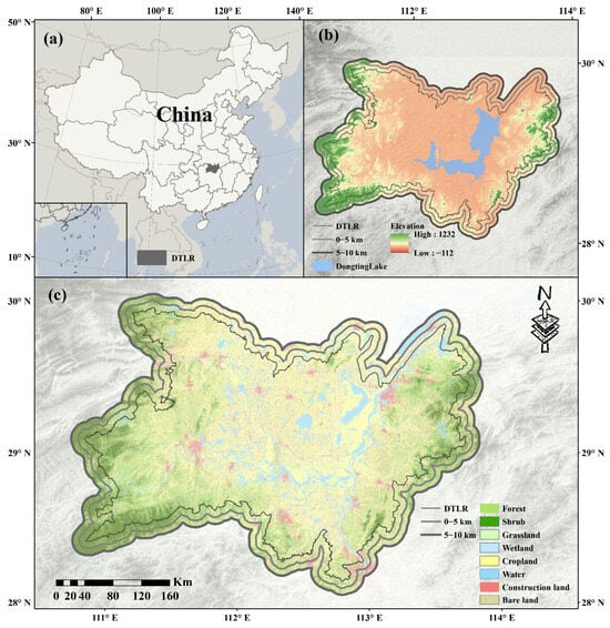
Figure 1. Maps of the Dongting Lake Region (DTLR) showing: (a) its geographical location; (b) a digital elevation model (DEM); and (c) the 5 km and 10 km buffering zones.

2.2. Data Resources

Our work chose the period between 2000 and 2020, a time marked by more significant land-use changes, to analyze the ECC and its dynamic evolution. The related data included in this study comprises five groups, i.e., land use and land change (LULC), digital elevation model (DEM), climate (temperature and precipitation), and socioeconomic and ecological environmental data. For LULC data, we employed the 30 m land-use distribution map of the Middle Reaches of the Yangtze River urban agglomeration, which was developed by Jiang et al. [21], utilizing the Continuous Change Detection and Classification (CCDC) method. The overall classification accuracy of the LULC data ranged from 89.0% to 90.15%, while the Kappa coefficient varied between 0.83 and 0.84, indicating a high level of agreement and reliable classification performance. A 90 m spatial resolution DEM of the DTLR was collected from the Geospaital Data Cloud (http://www.gscloud.cn). The DEM data can effectively represent the bottom topography of the DTLR for much of the period from 2000 to 2020. Other remote sensing data, like NDVI, NPP, and AOD during the period were processed within the Google Earth Engine (GEE). The 1 km monthly precipitation and temperature data and PM 2.5 data were sourced from the National Tibetan Plateau Data Center (https://data.tpdc.ac.cn/). Additionally, the LandScan dataset, provided by the Oak Ridge National Laboratory (ORNL), offers a comprehensive and high-resolution global population distribution dataset that serves as a valuable source. The 1 km grided revised real gross domestic product (GDP) was produced by Chen et al. [22] based on calibrated nighttime light data. Carbon emissions dataset was estimated based on the actual emission data from various energy sources from the province municipal statistics yearbook between 2000 and 2020.

All raster data preprocessing, spatial calculations, and the generation of buffer and influence zones were conducted using ArcGIS 10.8 and Python (version 3.12).

2.3. Research Methodology

The overall research framework integrating these components and methodologies is schematically represented in Figure 2. This study evaluated the ECC of DTLR and its buffer zone by integrating the DPSIRM model with a fine evaluation scale and multiple data sources (Table 1). Six dimensions encompassing 16 indicators were constructed to capture the fine-scale spatiotemporal dynamics of ECC over the past two decades. Indicator weights were determined through a combined Analytic Hierarchy Process (AHP) and entropy method. To examine temporal trends, Theil–Sen’s slope estimator and the Mann–Kendall (MK) test were employed, while geographically weighted regression (GWR) was used to analyze driving factors, disentangling the complex influences of internal and external ecosystem variables.

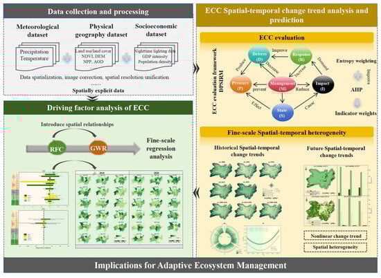
Figure 2. A comprehensive framework for evaluating ECC and analyzing its driving factors.

Table 1. Details of the data source.

Data Name	Data Description	Sources	Type	Resolution
Land-use and land change data	2000–2020 LULC dataset	Developed by Jiang, Liu, Liu, Peng, Liao, Wang and Gao [21]	tiff	30 m
NDVI	MODIS MYD13Q1	GEE (https://earthengine.google.com/)	tiff	250 m
Meteorological data	1 km monthly precipitation and temperature dataset for China	National Tibetan Plateau Scientific Data Center (https://data.tpdc.ac.cn/)	tiff	1000 m
DEM	DEM	Geospatial data cloud (http://www.gscloud.cn)	tiff	90 m
NPP	MODIS MOD17A3	GEE (https://earthengine.google.com/)	tiff	500 m
Population density	LandScan global population density data	U.S. Department of Energy, Oak Ridge National Laboratory (https://landscan.ornl.gov/)	tiff	1000 m
GDP intensity	GDP grid data	Developed by Chen, Gao, Cheng, Hou, Song, Liu and Liu [22] (https://doi.org/10.6084/m9.figshare.17004523.v1)	tiff	1000 m
Nighttime lighting data	A prolonged artificial nighttime light dataset (PANDA)	National Tibetan Plateau Scientific Data Center (https://data.tpdc.ac.cn/)	tiff	1000 m
AOD	MODIS/006/MCD19A2	GEE (https://earthengine.google.com/)	tiff	1000 m
PM2.5	PM2.5 grid data	National Tibetan Plateau Scientific Data Center (https://data.tpdc.ac.cn/)	tiff	1000 m
Carbon emissions	Carbon emissions accounting	Estimated on the basis of actual emission data from various energy sources from the Province Municipal Statistical Yearbook 2000–2020 and population data	tiff	1000 m
POI		Urban spatial quantitative research data platform (https://www.resdc.cn/DOI/)	vector
Administrative boundary		Geospatial data cloud (http://www.gscloud.cn/)	vector	1:100,000

2.3.1. ECC Evaluation

(1)

Construction of evaluation index system

The Pressure–State–Response (PSR) model, developed by Canadian statisticians David J. Rapport and Anthony Marcus Friend, conceptualizes interactions between human society and the environment through three components: pressures from human activities, resulting environmental states, and corresponding social response [23]. The DPSIRM model, an evolution of the PSR model, was developed by the European Environment Agency to enhance understanding of the broader socio-environmental system [24]. Based on the principles of objectivity, rationality, and accessibility in selecting index data, and considering the actual situation in DTLR, a total of 16 indicators were derived from six perspectives of ECC: Drivers, Pressures, States, Impacts, Responses, and Management.

These indicators were meticulously formulated based on the DPSIRM model, as delineated in Table 2. The Driving Forces component reflects the broader social, economic, and demographic factors that stimulate changes in the ECC of the DTLR. Population density, nightlight, and GDP were selected because they collectively represent the core socioeconomic gradients driving ecological change. Population density reflects human demand for land, water, and ecosystem services [25]; nighttime light serves as a spatial proxy for human activity intensity and economic development [26]; and GDP captures regional economic performance, which often accelerates resource consumption and land-use transformation [27]. These variables are widely recognized as foundational drivers in ECC and sustainability assessments. Pressure (P) represents the direct stresses generated by these Driving Forces—typically quantified through human activities that impose ecological burdens. AOD, PM 2.5, and carbon emission datasets were chosen as direct indicators of anthropogenic pressure. These datasets quantify the atmospheric pollution and carbon burden generated by industrial production, transportation, and energy consumption—activities that directly degrade ecological conditions and reduce the system’s carrying capacity. State (S) describes the biophysical condition of the DTLR ecosystem under the combined influence of Driving Forces and pressures. It is noteworthy to point out that the habitat quality index, an important indicator for characterizing the ability of an ecosystem to support species diversity and functionality, was calculated from the habitat quality module in InVEST [28,29]. Vegetation growth and cover describe primary productivity, ecosystem vigor, and the capacity of landscapes to regulate hydrological and biogeochemical processes. These three indicators together provide a robust description of ecological health. Impact (I) and Response (R) capture the ecological consequences and risks inherent in the adoption of adaptive or protective measures. Gross primary production (GPP) and the urban heat index (UHI, from InVEST) were selected to quantify the ecological impacts of human activities. GPP represents the system’s carbon sequestration and energy conversion capacity, while the UHI indicates climate-regulating capability and the extent of thermal stress. For the Response dimension, per capita green space and biodiversity conservation indices were chosen to capture societal and governmental efforts to alleviate ecological risks. Biodiversity conservation serves as a key indicator for biodiversity protection at both landscape and regional scales, as it is closely linked to habitat quality (HQ), net primary productivity (NPP), and landscape structure (LS) [30,31]. Landscape fragmentation (FR), separation (SE), and fractal dimension (FD) were calculated using the R software (version 4.2) “landscapemetrics” packages. To ensure comparability among indicators, min–max normalization was applied to HQ, NPP, and LS, after which the standardized values were integrated to construct a comprehensive biodiversity conservation index. Management (M) reflects the institutional capacity and governance mechanisms. Landscape connectivity reflects the effectiveness of ecological network planning; concentration degree of construction measures the intensity of built-up land management [32]; and urbanization rate reflects broader institutional decisions about land development. These indicators together characterize the institutional ability to regulate human–environment interactions and maintain ecological stability.

$$\mathrm{BI}=\sqrt[3]{\mathrm{H}\mathrm{Q}\times \mathrm{N}\mathrm{P}\mathrm{P}\times \mathrm{L}\mathrm{S}}$$

(1)

$$\mathrm{LS}=1-(0.5\times \mathrm{F}\mathrm{R}+0.3\times \mathrm{S}\mathrm{E}+0.2\times \mathrm{F}\mathrm{D})$$

(2)

Table 2. ECC indicator systems.

Target Layer	Guideline Layer	Indicator Layer	Unit	Feather
Ecological Carrying Capacity Indicators (A)	Drivers (B1)	Population density (C1)	Person/km2	−
		GDP (C2)	yuan	+
		Night light (C3)	-	+
	Pressure (B2)	AOD (C4)	-	−
		PM2.5 (C5)	µg/m3	−
		Carbon emissions (C6)	/mg/L	−
	State (B3)	Habitat quality index (C7)	-	+
		Vegetation growth status (C8)	-	+
		Vegetation cover(C9)	%	+
	Impact (B4)	GPP (C10)	kgC/m2/yr	+
		Urban heat mitigation index (C11)	-	+
	Response (B5)	Per capita green space (C12)	%	+
		Biodiversity conservation (C13)	-	+
	Management (B6)	Landscape connectivity (C14)	-	+
		Concentration degree of construction land (C15)	-	+
		Urbanization rate (C16)	%	−

(2)

Calculation of the evaluation indexes

The process of ascertaining the weights of six indicators may be classified into two distinct categories: subjective and objective weighting methods. Subjective weighting via Analytic Hierarchy Process (AHP) is derived by aggregating experts’ pairwise comparisons using the geometric mean and then calculating the principal eigenvector of the resulting matrix to produce a consensus priority scale [16], and entropy weighting, which provides an objective perspective by analyzing data variability [33]. It is founded on the principle that the degree of information an indicator provides is reflected in its variation; therefore, reduced variability corresponds to lower informational content and a lesser weight [34]. Entropy complements AHP by addressing its potential biases, resulting in a more robust and comprehensive weighting framework for decision making. In light of the intricacy and ambiguity inherent within the ECC system, this combined approach enables a more holistic and accurate assessment of the ECC. The formula for calculating the integrated weights using the two methods is provided in Equation (1). All indicator data were normalized and standardized using the min–max normalization method to ensure unit consistency. The detailed calculation results are presented in Supplementary Tables S1–S7. Based on expert judgments, a pairwise comparison matrix was constructed to represent the relative importance of each ECC evaluation indicator. Consistency tests were conducted for all hierarchical levels, and the resulting CR values were below 0.10, indicating acceptable matrix consistency. The AHP-derived weights for each level are reported in Tables S1–S7. Subsequently, the AHP–entropy combined weights for the 16 indicators were calculated, and the resulting integrated weights are presented in Table S8:

$${\mathrm{w}}_{\mathrm{i}}={\alpha {\mathrm{w}}_{\mathrm{i}}}^{\mathrm{A}\mathrm{H}\mathrm{P}}+(1-\alpha ){{\alpha \mathrm{w}}_{\mathrm{i}}}^{\mathrm{E}\mathrm{W}}$$

(3)

where α represents the proportion assigned to the AHP weights, which was set to 0.5 based on expert consensus, and ${{\mathrm{w}}_{\mathrm{i}}}^{\mathrm{A}\mathrm{H}\mathrm{P}}$, ${{\mathrm{w}}_{\mathrm{i}}}^{\mathrm{E}\mathrm{W}}$ denote the indicator weights derived from the AHP and entropy methods, respectively.

Following the previous research [18], the comprehensive index model of ECC was calculated based on the standardized index by using ArcGIS 10.8 and corresponding weight values, as follows:

$$\mathrm{E}\mathrm{C}\mathrm{C}={\displaystyle \frac{{\mathrm{S}}^{\mathrm{w}\mathrm{s}}\times {\mathrm{R}}^{\mathrm{w}\mathrm{t}}\times {\mathrm{M}}^{\mathrm{w}\mathrm{m}}}{{\mathrm{D}}^{\mathrm{w}\mathrm{d}}\times {\mathrm{P}}^{\mathrm{w}\mathrm{p}}\times {\mathrm{I}}^{\mathrm{w}\mathrm{i}}}}$$

(4)

where ECC stands for the Ecological Carrying Capacity. ${\mathrm{D}}^{\mathrm{w}\mathrm{d}}$, ${\mathrm{P}}^{\mathrm{w}\mathrm{p}}$, ${\mathrm{I}}^{\mathrm{w}\mathrm{i}}$, ${\mathrm{S}}^{\mathrm{w}\mathrm{s}}$, ${\mathrm{R}}^{\mathrm{w}\mathrm{t}}$, and ${\mathrm{M}}^{\mathrm{w}\mathrm{m}}$ represent the weight value of Driving Forces, Pressure, Impact, State, Response, and Management subsystem, respectively.

The ECC index was calculated using the established formulas and subsequently classified into five categories—very low, low, medium, high, and very high—using the Natural Breaks (Jenks) method. This classification approach was selected because it identifies the most meaningful class boundaries based on the intrinsic data distribution, minimizing within-class variance while maximizing between-class differences, thereby producing groups of ECC values that are internally coherent and analytically robust.

2.3.2. ECC Trend Analysis and Prediction

(1)

Trend analysis of ECC

Theil–Sen’s slope and the Mann–Kendall (MK) test were performed to depict the statistical significance of ECC trends from 2000 to 2020. The Theil–Sen approach is a nonparametric method that calculates the slope between all pairs of data points, ranks these slopes in ascending order, and identifies the median slope as the overall trend [35].

$$\beta =\mathrm{Median} ({\displaystyle \frac{{\mathrm{X}}_{\mathrm{j}}-{\mathrm{X}}_{\mathrm{i}}}{\mathrm{j}-\mathrm{i}}}),\forall \mathrm{j}>\mathrm{I}$$

(5)

where β is indicative of the evolving trend in the data, with positive and negative values signifying the direction of the trend; when β exceeds 0, the change in the data shows an upward trend; conversely, while β is less than 0, the trend demonstrates a downward trajectory.

The Mann–Kendall test is a nonparametric statistical method employed for the identification of trends in data that are not required to conform to a particular distribution. The test is straightforward to compute, making it widely applicable for analyzing time series data.

$$\mathrm{S}={\sum }_{\mathrm{i}=1}^{\mathrm{n}-1}{\sum }_{\mathrm{j}=\mathrm{i}+1}^{\mathrm{n}}\mathrm{S}\mathrm{i}\mathrm{g}\mathrm{n} ({\mathrm{T}}_{\mathrm{j}}-{\mathrm{T}}_{\mathrm{i}})$$

(6)

$$\mathrm{S}\mathrm{i}\mathrm{g}\mathrm{n} ({\mathrm{T}}_{\mathrm{j}}-{\mathrm{T}}_{\mathrm{i}})=\left\{\begin{array}{cc}1,\hspace{1em}\hfill & {\mathrm{T}}_{\mathrm{j}}-{\mathrm{T}}_{\mathrm{i}}>0\hfill \\ 0,\hspace{1em}\hfill & {\mathrm{T}}_{\mathrm{j}}-{\mathrm{T}}_{\mathrm{i}}=0\hfill \\ -1,\hspace{1em}\hfill & {\mathrm{T}}_{\mathrm{j}}-{\mathrm{T}}_{\mathrm{i}}<0\hfill \end{array}\right.$$

(7)

where n is the number of sequence samples, and ${\mathrm{T}}_{\mathrm{j}}$ and ${\mathrm{T}}_{\mathrm{i}}$ are the ECC values of years j and i, respectively. The results indicate that, when n ≥ 10, S approximately follows a normal distribution. By standardizing S, the test statistic Z is derived, with standardization performed using the following formula:

$$\mathrm{Z}=\left\{\begin{array}{cc}{\displaystyle \frac{\mathrm{S}+1}{\sqrt{\mathrm{Var}\left(\mathrm{S}\right)}}},\hspace{1em}\hfill & \mathrm{S} > 0\\ 0,\hspace{1em}\hfill & \mathrm{S} = 0\\ {\displaystyle \frac{\mathrm{S}-1}{\sqrt{\mathrm{Var}\left(\mathrm{S}\right)}}},\hspace{1em}\hfill & \mathrm{S} > 0\end{array}\right.$$

(8)

When using a two-tailed test with a significance level of α = 0.05, the critical value from the normal distribution table is Z_0.05 = ±1.96. When |Z| is less than or equal to |Z_0.05|, the null hypothesis (H₀) is accepted, indicating no significant trend in the time series. Conversely, if |Z| is greater than |Z_0.05|, H₀ is rejected, showing a clear increasing or decreasing trend in the data. In order to better describe the change trend of ECC, we divided the S into 6 classes in our research: severe degradation, slight degradation, no obvious degradation, slight improvement, significant improvement, and no obvious improvement (Table 3).

Table 3. The classification of the ECC changes trend.

Trend	Sen (β)	MK Test
significant improvement	β > 0	p < 0.01
slight improvement	β > 0	0.01 ≤ p < 0.05
no obvious improvement	β > 0	p ≥ 0.05
no obvious degradation	β < 0	p ≥ 0.05
slight degradation	β < 0	p < 0.01
severe degradation	β < 0	p < 0.01

(2)

Coefficient of variation

Coefficient of variation (CV) is commonly used to reflect the discrete degree and the volatility of the time series data. It is calculated by

$$\mathrm{C}={\displaystyle \frac{\sqrt{\frac{{\sum }_{\mathrm{i}=1}^{\mathrm{n}}({\mathrm{E}\mathrm{C}\mathrm{C}}_{\mathrm{i}}-\overline{\mathrm{E}\mathrm{C}\mathrm{C}})}{\mathrm{n}-1}}}{\overline{\mathrm{E}\mathrm{C}\mathrm{C}}}}$$

(9)

where C is the CV of ECC, referring to the coefficient of variation in the ECC of each pixel in 2000–2020; ECC_i represents the ECC of the year i and $\overline{\mathrm{E}\mathrm{C}\mathrm{C}}$ is the mean ECC value. A larger CV signifies larger data fluctuation in the ECC time series, while a smaller CV denotes a more stable ECC time series.

(3)

Hurst exponent

The Hurst exponent, initially proposed by Hurst [36], is a statistical tool used to evaluate the sustainability or long-term memory of time series data. It has been extensively applied across disciplines, including hydrology, climatology, geology, and economics. In our study, we used the Hurst exponent to detect ECC variations. The primary calculation procedures are as follows [37]:

To define the time series, i = 1, 2, 3… j.

To define the mean sequence of the time series

$${\overline{\mathrm{E}\mathrm{C}\mathrm{C}}}_{\mathrm{j}}={\displaystyle \frac{1}{\mathrm{j}}}{\sum }_{\mathrm{i}=1}^{\mathrm{j}}{\mathrm{E}\mathrm{C}\mathrm{C}}_{\mathrm{i}}$$

(10)

To calculate the accumulated deviation

$${\mathrm{X}}_{\mathrm{i},\mathrm{j}}={\sum }_{\mathrm{i}=1}^{\mathrm{i}}({\mathrm{E}\mathrm{C}\mathrm{C}}_{\mathrm{i}}-{\overline{\mathrm{E}\mathrm{C}\mathrm{C}}}_{\mathrm{j}}), 1\le \mathrm{i}\le \mathrm{j}$$

(11)

To create the range sequence

$${\mathrm{R}}_{\mathrm{j}}=\underset{1\le \mathrm{i}\le \mathrm{j}}{\mathrm{m}\mathrm{a}\mathrm{x}} {\mathrm{X}}_{\mathrm{i},\mathrm{j}}-\underset{1\le \mathrm{i}\le \mathrm{j}}{\mathrm{m}\mathrm{i}\mathrm{n}} {\mathrm{X}}_{\mathrm{i},\mathrm{j}}$$

(12)

To create the standard deviation sequence

$${\mathrm{S}}_{\mathrm{j}}={\left[{\displaystyle \frac{1}{\mathrm{j}}}{\sum }_{\mathrm{i}=1}^{\mathrm{j}}({\mathrm{E}\mathrm{C}\mathrm{C}}_{\mathrm{i}}-{\mathrm{E}\mathrm{C}\mathrm{C}}_{\mathrm{j}}{)}^2\right]}^{{\displaystyle \frac{1}{2}}}$$

(13)

To calculate the Hurst exponent

$${(\mathrm{R}/\mathrm{S})}_{\mathrm{j}}=\mathrm{C}{\mathrm{j}}^{\mathrm{H}}$$

(14)

H is the Hurst exponent, which can be expanded from 0 to 1. If 0 < H < 0.5, it indicates that the ECC time series is not persistent, and future changes are inversely correlated with the past; if 0.5 < H < 1, it indicates that the changes in the ECC time series have persistence, and the future trend is consistent with the past trend; and if H = 0.5, it indicates that the ECC time series is a stochastic series without sustainability, and the future trend is not correlated with the past change trend.

2.3.3. Driving Force Analysis

Geographically weighted regression (GWR) is a local form of regression analysis that accounts for spatial heterogeneity in data [38,39]. Unlike traditional multivariate linear models, which assume that the relationships between variables remain constant, GWR explicitly accommodates spatial non-stationarity by estimating local regression coefficients for each observation or location. GWR often leads to a better fit than traditional global regression models and can detect the spatial variations in the relationship between independent and dependent variables [19].

In this study, we first employed ordinary least squares (OLS) regression to establish a global assessment of the relationships between ECC and its driving factors [40], while also evaluating the overall model fit and residual spatial autocorrelation. Moran’s I was used to test for spatial autocorrelation in the OLS residuals, aiding in the detection of potential spatial heterogeneity [41]. Given that the residuals frequently displayed significant spatial dependence, we subsequently applied geographically weighted regression (GWR) to capture localized variations in these relationships. The GWR model utilized a Gaussian kernel function to define spatial weights, and an adaptive bandwidth was automatically selected by minimizing the corrected Akaike Information Criterion (AICc) [42]. This approach ensures that nearby observations are appropriately weighted at each location, enabling the derived local regression coefficients to accurately represent the spatially varying influence of each driving factor [40].

By using GWR, we took the ECC value in 2010 and 2020 as the dependent variable and used five types of factors, like natural environmental factors, geographical zoning factors, road traffic factors, socioeconomic factors, and landuse and land cover change factors as independent variables (Table 4). The regression coefficients of each factor were visualized using ArcGIS, and the influence of each factor on the ECC was analyzed. The GWR formula is as follows:

$${\mathrm{y}}_{\mathrm{i}}={\beta }_0\left({\mathrm{u}}_{\mathrm{i}},{\mathrm{v}}_{\mathrm{i}}\right)+{\sum }_{\mathrm{i}=1}^{\mathrm{k}}{\beta }_{\mathrm{j}}\left({\mathrm{u}}_{\mathrm{i}},{\mathrm{v}}_{\mathrm{i}}\right){\mathrm{x}}_{\mathrm{j}\mathrm{i}}+{\mathrm{e}}_{\mathrm{i}}$$

(15)

where $y_i$ denotes the ECC, ${\beta }_0\left({\mathrm{u}}_{\mathrm{i}},{\mathrm{v}}_{\mathrm{i}}\right)$ is the intercept at the location i, k is the total number of spatial units, ${\beta }_{\mathrm{j}}\left({\mathrm{u}}_{\mathrm{i}},{\mathrm{v}}_{\mathrm{i}}\right)$ is the local estimated regression coefficient of ${\mathrm{x}}_{\mathrm{j}\mathrm{i}}$, ${\mathrm{x}}_{\mathrm{j}\mathrm{i}}$ is the value of the independent variable j, $\left({\mathrm{u}}_{\mathrm{i}},{\mathrm{v}}_{\mathrm{i}}\right)$ is the space coordinate of sample i, and ${\mathrm{e}}_{\mathrm{i}}$ is the random error. All variables were standardized using the Z-score method before using the GWR model [43].

Table 4. Five types of exploratory (independent) variables.

Types of Factors	Driving Forces	ID	Unit
Natural environmental factors	DEM	X1	m
	Slope	X2	°
	Precipitation	X3	mm
	Temperature	X4	°
Geographical zoning factors	Distance to the center of Greenheart	X5	m
	Distance to the center of Yueyang	X6	m
	Distance to the center of Changsha	X7	m
	Distance to the center of Changde	X8	m
	Distance to the center of Yiyang	X9	m
Road traffic factors	Distance to the highway	X10	m
	Distance to the national highway	X11	m
	Distance to the railroad	X12	m
Socioeconomic factors	Density of public service equipment	X13	/km2
	Density of commercial service equipment	X14	/km2
	Density of leisure service equipment	X15	/km2
Land-use and land cover change factors	New forest area	X16	km2
	New impervious area	X17	km2

3. Results

3.1. Weighting Values Between Evaluation Indicators

The AHP–entropy weighting approach was employed to quantify the relative importance of 13 indicators, as derived from the data in Table 2. The weight of ECC is the aggregate of the indicators’ weights ascribed to this subsystem. As presented in Table 5, hierarchical ranking based on subsystem significance reveals the following order: Pressure subsystem (P: 0.2542) > Management subsystem (M: 0.2323) > Driver subsystem (D: 0.2112) > State subsystem (S: 0.1111) > Influence subsystem (I: 0.1019) > Response subsystem (R: 0.0894). This hierarchy indicates that Pressure and Management factors play dominant roles in shaping the whole system, while the other subsystems contribute in supportive or reactive capacities.

Table 5. The weights of the ECC indicators were derived through an integrated approach that combines the Analytic Hierarchy Process (AHP) with the entropy weighting (EW) method.

Target Layer	Guideline Layer	Indicator Layer	Unit	Weight	Total Weight	Feather
Ecological Carrying Capacity Indicators	Drivers	Population density	Person/km2	0.0716	0.2112	−
		GDP	yuan	0.0711		+
		Night light	-	0.0685		+
	Pressure	AOD	-	0.1069	0.2542	−
		PM2.5		0.0982		−
		Carbon emissions	/mg/L	0.0491		−
	State	Habitat quality index	-	0.0481	0.1111	+
		Vegetation growth status		0.0261		+
		Vegetation cover	%	0.0368		+
	Impact	GPP	kgC/m2/yr	0.0519	0.1019	+
		Urban heat mitigation index	-	0.05		+
	Response	Per capita green space	%	0.0324	0.0894	+
		Biodiversity conservation		0.057		+
	Management	Landscape connectivity		0.0307	0.2323	+
		Concentration degree of construction land		0.1183		+
		Urbanization rate	%	0.0832		−

3.2. Changes in ECC Subsystem Indexes

To illustrate the spatial-temporal heterogeneity of ECC in DTLR, this work summarizes the evaluation results of six subsystems from 2000 to 2020 and compares the evolving trends of ECC in three areas, including the DTLR, the 0–5 km buffer zone, and the 5–10 km buffer zone (Figure 3). The change patterns of these six subsystem indices were analyzed sequentially to identify key dynamics over time.

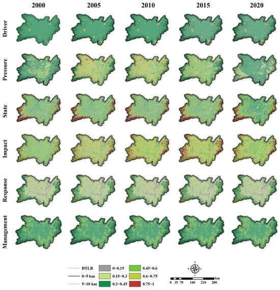
Figure 3. Spatial heterogeneity of criteria layer of ECC from 2000 to 2020.

As illustrated in Figure 4, both the Driver and Response subsystems exhibited an increasing trend from 2000 to 2020. More precisely, the Driver index increased from 0.350 to 0.367 in the DTLR, from 0.350 to 0.371 in the 0–5 km buffer zone, and from 0.356 to 0.375 in the 5–10 km buffer zone. Similarly, the Response index increased from 0.203 to 0.211 in the DTLR, from 0.286 to 0.305 in the 0–5 km buffer zone, and from 0.297 to 0.320 in the 5–10 km buffer zone, respectively. Spatially, these two subsystems indicate minimal variation across the region during the study period (Figure 3). Analysis of the trends in the Pressure, State, and Impact indices revealed two distinct stages (Figure 4b–d). In the first stage (2000–2010), both the Pressure and Impact indices in the DTLR exhibited an upward trend, rising from 0.390 to 0.661 and from 0.549 to 0.686, respectively. Among the three regions, the DTLR exhibited the highest value, followed by the 0–5 km buffer zone and the 5–10 km buffer zone, indicating a gradient of decreasing values with increasing distance from the core area. In contrast, the Impact and State index showed an opposite trend, with the 0–5 km and 5–10 km buffer zones showing comparatively higher values than the DTLR. In the second stage (2010–2020), the Pressure index revealed a significant downward trend, decreasing at an average annual rate of 49.15% across the three regions. The Impact and State index showed more moderate decreases, averaging 5.37% and 7.57%, respectively. Spatially, the Pressure subsystem exhibited higher values in the central areas, with decreasing intensity toward the periphery (Figure 3). The overall trend of the Management subsystem followed a U-shaped curve during 2000–2020 (Figure 4f). Its lowest values occurred in 2003 (0.409) in the 5–10 km zone, in 2009 (0.414) in the 0–5 km zone, and in 2011 (0.416) within the DTLR. The spatial distribution of the Management subsystem shows a diminishing gradient from the periphery to the core area of the study area (Figure 3). Areas with high values were mainly dispersed across rural and suburban regions, while low-value areas were primarily clustered in the urban core.

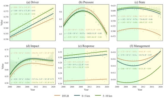
Figure 4. Comparison of the value of six subsystems in DTLR with 0–5 km buffer and 5–10 km buffer.

3.3. Spatial-Temporal Heterogeneity of ECC

This study divided the ECC index into five levels, very low, low, medium, high, and very high, by using the Natural Breaks Class method. Figure 5 depicts the categorization properties of the ECC across several time scales in the study area.

Figure 5. Spatial distribution and temporal evolution of ECC (2000–2020). (a–e) illustrate the spatial patterns of ECC for the years 2000, 2005, 2010, 2015, and 2020. (f–h) depict the net change in ECC across three-time intervals: 2000–2010, 2010–2020, and the full study period of 2000–2020. (i) The temporal evolution of area proportions for different ECC intensity levels. (j) The ECC trajectory for the DTLR, the 0–5 km buffer, and the 0–10 km buffer zones.

In general, the results show that ECC presented uneven spatial distributions from 2000 to 2020. Throughout the study period, ECC consistently exhibited higher values in peripheral areas compared to the central core. This suggests that the rural area of study possesses a greater resilience and capacity, likely attributed to its favorable natural conditions. Comparatively, ECC showed distinct spatiotemporal dynamics across the DTLR, the 0–5 km buffer, and the 5–10 km buffer zones between 2000 and 2020 (Figure 5i,j). During the study period, the temporal patterns of ECC change among the three subregions were well synchronized, revealing a U-shaped curve (Figure 5j). Specifically, the ECC of the three subregions decreased from 2000 to 2010, with the average ECC value reaching 0.416 (DTLR), 0.447 (0–5 km buffer), and 0.449 (5–10 km buffer), respectively. However, the ECC in most areas increased from 2010 to 2020, with the average value accounting to 0.436, 0.467, and 0.469, respectively (Figure 5j). In addition, the ECC in the 5–10 km buffer consistently recorded the highest value throughout the year, followed by the 0–5 km buffer and DTLR. The classification statistics for ECC at multiple time scales in the three subregions are shown in Figure 5h. In 2000, areas with very high ECC covered 13.34% of the DTLR, 39.73% of the 0–5 km buffer, and 43.02% of the 5–10 km buffer. By 2020, these proportions had steadily increased to 40.34%, 63.78%, and 57.72%, respectively. From 2000 to 2010, the average area percentages of both high and low ECC levels in all three subregions experienced a decline, from 36.91% and 6.11% in 2000 to 29.85% and 2.87% in 2010, before rising again in the following years. In contrast, the very low ECC initially fluctuated upward until 2011, after which it began to decline in the DTLR; meanwhile, in the 0–5 m and 0–10 m buffer zones, the very low ECC showed an N-shaped fluctuation. The percentage of medium ECC remained relatively unchanged across three subregions during the study period, fluctuating from 30.73% to 40.05% in the DTLR, 16.44% to 25.62% in the 0–5 km buffer zone, and 16.18% to 8.37% in the 5–10 km buffer zone, respectively.

3.4. Analysis of ECC Change Trend

The trend analysis based on time series data offers valuable insights into the historical fluctuations and potential future trajectories of ECC. Figure 6 presents the results of the Sen’s slope value and the MK significance test. The area exhibiting no significant increase during 2000–2020 accounted for the largest proportion, surpassing 90%, followed by areas with a very significant decrease, which constituted approximately 3% in three subregions, predominantly located in the interior of Dongting Lake. Notably, the significance and pattern of ECC changes varied considerably across different stages. During 2000–2010, the largest proportion in all the three subregions experienced a very significant decrease, whereas in the subsequent 2010–2020 period, the largest proportion showed no significant increase.

Figure 6. Spatiotemporal trend of ECC in DTLR, 0–5 km buffer, and 5–10 km buffer during 2000–2020 period. (a1–a3) Theil–Sen trend of ECC; (b1–b3) MK trend of ECC; and (c1–c3) the percentage of significance of ECC change during the period.

The coefficient of variation (CV) is a useful metric for characterizing the degree of dispersion and volatility of ECC within a time series. During 2000–2020, the CV in the DTLR, the 0–5 km buffer zone, and the 5–10 km buffer zone ranged from 0.01 to 0.29, 0.02 to 0.23, and 0 to 0.24, respectively (Figure 7a). The spatial stability of ECC changes in our study area was characterized by a generally uniform distribution, with relative stability in rivers and mountainous regions and more fluctuations in urban areas. Specifically, an increasing proportion of areas exhibited low volatility moving from the DTLR to the outer regions, with percentages of 8.92%, 20.00%, and 25.52%, respectively. The proportion of areas with relatively low volatility decreased in a descending order from the DTLR, 0–5 km buffer zone, and 5–10 km buffer zone, with values of 90.12%, 79.38%, and 73.63%, respectively.

Figure 7. Spatial distribution of sustainability and the future trend of ECC in three subregions.

With regard to the projected future trend (Figure 7b), ECC changes were classified into four classes based on the Hurst exponent, namely, anti-persistent increase, persistent increase, anti-persistent decrease, and persistent decrease. The results indicated that the anti-persistent increase (indicating a shift from improvement to degradation) represented approximately 33.73%, 31.84%, and 32.82% of the DTLR, 0–5 km buffer zone, and 5–10 km buffer zone, respectively (Figure 7b2). This trend was mainly distributed in the central and eastern parts of the study area, especially in the western part of Dongting Lake (Figure 7b1). The anti-persistent decrease (indicating a shift from degradation to improvement), which represented the largest proportion, accounted for approximately 62.55%, 65.10%, and 57.52% in the DTLR, 0–5 km buffer zone, and 5–10 km buffer zone, respectively. This trend was distributed in the western part of the study area. The proportion of areas with a persistent increase amounted to 2.15%, 1.28%, and 1.34%, respectively, mainly distributed in the interior of Dongting Lake.

In summary, the future trend of ECC change in DTLR and its surrounding areas is predominantly characterized by improvement, suggesting that the region is likely to experience enhanced resilience and sustainability in the years ahead.

3.5. Driving Factor Analysis of the Ecological Carrying Capacity

The study compared evaluation parameters between OLS and GWR models, as shown in Table S8. For both 2010 and 2020, OLS residuals showed significant spatial autocorrelation (Moran’s I ≈ 0.37–0.38, p = 0.001), with relatively low R² (≈0.82–0.83). In contrast, GWR residuals were close to zero in Moran’s I (p > 0.25), with higher R² (0.95–0.96), indicating better fit and accounting for spatial heterogeneity. Therefore, GWR was employed to further analyze the spatial heterogeneity of ECC driving factors.

The results showed that the maximum adjusted R² of the resulting conclusion was 0.95 in 2010 and 0.96 in 2020, suggesting no issues with multicollinearity. As shown in Figure 8 and Figure 9, the effects of different variables on ECC changed significantly from 2010 to 2020. It was evident that the estimated coefficients for variables such as Distance to the center of Greenheart (X5), Distance to the national highway (X11), density of public service equipment (X13), density of commercial service equipment (X14), and new impervious area (X17) showed a negative impact on ECC in 2010. Among these, X5 had the most substantial effect on ECC (−1.72), with the regression coefficient gradually decreasing from west to east (Figure 9e1). All natural environmental factors (X1–X4) consistently contributed positively to ECC, indicating their critical role in enhancing regional sustainability. In terms of spatial distribution, the regression coefficients of these factors revealed consistent spatial patterns between 2010 and 2020. The geographical distance of DTLR from the four major cities influenced ECC positively in 2010, possibly through policy intervention that prioritized environmental protection in more distant areas. The positive correlations between the density of leisure service equipment (X15) and new forest area (X16) and ECC underscore the effectiveness of green cover in promoting ecological sustainability. Over time, the influence of the natural environmental factors, the geographical distance to the three cities, X15, and X16 on ECC gradually expanded. Meanwhile, the impact of road traffic factors and socioeconomic factors on ECC demonstrated a gradual increase in negative influence, with regression coefficients for variables X9, X12, X13, and X14 changing from 0.09, −0.08, and −0.33 in 2010 to −0.11, −0.48, and −0.33 in 2020, respectively.

Figure 8. (a,b) Influence of driving factors on ECC from 2010 to 2020. Background shading distinguishes the study years, with light orange indicating 2010 and light green indicating 2020. Asterisks denote statistical significance: ** p < 0.01 and *** p < 0.001.

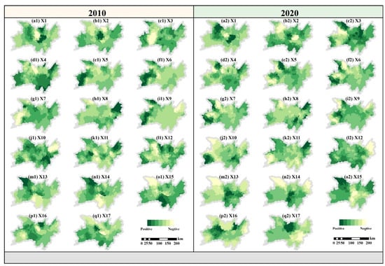
Figure 9. GWR coefficients of 17 Driving Forces in 2000 and 2020.

4. Discussion

4.1. Spatiotemporal Evolution of ECC and Its Link to Urbanization

Our analysis reveals a distinct U-shaped trajectory in the Ecological Carrying Capacity (ECC) of the Dongting Lake Region (DTLR) from 2000 to 2020, a pattern intrinsically linked to the region’s urbanization stages and policy evolution (Figure 5). At the beginning of the 21st century, China underwent tremendous structural changes in its economy and financial system, reshaping the global economic landscape [44]. During this time, environmental policies, such as the “Returning Farmland to Lakes” initiative, were implemented; however, their scope and enforcement proved insufficient to fully address the widespread ecological pressures stemming from agriculture and urbanization. The observed decline in ECC during this decade can be directly attributed to the imbalance between developmental pressure and conservation efforts (Figure 5). A decisive reversal began post-2010, with the ECC recovery rate surpassing the previous rate of decline (Figure 5). At the national level, China’s environmental policies faced a crucial turning point, and environmental protection began to gain prominence as a key policy objective. This upturn aligns with a national strategic pivot that elevated environmental protection, marked by the 12th Five-Year Plan (2011) and the introduction of the “Ecological Red Line” policy. At the regional level, the State Council officially approved the Dongting Lake ecological economic zone in 2014, marking a milestone for the coordinated management of the lake and its surrounding areas. The plans were designed to address the ecological degradation and challenges facing the DTLR. As a result, the improvement of ECC in the DTLR has been bolstered by these measures, which is consistent with the research by Su et al. [45], indicating that policy interventions lead to more than a 50% reduction in environmental pollution. Additionally, the transition from a passive response to active and comprehensive management has greatly enhanced the effectiveness of ecological governance, playing a crucial role in the region’s ecological recovery and the improvement of ECC.

Spatially, the ECC in the buffer zones is significantly higher than that in the DTLR, as illustrated in Figure 4. This discrepancy can primarily be attributed to the heterogeneous impacts of human activities (e.g., overfishing and deforestation), with urbanization and land-use changes in the core area contributing to a degraded ECC [46]. The buffer zone often encompasses or adjoins nature reserves, thereby shielding it from the full impact of urbanization [47,48]. This spatial disparity underscores the need for targeted interventions aimed at strengthening ecological governance, balancing development and conservation efforts, and ensuring the long-term sustainability of both the core area and the buffer zones of DTLR.

4.2. Driving Mechanisms of ECC

To elucidate the drivers of the Ecological Carrying Capacity (ECC), we employed a geographically weighted regression (GWR) model incorporating environmental, geographical, socioeconomic, and land-use factors. Our analysis reveals a complex interplay of influences, with several key mechanisms emerging. Among all factors, the most significant negative driver was the distance from the “Greenheart”, highlighting the critical role of proximity to intact ecosystems for maintaining ECC. Areas located farther from these ecological hubs tend to experience higher habitat fragmentation, concentrated pollution, and less efficient ecosystem services. Existing research highlights that Greenheart acts as a buffer zone between human-dominated landscapes and natural habitats, playing an essential role in ecological health [49]. ECC is also negatively impacted by the impervious surface area and the density of infrastructure (Figure 8). Urbanized areas, with their dense infrastructure, often lead to the occupation or destruction of wetlands, forest lands, and other vital ecosystems [50]. These land-use changes, accompanied by resource extraction and energy consumption, may aggravate the contradiction between economic development and ecological protection; this, in turn, further challenges ecosystem integrity and pushes ECC toward overloaded states. In our study, we found that the proximity to highways and railways might correlate with higher ECC. Typically, we associate highways with negative impacts on the ecosystem due to habitat fragmentation; however, in certain circumstances, they may serve as linear ecological corridors or connectivity routes between patches of forests or wetlands [51,52]. In such cases, highways and railways can facilitate species movement, promote genetic exchange between populations, and help maintain ecosystem functions across fractured landscapes. Moreover, when located near areas with well-designed ecological management measures—such as green belts, wildlife underpasses, and designated ecological corridors—these transportation routes can actually improve ecosystem connectivity and, consequently, enhance ECC.

Conversely, increasing forest cover and promoting leisure equipment (such as parks and recreational facilities) are both essential strategies for enhancing ECC (Figure 8). The forest provides numerous ecosystem services, such as carbon sequestration, water purification, and climate regulation [53], that directly benefit the ECC of a region. Similarly, the presence of leisure equipment enhances sustainable human–environment interactions and helps create a sense of environmental stewardship, which, in turn, supports a higher ECC. Changes in ECC are often caused by variations in natural factors (e.g., DEM, slope, temperature, and precipitation). In the DTLR, mountainous regions surrounding the lake are higher in elevation, typically with limited human settlement and diminished agriculture pressures, potentially creating a geographical divide from the low ECC region.

These findings collectively underscore “green infrastructure” as a foundational strategy for enhancing urban ecological resilience [54]. An interconnected network of green spaces, ranging from core forests to recreational corridors, can effectively mitigate the adverse impacts of urban sprawl. For urban planners, this translates to a strategic imperative: prioritizing the preservation and functional connection of natural areas is paramount for sustaining ECC in developing regions [55].

4.3. Policy Implications

As a pivotal ecological asset in the Yangtze River Basin, the Dongting Lake Region (DTLR) necessitates governance strategies informed by the precise spatial diagnostics of its Ecological Carrying Capacity (ECC). Achieving this necessitates measuring current ECC levels, analyzing their spatiotemporal dynamics, and identifying the key driving factors underlying these changes. The ensuing policy implications are derived from the findings of this study:

First, strategic public investment must be scaled to address the governance–pressures mismatch. The post-2011 ECC recovery demonstrates policy efficacy, yet the slower growth of management capacity compared to mounting environmental pressures reveals a critical vulnerability. This phenomenon suggests that the governance mechanisms in place—such as policies, enforcement, and institutional frameworks—are not evolving or scaling up rapidly enough to effectively address the mounting environmental pressures. We recommend a substantial increase in directed fiscal transfers for conservation projects, coupled with capacity-building programs for local governments. The deployment of advanced, real-time monitoring networks is essential to provide actionable data, enabling preemptive and more effective environmental management.

Second, spatial planning must prioritize the establishment of a functional “ecological network”, which includes buffer zones surrounding protected areas, biological corridors, and ecological stepping stones. Our findings reveal that ECC is significantly higher within 0–10 km buffer zones, highlighting their strategic importance. Policy should therefore explicitly delineate and safeguard these zones surrounding core wetlands and forests, integrating them with ecological corridors and stepping stones. Such a networked green infrastructure has been proven to mitigate land-use disturbances and industrial encroachment, thereby enhancing regional ecological resilience.

Thirdly, a fundamental paradigm shift from GDP-centric to ecology-led development is imperative. At present, the coordination of socioeconomic development and environmental protection is indeed one of the most pressing challenges faced by local government. The negative impacts associated with expanding impervious surface and dense infrastructure underscore the need to move beyond conventional urban sprawl models. Enhancing ECC in the DTLR demands a definitive break from the “GDP-centric” development paradigm. This entails the adoption of a new development framework that establishes binding ecological thresholds for all spatial and macroeconomic policy, prioritizing green infrastructure and ensuring that resource use is decoupled from economic growth.

4.4. Limitations and Outlook

While our study provides a spatially explicit assessment of ECC, several limitations warrant consideration and guide future research directions. First, although the selection of ECC indicators was based on the DPSIRM framework, it was constrained by data availability and inherently involves a degree of expert judgment. Future efforts should prioritize the development of a more standardized, universally applicable indicator system to enhance objectivity and cross-regional comparability. Second, methodological simplifications are inherent to model-based approaches. The structuring of the DPSIRM framework and the assumptions of the GWR model, while effective for capturing broad spatial patterns, may not fully represent the non-linear feedback and complex interdependencies within the social–ecological system. Subsequent research could integrate system dynamics models or agent-based modeling to better simulate these complex interactions. Third, the temporal scope and resolution of our data may not fully capture interannual climatic variability or abrupt ecological shifts. Future studies would benefit from incorporating higher-frequency time series data and validating the transferability of this assessment framework to other ecologically sensitive regions with distinct socioeconomic contexts. Addressing these limitations will be crucial to advancing ECC science. By incorporating a broader suite of dynamic variables and refining modeling techniques, future research can enhance the robustness, predictive power, and practical utility of ECC assessments for guiding sustainable ecosystem management.

5. Conclusions

This study examined the spatiotemporal dynamics and drivers of Ecological Carrying Capacity (ECC) in the Dongting Lake Region (DTLR) from 2000 to 2020. Our analysis reveals a distinct U-shaped trajectory in ECC, strongly correlated with urbanization phases and key environmental policies. This overall trend reflects divergent subsystem pathways: while the Management index improved consistently, the Pressure, State, and Impact indices followed an inverted U-shaped curve, peaking mid-period before declining. Future projections suggest that ECC in DTLR and its surrounding areas will continue to improve, indicating increased resilience and sustainability in the coming years. Key drivers identified include the negative impact of impervious surfaces and infrastructure density and the positive contributions of forest cover and accessible leisure facilities.

We proposed three management options to help increase ECC in the DTLR: (1) Implement an optimized green development strategy that prioritizes and scales strategic public investment in environmental conservation; (2) formulate a functional “ecological network” by establishing buffer zones, biological corridors, and ecological stepping stones to structurally enhance ECC connectivity; and (3) shift from a “GDP-centric” to an “ecology-led” development paradigm, embedding binding ecological thresholds as the foundation for all spatial planning and macroeconomic policy.

References

- Chen, Y.; Tian, W.; Zhou, Q.; Shi, T. Spatiotemporal and driving forces of Ecological Carrying Capacity for high-quality development of 286 cities in China. J. Clean. Prod. 2021, 293, 126186. [Google Scholar] [CrossRef]
- Xiong, S.; Yang, F. Ecological resilience in water-land transition zones: A case study of the Dongting Lake region, China. Ecol. Indic. 2024, 166, 112284. [Google Scholar] [CrossRef]
- Tomscha, S.; Jackson, B.; Benavidez, R.; de Róiste, M.; Hartley, S.; Deslippe, J. A multiscale perspective on how much wetland restoration is needed to achieve targets for ecosystem services. Ecosyst. Serv. 2023, 61, 101527. [Google Scholar] [CrossRef]
- Yang, L.; Wang, L.; Yu, D.; Yao, R.; He, Q.; Wang, S.; Wang, L. Four decades of wetland changes in Dongting Lake using Landsat observations during 1978–2018. J. Hydrol. 2020, 587, 124954. [Google Scholar] [CrossRef]
- Yu, Y.; Mei, X.; Dai, Z.; Gao, J.; Li, J.; Wang, J.; Lou, Y. Hydromorphological processes of Dongting Lake in China between 1951 and 2014. J. Hydrol. 2018, 562, 254–266. [Google Scholar] [CrossRef]
- Wang, L.; Li, Z.; Wang, D.; Chen, J.; Liu, Y.; Nie, X.; Zhang, Y.; Ning, K.; Hu, X. Unbalanced social-ecological development within the Dongting Lake basin: Inspiration from evaluation of ecological restoration projects. J. Clean. Prod. 2021, 315, 128161. [Google Scholar] [CrossRef]
- Woolway, R.I.; Kraemer, B.M.; Lenters, J.D.; Merchant, C.J.; O’Reilly, C.M.; Sharma, S. Global lake responses to climate change. Nat. Rev. Earth Environ. 2020, 1, 388–403. [Google Scholar] [CrossRef]
- Long, X.; Lin, H.; An, X.; Chen, S.; Qi, S.; Zhang, M. Evaluation and analysis of ecosystem service value based on land use/cover change in Dongting Lake wetland. Ecol. Indic. 2022, 136, 108619. [Google Scholar] [CrossRef]
- Xiong, J.; Wang, X.; Zhao, D.; Wang, J. Spatiotemporal evolution for early warning of ecological carrying capacity during the urbanization process in the Dongting Lake area, China. Ecol. Inform. 2023, 75, 102071. [Google Scholar] [CrossRef]
- Malthus, T.R. An Essay on the Principle of Population; or, a View of Its Past and Present Effects on Human Happiness: With an Enquiry into Our Prospects Respecting the Future Removal of Mitigation of the Evils Which It Occasions; John Murray Yale University Press: New Haven, CT, USA, 1826; Volume 1. [Google Scholar]
- Wang, S.; Zhao, D.; Chen, H. Government corruption, resource misallocation, and ecological efficiency. Energy Econ. 2020, 85, 104573. [Google Scholar] [CrossRef]
- Zhang, Z.; Hu, B.; Jiang, W.; Qiu, H. Spatial and temporal variation and prediction of ecological carrying capacity based on machine learning and PLUS model. Ecol. Indic. 2023, 154, 110611. [Google Scholar] [CrossRef]
- Ma, H.; Liu, Y.; Li, Z.; Wang, Q. Influencing factors and multi-scenario prediction of China’s ecological footprint based on the STIRPAT model. Ecol. Inform. 2022, 69, 101664. [Google Scholar] [CrossRef]
- Sutton, P.C.; Anderson, S.J.; Tuttle, B.T.; Morse, L. The real wealth of nations: Mapping and monetizing the human ecological footprint. Ecol. Indic. 2012, 16, 11–22. [Google Scholar] [CrossRef]
- Sjafrie, N.D.M.; Adrianto, L.; Damar, A.; Boer, M. Human appropriation of net primary production (HANPP) in seagrass ecosystem: An example from the east coast of Bintan Regency, Kepulauan Riau Province, Indonesia. Environ. Dev. Sustain. 2018, 20, 865–881. [Google Scholar] [CrossRef]
- Wu, X.; Hu, F. Analysis of ecological carrying capacity using a fuzzy comprehensive evaluation method. Ecol. Indic. 2020, 113, 106243. [Google Scholar] [CrossRef]
- Ma, S.; Xu, S.; Pan, Y.J. Application of the PSR model to the evaluation of wetland ecosystem health. Trop. Geogr. 2005, 25, 317–321. [Google Scholar]
- Wang, A.; Liao, X.; Tong, Z.; Du, W.; Zhang, J.; Liu, X.; Guo, E.; Liu, M. Spatiotemporal variation of ecological carrying capacity in Dongliao River Basin, China. Ecol. Indic. 2022, 135, 108548. [Google Scholar] [CrossRef]
- Zhu, C.; Zhang, X.; Zhou, M.; He, S.; Gan, M.; Yang, L.; Wang, K. Impacts of urbanization and landscape pattern on habitat quality using OLS and GWR models in Hangzhou, China. Ecol. Indic. 2020, 117, 106654. [Google Scholar] [CrossRef]
- Feng, Y.; Zheng, B.-H.; Jia, H.-F.; Peng, J.-Y.; Zhou, X.-Y. Influence of social and economic development on water quality in Dongting Lake. Ecol. Indic. 2021, 131, 108220. [Google Scholar] [CrossRef]
- Jiang, Y.; Liu, S.; Liu, M.; Peng, X.; Liao, X.; Wang, Z.; Gao, H. A systematic framework for continuous monitoring of land use and vegetation dynamics in multiple heterogeneous mine sites. Remote Sens. Ecol. Conserv. 2022, 8, 793–807. [Google Scholar] [CrossRef]
- Chen, J.; Gao, M.; Cheng, S.; Hou, W.; Song, M.; Liu, X.; Liu, Y. Global 1 km × 1 km gridded revised real gross domestic product and electricity consumption during 1992–2019 based on calibrated nighttime light data. Sci. Data 2022, 9, 202. [Google Scholar] [CrossRef]
- Wei, X.; Wang, J.; Wu, S.; Xin, X.; Wang, Z.; Liu, W. Comprehensive evaluation model for water environment carrying capacity based on VPOSRM framework: A case study in Wuhan, China. Sustain. Cities Soc. 2019, 50, 101640. [Google Scholar] [CrossRef]
- Mosaffaie, J.; Jam, A.S.; Tabatabaei, M.R.; Kousari, M.R. Trend assessment of the watershed health based on DPSIR framework. Land Use Policy 2021, 100, 104911. [Google Scholar] [CrossRef]
- Zhang, Z.; Peng, J.; Xu, Z.; Wang, X.; Meersmans, J. Ecosystem services supply and demand response to urbanization: A case study of the Pearl River Delta, China. Ecosyst. Serv. 2021, 49, 101274. [Google Scholar] [CrossRef]
- Bennett, M.M.; Smith, L.C. Advances in using multitemporal night-time lights satellite imagery to detect, estimate, and monitor socioeconomic dynamics. Remote Sens. Environ. 2017, 192, 176–197. [Google Scholar] [CrossRef]
- Luo, R.; He, D. The dynamic impact of land use change on ecosystem services as the fast GDP growth in Guiyang city. Ecol. Indic. 2023, 157, 111275. [Google Scholar] [CrossRef]
- Wei, Q.; Abudureheman, M.; Halike, A.; Yao, K.; Yao, L.; Tang, H.; Tuheti, B. Temporal and spatial variation analysis of habitat quality on the PLUS-InVEST model for Ebinur Lake Basin, China. Ecol. Indic. 2022, 145, 109632. [Google Scholar] [CrossRef]
- Moreira, M.; Fonseca, C.; Vergílio, M.; Calado, H.; Gil, A. Spatial assessment of habitat conservation status in a Macaronesian island based on the InVEST model: A case study of Pico Island (Azores, Portugal). Land Use Policy 2018, 78, 637–649. [Google Scholar] [CrossRef]
- Gong, J.; Xie, Y.; Cao, E.; Huang, Q.; Li, H. Integration of InVEST-habitat quality model with landscape pattern indexes to assess mountain plant biodiversity change: A case study of Bailongjiang watershed in Gansu Province. J. Geogr. Sci. 2019, 29, 1193–1210. [Google Scholar] [CrossRef]
- Xu, H.-J.; Zhao, C.-Y.; Chen, S.-Y.; Shan, S.-Y.; Qi, X.-L.; Chen, T.; Wang, X.-P. Spatial relationships among regulating ecosystem services in mountainous regions: Nonlinear and elevation-dependent. J. Clean. Prod. 2022, 380, 135050. [Google Scholar] [CrossRef]
- Peng, J.; Liu, Y.; Corstanje, R.; Meersmans, J. Promoting sustainable landscape pattern for landscape sustainability. Landsc. Ecol. 2021, 36, 1839–1844. [Google Scholar] [CrossRef]
- Alao, M.A.; Ayodele, T.R.; Ogunjuyigbe, A.S.O.; Popoola, O.M. Multi-criteria decision based waste to energy technology selection using entropy-weighted TOPSIS technique: The case study of Lagos, Nigeria. Energy 2020, 201, 117675. [Google Scholar] [CrossRef]
- Cui, Y.; Feng, P.; Jin, J.; Liu, L. Water resources carrying capacity evaluation and diagnosis based on set pair analysis and improved the entropy weight method. Entropy 2018, 20, 359. [Google Scholar] [CrossRef]
- Talchabhadel, R.; Aryal, A.; Kawaike, K.; Yamanoi, K.; Nakagawa, H. A comprehensive analysis of projected changes of extreme precipitation indices in West Rapti River basin, Nepal under changing climate. Int. J. Climatol. 2021, 41, E2581–E2599. [Google Scholar] [CrossRef]
- Hurst, H.E. Long-term storage capacity of reservoirs. Trans. Am. Soc. Civ. Eng. 1951, 116, 770–799. [Google Scholar] [CrossRef]
- Granero, M.A.S.; Segovia, J.E.T.; Pérez, J.G. Some comments on Hurst exponent and the long memory processes on capital markets. Phys. A Stat. Mech. Its Appl. 2008, 387, 5543–5551. [Google Scholar] [CrossRef]
- Jian, X.; Olea, R.A.; Yu, Y.-S. Semivariogram modeling by weighted least squares. Comput. Geosci. 1996, 22, 387–397. [Google Scholar] [CrossRef]
- McMillen, D.P. Geographically weighted regression: The analysis of spatially varying relationships. Am. J. Agric. Econ. 2004, 86, 554–556. [Google Scholar] [CrossRef]
- Liu, C.; Wu, X.; Wang, L. Analysis on land ecological security change and affect factors using RS and GWR in the Danjiangkou Reservoir area, China. Appl. Geogr. 2019, 105, 1–14. [Google Scholar] [CrossRef]
- Chen, Y. Spatial autocorrelation equation based on Moran’s index. Sci. Rep. 2023, 13, 19296. [Google Scholar] [CrossRef] [PubMed]
- Comber, A.; Brunsdon, C.; Charlton, M.; Dong, G.; Harris, R.; Lu, B.; Lü, Y.; Murakami, D.; Nakaya, T.; Wang, Y. A route map for successful applications of geographically weighted regression. Geogr. Anal. 2023, 55, 155–178. [Google Scholar] [CrossRef]
- Guo, H.; Tang, Y.; Guo, J. Spatial Heterogeneity of Traditional Villages in Southern Sichuan, China: Insights from GWR and K-Means Clustering. Land 2025, 14, 1817. [Google Scholar] [CrossRef]
- Ning, Y.; Liu, S.; Zhao, S.; Liu, M.; Gao, H.; Gong, P. Urban growth rates, trajectories, and multi-dimensional disparities in China. Cities 2022, 126, 103717. [Google Scholar] [CrossRef]
- Su, W.; Xia, X.; Xie, C.; Saniuk, S.; Grabowska, S. Does ecological economic zone policy affect pollutant emission: Evidence from a case study of Dongting Lake. Sci. Total Environ. 2024, 929, 172492. [Google Scholar] [CrossRef] [PubMed]
- Wang, Z.; Shi, P.; Zhang, X.; Tong, H.; Zhang, W.; Liu, Y. Research on landscape pattern construction and ecological restoration of Jiuquan City based on ecological security evaluation. Sustainability 2021, 13, 5732. [Google Scholar] [CrossRef]
- Qian, M.; Huang, Y.; Cao, Y.; Wu, J.; Xiong, Y. Ecological network construction and optimization in Guangzhou from the perspective of biodiversity conservation. J. Environ. Manag. 2023, 336, 117692. [Google Scholar] [CrossRef]
- González-García, A.; Palomo, I.; Arboledas, M.; González, J.A.; Múgica, M.; Mata, R.; Montes, C. Protected areas as a double edge sword: An analysis of factors driving urbanisation in their surroundings. Glob. Environ. Change 2022, 74, 102522. [Google Scholar] [CrossRef]
- Tang, W.; Liu, S.; Feng, S.; Xiao, F.; Ogbodo, U.S. Evolution and improvement options of ecological environmental quality in the world’s largest emerging urban green heart as revealed by a new assessment framework. Sci. Total Environ. 2023, 858, 159715. [Google Scholar] [CrossRef]
- Zhou, T.; Liu, H.; Gou, P.; Xu, N. Conflict or Coordination? measuring the relationships between urbanization and vegetation cover in China. Ecol. Indic. 2023, 147, 109993. [Google Scholar] [CrossRef]
- Lázaro-Lobo, A.; Ervin, G.N. A global examination on the differential impacts of roadsides on native vs. exotic and weedy plant species. Glob. Ecol. Conserv. 2019, 17, e00555. [Google Scholar] [CrossRef]
- Kroeger, S.B.; Hanslin, H.M.; Lennartsson, T.; D’Amico, M.; Kollmann, J.; Fischer, C.; Albertsen, E.; Speed, J.D.M. Impacts of roads on bird species richness: A meta-analysis considering road types, habitats and feeding guilds. Sci. Total Environ. 2022, 812, 151478. [Google Scholar] [CrossRef] [PubMed]
- Yu, Z.; Ciais, P.; Piao, S.; Houghton, R.A.; Lu, C.; Tian, H.; Agathokleous, E.; Kattel, G.R.; Sitch, S.; Goll, D. Forest expansion dominates China’s land carbon sink since 1980. Nat. Commun. 2022, 13, 5374. [Google Scholar] [CrossRef]
- Bai, Y.; Guo, R. The construction of green infrastructure network in the perspectives of ecosystem services and ecological sensitivity: The case of Harbin, China. Glob. Ecol. Conserv. 2021, 27, e01534. [Google Scholar] [CrossRef]
- Li, N.; Zhao, F.; Chen, S.; Li, C.; Wang, Y.; Ma, Y.; Chen, L. Indirect non-linear effects of landscape patterns on vegetation growth in Kunming City. npj Urban Sustain. 2024, 4, 30. [Google Scholar] [CrossRef]
Disclaimer/Publisher’s Note: The statements, opinions and data contained in all publications are solely those of the individual author(s) and contributor(s) and not of MDPI and/or the editor(s). MDPI and/or the editor(s) disclaim responsibility for any injury to people or property resulting from any ideas, methods, instructions or products referred to in the content. |
© 2025 by the authors. Licensee MDPI, Basel, Switzerland. This article is an open access article distributed under the terms and conditions of the Creative Commons Attribution (CC BY) license (https://creativecommons.org/licenses/by/4.0/).