Machine Learning-Based Spatial Prediction of Soil Erosion Susceptibility Using Geo-Environmental Variables in Karst Landscapes of Southwest China

Abstract

Soil erosion poses a significant threat to the sustainability of land systems in karst mountainous regions, where steep slopes, shallow soils, and intensive human activities exacerbate land degradation, undermining both the productive functions and ecological services of land resources. This study evaluated soil erosion susceptibility in the karst-dominated Qingshui River watershed, Southwest China, and identified key drivers of land degradation to support targeted land management strategies. Four machine learning models, BPANN, BRTs, RF, and SVR were trained using twelve geo-environmental variables representing lithological, topographic, pedological, hydrological, and anthropogenic factors. Variable importance analysis revealed that annual precipitation, land use type, distance to roads, slope, and aspect consistently had the greatest influence on soil erosion patterns. Model performance assessment indicated that BRTs achieved the highest predictive accuracy (RMSE = 0.161, MAE = 0.056), followed by RF, BPANN, and SVR. Spatial susceptibility maps showed that high and very high erosion risk zones were mainly concentrated in the central and southeastern areas with steep slopes and exposed carbonate rocks, while low-risk zones were located in flatter, vegetated southwestern regions. These results confirm that hydrological conditions, topography, and anthropogenic activities are the primary drivers of soil erosion in karst landscapes. Importantly, the findings provide actionable insights for land and landscape management—such as optimizing land use, restoring vegetation on steep slopes, and regulating human activities in sensitive areas—to mitigate erosion, preserve land quality, and enhance the sustainability of karst land systems.

1. Introduction

Soil is a unique ecological unit fundamental to terrestrial structure and an indispensable resource for the sustenance of human life and social development [1]. However, soil erosion has become a global ecological and environmental issue, driven by both natural and anthropogenic factors [2,3]. The process not only leads to the degradation of land resources but also exacerbates river siltation, floods and droughts, crop yield reduction, and water quality deterioration, posing a serious threat to ecosystem services and regional sustainable development [4,5]. Recent nationwide evaluations indicate that although soil erosion intensity in China has generally decreased as a result of widespread conservation measures, pronounced spatial variations remain evident, especially within the karst landscapes of the southwestern region [6]. Hence, conducting scientific evaluations of soil erosion risks and pinpointing areas of high vulnerability are essential steps toward ensuring responsible land management and developing effective soil and water conservation strategies.

Regarding the modeling of earth surface processes, a considerable number of studies have focused on evaluating soil erosion through empirical statistical models, physical process models, and spatially distributed models. Typical examples include the Universal Soil Loss Equation (USLE) and its Chinese-modified version CSLE [7,8]. Recent national assessments of soil erosion in China have significantly enhanced the spatial and temporal precision of estimates, revealing a dual trend of long-term decline alongside regionally specific increases—largely driven by extreme climate events and changes in land use. For instance, Yan et al. [9] produced a 30-m resolution nationwide dataset on water-induced soil erosion (1990–2022), documenting an overall reduction across the Chinese mainland while identifying localized hotspots where erosion has intensified. In a complementary study, Yin et al. [10] assessed historical and future erosion risks under evolving rainfall patterns, concluding that extreme precipitation events are likely to play an increasingly dominant role in accelerating future soil loss. Although widely applied and possessing high simulation accuracy, it exhibits limitations in addressing non-linear problems and regional universality and is unable to provide a theoretical explanation for the erosion process [11]. Commonly used physical genesis models include the Environmental Response Model for Watersheds in Non-point Source Areas (ANSWERS) [12], the Water Erosion Prediction Project (WEPP) [13], and the Watershed Sediment Production Models (WSPM), which were established by Chinese scholars conducting research in the Loess region, and which also belong to the physical genesis models [14,15,16]. Although these models possess clear mechanisms, their practical application is constrained by the numerous parameters required and the difficulty in obtaining them [17,18]. Distributed models such as EUROSEM and SWAT have both been applied in soil erosion simulation [19]. However, the former often performs poorly in predicting sediment yield [20], while the latter, despite its comprehensive functionality, faces application limitations due to its complex parameterization [21,22,23].

The potential likelihood of soil erosion ecological processes occurring, and their magnitude, is determined soil erosion susceptibility [24,25]. Precise susceptibility assessments enable the advance identification of high-risk areas, providing critical decision-making support for watershed management, soil and water conservation, and land-use planning [26]. Owing to the significant variations in ecological environments across different regions, no universal research model currently exists. Consequently, relevant studies predominantly establish evaluation systems by selecting appropriate factors based on the environmental characteristics of the study area [27,28]. With the advancement of 3S technologies such as remote sensing, GIS, and GPS, it has become possible to conduct large-scale quantitative analysis of the spatial-temporal patterns of soil erosion susceptibility [29,30,31,32]. The traditional model, however, still suffers from limitations such as difficulties in data acquisition, limited applicability, and relatively low predictive efficiency [33], necessitating more efficient and reliable forecasting methods.

In recent years, machine learning algorithms have emerged as powerful tools for predicting environmental sensitivity, owing to their formidable capabilities in handling non-linear relationships, autonomously learning from data, and integrating multi-source information [34]. A growing number of studies have applied ML (machine learning)—such as Random Forest, Support Vector Machines, and Neural Networks—to soil erosion assessment, demonstrating their potential in various geographical contexts. However, research on karst regions remains insufficient, particularly lacking systematic comparisons of different ML model performances and quantitative assessments of driver contributions.

Karst ecosystems, together with loess, desert, and alpine ecosystems, are the four most ecologically sensitive and fragile areas in China [35]. Soil erosion is the most important ecological and environmental challenge in karst terrains. The deterioration of the ecological environment caused by soil erosion has many negative impacts on the social economy, living environment, and ecological security, which seriously restricts the sustainable and stable development of the karst region’s economy [36,37]. Therefore, conducting a detailed assessment of soil erosion susceptibility in karst watersheds not only facilitates the scientific identification of high-risk areas but also provides essential support for delineating ecological conservation redlines, planning soil and water conservation projects, and ensuring the rational utilisation of land resources.

Based on this, this research focuses on the Qingshui River watershed within the karst region of Southwest China, aiming to (1) develop predictive ML models for identifying erosion-prone zones, compare the outputs of different algorithms, and assess the accuracy and robustness of these models using various sampling datasets collected from the region (Supplementary Materials, Table S1); (2) investigate the combined effects of twelve environmental factors—including lithology, topography, soil, climate, hydrology, and human activities—to systematically evaluate their driving roles in erosion spatial patterns, identify key influencing factors, and generate soil erosion susceptibility distribution maps; (3) offer theoretical support for soil and water conservation efforts in the region while also providing holistic strategy recommendations for the rational utilization and planning of land resources.

2. Study Area

The Qingshui River watershed is located in the central Guizhou Province and belongs to the Yangtze River tributary of the Wujiang River. Qingshui River is a large first-class tributary and the right-side riparian zone along the middle course of the Wujiang River, and the total length of the mainstream is 217.3 km. The latitudinal extension of this study area lies between 26°10′39″ N to 27°19′01″ N latitude and 106°26′31″ E to 107°24′39″ E longitude with an area coverage of 6619 km². Elevation decreases towards the north and ranges from 500 m to 1950 m, and the average elevation is about 1200 m (Figure 1). The Qingshui River watershed is a typical karst mountain watershed. Hilly terrain extends across most parts of the research area, and gradients are greater than 10°. Carbonate rocks with varying properties are extensively exposed, with karst terrain covering approximately 87.02% of the total watershed area, resulting in well-developed karst landscapes. The area is in a northern subtropical monsoon region with a humid climate, featuring mild winters and relatively cool summers, and receives an annual rainfall of approximately 1200 mm. Such humid climatic conditions make the area highly susceptible to erosional processes, particularly through gully formation and development. The surface soils are predominantly karst yellow soils, which are generally thin and highly vulnerable to rainfall-induced erosion, leading to substantial soil loss.

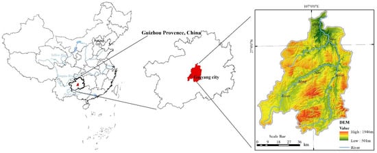
Figure 1. Location map of Qingshui River watershed with DEM.

3. Methodology

In the current study, ML algorithms comprising Back-Propagation Artificial Neural Networks (BP-ANN), Boosted Regression Trees (BRT), Random Forest (RF), and Support Vector Regression (SVR) were developed for evaluating soil erosion susceptibility based on field measurements and prior data of soil erosion empirical statistical models. The methodological flow chart of the study is as shown in Figure 2.

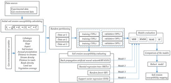
Figure 2. Methodological flow chart.

3.1. Data Collection

3.1.1. Experimental Data

In and around the Qingshui River watershed, there are 18 soil and water conservation experimental stations and 89 runoff plots (Figure 3). A total of 25 runoff plots, representing different slope gradients and planting configurations, were established to obtain experimental data in the Qingshui River watershed. The experimental data were collected from 2001 to 2011 across 18 hydrological stations in a karst region. Field plots were established across diverse topographic and management conditions, with slopes varying from 5° to over 45° and surface areas typically between 25 m² and 235 m². These plots represented distinct land use types: sloping cropland (maize, soybean, pepper), terraced land, and naturally vegetated land (1–95% cover); bare plots without conservation measures served as controls. Runoff and sediment were measured after each of the 10–25 rainfall-runoff events occurring per year, where events were separated by at least 6 h. Each station used self-recording rain gauges to log rainfall at 5-min intervals. The monitored parameters encompassed vegetation coverage (%), rainfall frequency, rainfall duration, cumulative rainfall time (min), total precipitation (mm), and rainfall intensity (mm/h), among others. Following each runoff event, measurements of runoff depth (mm) were taken in the diversion pool, while sediment concentration (kg·m⁻³) was quantified through laboratory analysis of samples collected from the collection pool.

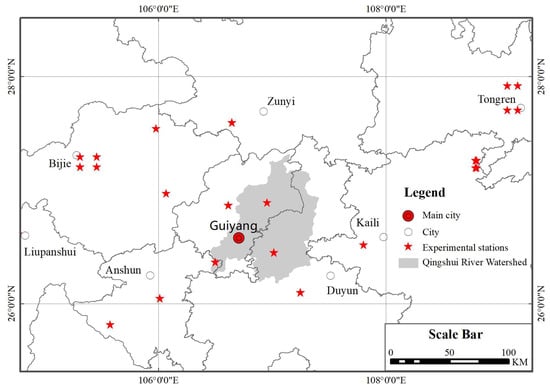
Figure 3. Soil and water conservation experimental stations.

The soil and water conservation monitoring infrastructure in the Qingshui River watershed also includes a sub-watershed control station, the Guiyang hydrological station and the Hefeng hydrological station, etc. Water level observations are made using a basic water gauge, a self-registering water level meter for flood level observations, and monitoring indicators that also include day-by-day runoff, sediment content, sediment production, and sediment production modulus for the sub-watershed. These experimental data provide reliable and consistent erosion measurements, which are a solid database for the soil erosion studies on the slope, sub-watershed, and regional scales. This experimental outcome also can be additionally employed to construct novel data-driven machine learning models for soil erosion susceptibility evaluation.

3.1.2. Geo-Environmental Factors

As mentioned above, owing to the complex nature of soil erosion mechanisms in karst ecological zones, the regional applicability of soil erosion susceptibility factors still needs to be studied in depth. The lithology, topography, soil condition, rainfall, hydrology, and human activities are all closely related to soil erosion.

(1)

Lithologic: The lithological setting serves as a primary factor shaping regional landforms, soils, and vegetation patterns. It significantly affects an area’s vulnerability to soil erosion, given that erosion mechanisms are strongly tied to the physicochemical characteristics of lithological materials exposed at the surface [38,39,40]. The lithological data used in this study were extracted from geological maps with a scale of 1:50,000. The identified lithologies consist of dolomite, dolomitic horizons, successions where dolomite alternates with clastic materials, lithologies outside the carbonate group, massive limestone, limestone containing thin interlayers, alternating strata of limestone and dolomite, limestone interbedded with clastic sediments, mixed carbonate–clastic rocks, and other carbonate–clastic interbedded units.

(2)

Topography: Topographic factors, particularly slope characteristics, exert a significant influence on the initiation and progression of soil erosion. Slope gradient is a key determinant in the formation of gullies, while slope aspect affects a range of environmental processes, including weathering intensity, soil moisture distribution, erosion rates, vegetation patterns, and overall geomorphological dynamics. The digital elevation model (DEM) applied in this research was constructed with a grid size of 30 m, and the dataset was sourced from the Geospatial Data Cloud platform (http://www.gscloud.cn/) (accessed on 1 November 2024). Using the DEM as a base dataset, key physiographic and geomorphological parameters—including elevation, slope, and aspect—were derived through spatial analysis in ArcGIS 10.8.

(3)

Soil texture: It is widely recognized that soil texture is an important control mechanism for runoff formation and infiltration, and therefore an important factor in the formation of depressions [41]. According to the soil census data for the study area, there are seven soil textures in the region, including silty clay loam, silt loam, loamy clay, rocks, and stony soil. The soil texture raster distribution map was generated by applying the data conversion tools within the ArcGIS software environment.

(4)

Water-related factors: Annual precipitation, proximity to stream channels, and stream density were incorporated into the analysis as representative hydrological factors to evaluate their impact on the initiation and subsequent development of soil erosion [42]. In this study, the stream network was delineated through hydrological analysis in ArcGIS using a 30 m resolution dataset. Based on this network, stream proximity and density layers were produced using the Euclidean Distance and Line Density tools available in ArcGIS 10.8.

(5)

Anthropogenic and Environmental Features:

(a)

Anthropogenic Factors: The anthropogenic activities significantly impact soil erosion initiation and development, for instance, roadways, where concentrated runoff often induces gully formation. During road construction, the natural drainage patterns are altered, and exposed soil becomes highly susceptible to erosion due to runoff accumulating on impermeable surfaces [2]. Therefore, A map depicting the distance from sites to nearby roads and road density were obtained with the ArcGIS10.8 distance function and Line density tools.

(b)

Hydrological and geomorphological processes are significantly influenced by land use, as these factors control the generation of surface runoff and the movement of sediments. The spatial pattern of land use in the study region was extracted from Landsat 7 ETM+ (30 m spatial resolution) satellite images through a supervised classification approach, and the interpretation was subsequently verified through field surveys. The land use was classified into nine primary categories: paddy field, arid land, garden area, forest, grassland, building land, bare ground, bare rock, and water. Environmental Factor: Vegetation Cover: Vegetation cover acts as an essential environmental factor controlling soil erosion, particularly in karst landscapes where vegetation stability directly affects slope erosion and sediment yield [43,44,45]. Vegetation coverage was calculated using the vegetation index NDVI, and the formula is as follows:

$$fv=(NDVI-NDV{I}_{\min })/(NDV{I}_{\max }-NDV{I}_{\min })$$

(1)

where fv indicates the proportion of vegetation cover, and NDVI stands for the normalized difference vegetation index, and $NDV{I}_{\min }$ and $NDV{I}_{\max }$ are the minimum and maximum value of the normalized vegetation index; the $NDV{I}_{\min }$ and $NDV{I}_{\max }$ cannot be taken directly from the maximum and minimum values counted from the NDVI grayscale maps, which should be determined considering the actual characteristics of the study area, image size, and image clarity in reference to relevant literature. In this paper, we take their empirical values of 0.1 and 0.85, respectively [46].

3.2. Soil Erosion Susceptibility Estimation Empirical Model

3.2.1. Conceptual Framework and Estimation of Soil Erosion Susceptibility Index

Applicability of the Modified Universal Soil Loss Model (RUSLE) in karst areas has been validated [47,48]. The soil erosion susceptibility in this study refers to the inherent spatial potential of an area to undergo soil loss under uniform external forcing, which depends mainly on relatively stable factors such as topography, soil, vegetation, and soil conservation measures. It should be distinguished from erosion risk, which represents the probability or likelihood of erosion occurrence under dynamic conditions, including rainfall intensity or land-use disturbance. Accordingly, the process of estimating the soil erosion susceptibility index (S_S) can be based on the empirical statistical model of RUSLE, considering the effects of rainfall, soil, topography, vegetation, and soil conservation management. To construct a dimensionless and comparable index for karst ecosystems, each factor is normalized and ranked, denoted as the ranked value of rainfall erosivity (Rᵣ), the ranked value of soil erodibility (Kᵣ), the ranked value of slope length and steepness (LSᵣ), the ranked value of vegetation cover (Cᵣ), and the ranked value of erosion mitigation practice intensity (Pᵣ). Each of these corresponds conceptually to the traditional RUSLE parameters (R, K, LS, C, and P), but the subscript “ᵣ” denotes their normalized, ranked form under karst conditions. The multiplicative integration of these dimensionless indices follows the empirical form proposed by Zhou et al. [49] and conceptually extended in Zhang et al. [32] and Mo et al. [50]. The soil erosion susceptibility index (S_S) is calculated using the following formula:

$$S_s=\sqrt[5]{R_r\ast K_r\ast L{S}_r\ast C_r\ast P_r}$$

(2)

This composite index provides a quantitative estimate of soil vulnerability to erosion, facilitating a systematic assessment of spatial variability in erosion risk across the target area.

3.2.2. Impact Factors

(1)

Rainfall erosivity factor (R): The rainfall erosivity factor represents the potential of precipitation, either over a specific time period or from a single storm event, to cause soil erosion. Using the experimental rainfall data collected at 5 min intervals, the peak 30 min rainfall rates (mm/h) and the corresponding rainfall erosivity (R, MJ·mm/(ha·h)) were calculated using the following equation [45,51]:

$$R=E{I}_{30}$$

(3)

$$E=\sum _{r=1}^n(e_r\cdot p_r)$$

(4)

$$e_r=0.29\left[1-0.72\mathit{exp}(-0.082i_r)\right]$$

(5)

In this study, $I_{30}$ represents the highest 30 min rainfall intensity (mm/h) and corresponds to the total kinetic energy of the storm MJ/(ha·mm). Each rainfall event is subdivided into n intervals based on variations in rainfall intensity. Within the r-th interval, $P_r$ corresponds to the precipitation amount (mm), $e_r$ indicates rainfall kinetic energy normalized by unit rainfall depth (MJ/ha.mm), and $i_r$ represents the rainfall intensity (mm/h) during that interval.

(2)

Soil erodibility factor (K): Soil erodibility (K) is the property of a soil that makes it susceptible to damage by erosion. The K factor characterizes the influence of soil properties on erosion processes. The larger the K, the less vulnerable it becomes to soil erosion, and the smaller the K, the more susceptible the soil is. The K value is related to the type of soil, the texture of the soil, and the content of soil organic matter. The K value can be estimated based on organic carbon content and particle size distribution data derived from the results of soil survey [52], and the K value distribution map can be obtained by spatial interpolation.

$$K=\left\{0.2+0.3{\mathit{exp}}^{\left[-0.0256S_a\left(1-{\displaystyle \frac{S_i}{100}}\right)\right]}\right\}\times ({\displaystyle \frac{S_i}{C_l+S_i}}{)}^{0.3}\left[1-{\displaystyle \frac{0.25C}{C+\mathit{exp}\left(3.72-2.95C\right)}}\right]\times \left[1-{\displaystyle \frac{0.7S_n}{S_n+\mathit{exp}\left(-5.51+22.9S_n\right)}}\right]$$

(6)

where K—soil erodibility factor; S_a—percentage of sand particles (0.05–2.0 mm); Sᵢ—percentage of silt particles (0.002–0.05 mm); Cₗ—percentage of clay particles (<0.002 mm); C—organic carbon content (%); S_n—a normalized sand fraction defined as S_a/100; and exp—exponential function.

(3)

Slope length–steepness factor (LS). The LS factor incorporates the impacts exerted by both slope length (L) and slope gradient (S). ArcGIS10.8 spatial analyst function was taken into consideration to estimate the LS factor. Considering the equation of Moore and Burch [53], the L factor was estimated:

$$L=(Flow Accumulation\times Cell Size/22.13{)}^M$$

(7)

where L denotes the slope length factor and M represents the slope length index, and an $M$ value of 0.5 was adopted in the text, as it is suitable for estimating slope length under steeper terrain conditions.

The following equations were used to calculate the slope steepness factor (S) [54]:

$$s=\left\{\begin{array}{c}10.8sin\alpha +0.03 \alpha <5°\\ 16.8sin\alpha -0.5 5°\le \alpha <10°\\ 21.9sin\alpha -0.96 \alpha \ge 10°\end{array}\right.$$

(8)

where S is the slope steepness factor and $\alpha$ is the slope degree value.

(4)

Vegetation management factor (C). The C factor refers to the ratio of soil loss from cultivated land under specific farming practices to that from bare soil under continuous fallow conditions [7]. In soil research, the C factor not only mitigates soil erosion but also contributes to soil and water conservation, and its values generally range between 0 and 1. The larger the value of C, the greater the amount of soil erosion. For the assessment of vegetation coverage (fv), this study employed China’s 30 m resolution annual maximum NDVI dataset (1986–2024), which is based on U.S. Landsat remote sensing imagery. The NDVI data for 2023 were used in this study. The method described by Karydas et al. and Tian et al. was then employed to determine the C value [55,56], which was obtained by calculating the vegetation coverage (fv) to establish a linear regression equation [57].

$$\left\{\begin{array}{c}C=1\hspace{0.33em}\hspace{0.33em}\hspace{0.33em}\hspace{0.33em}\hspace{0.33em}\hspace{0.33em}\hspace{0.33em}\hspace{0.33em}\hspace{0.33em}\hspace{0.33em}\hspace{0.33em}\hspace{0.33em}\hspace{0.33em}\hspace{0.33em}\hspace{0.33em}\hspace{1em}fv=0\hfill \\ C=0.6508-0.3436\mathit{lg}fv\hspace{0.33em}\hspace{0.33em}\hspace{0.33em}\hspace{0.33em}\hspace{0.33em}0<fv<78.3\%\hfill \\ C=0\hspace{0.33em}\hspace{0.33em}\hspace{0.33em}\hspace{0.33em}\hspace{0.33em}\hspace{0.33em}\hspace{0.33em}\hspace{0.33em}\hspace{0.33em}\hspace{0.33em}\hspace{0.33em}\hspace{0.33em}\hspace{0.33em}\hspace{0.33em}\hspace{0.33em}\hspace{1em}fv>78.3\%\hfill \end{array}\right.$$

(9)

where C denotes the cover management factor, whereas fv is the fractional vegetation coverage ratio. When the vegetation coverage is over 78.3%, the amount of surface erosion is extremely weak, and the value of C is recorded as 0. When the vegetation coverage equals to 0, the value of C is 1.

The threshold value of 78.3% was adopted following the empirical results of Schönbrodt et al. [58], who reported that in a mountainous watershed in Central China, the regression between the C-factor and vegetation cover reached a minimum near zero when the fractional vegetation cover (FVC) ≈ 78.3%. This relationship has also been validated in karst regions, where vegetation coverage effectively limits soil detachment despite the influence of lithological and hydrological heterogeneity [59,60]. Therefore, the adoption of the 78.3% threshold in this study is reasonable and applicable to karst terrain conditions.

(5)

The conservation practice factor (P). The P factor quantifies the impact of soil and water conservation measures. These interventions are designed to lower runoff quantity and flow rate, which consequently diminishes the potential for soil erosion [55,61]. The P factor generally varies between 0 and 1. A p value of 0 signifies complete prevention of soil erosion in the area, while a value of 1 indicates the absence of any erosion control measures. In this study, P-factor values were determined according to land use types extracted from 2020 Landsat 8 OLI images (30 m resolution). The images were atmospherically corrected and verified using field observations. Based on visual interpretation, the study area was classified into sloping cropland, terraced fields, and naturally vegetated land. Sloping cropland was further divided into plots with or without soil conservation measures, such as contour tillage and grass strips. Accordingly, a p value of 1.0 was assigned to sloping cropland lacking conservation measures and to naturally vegetated areas, 0.01 to terraced land, and 0.2–0.7 to sloping cropland adopting contour farming or other mechanical or vegetative practices [62,63]. The P-factor map was produced by reclassifying the land-use raster based on these criteria to maintain consistency with the RUSLE computation grid.

3.3. Machine Learning Algorithms

The present study employed four prominent and potentially applicable machine learning techniques, namely a back-propagation artificial neural network (BPANN), two tree-based ensemble methods—boosted regression trees (BRT) and random forest (RF)—and support vector regression (SVR), to quantitatively evaluate soil erosion susceptibility.

(1)

Back-propagation artificial neural network (BPANN): BPANN is a multilayer feedforward network trained using the error back-propagation algorithm, and it remains one of the most widely adopted learning methods for multilayer ANN architectures [64]. Through modifications to the learning rate and the quantity of hidden nodes, the BP algorithm calculates the connection weights from the input layer, through the hidden layer, and finally to the output layer. The training of the neural network is conducted by iteratively updating these weights so as to reduce the error between the model’s predicted values and the actual outputs [65,66].

(2)

Boosted regression trees (BRTs): BRTs are fitted statistical models that combine the two methods of regression trees and boosting [67]. Boosting is a powerful ensemble method that improves predictive performance through an iterative process of training new trees to correct errors made by prior models. It can be regarded as an additive regression approach, where each simple tree is incorporated step by step in a forward manner [68]. The BRT model constructs an ensemble of multiple trees, which not only overcomes the inherent shortcomings of single-tree methods but also integrates their strengths to achieve reduced model variance and enhanced predictive performance [69].

(3)

Random forest (RF): The RF is a nonparametric multivariate approach that can be employed for performing regression as well as classification, interaction detection, clustering, and variable selection [70,71]. This algorithm generates thousands of trees so as to develop a ‘forest’. The growth of each tree is achieved through the regression tree method, based on bootstrap samples of the data. Additionally, at each node position, a random subset of variables is selected. Based on the majority vote among all decision trees, the final model is constructed [72]. The model offers several advantages, including independence from data distributional assumptions, low computational demands, reduced risk of overfitting, suitability for high-dimensional datasets, and superior predictive accuracy [73].

(4)

Support Vector Regression (SVR): SVR is a regression technique developed within the framework of Support Vector Machines (SVM). SVM is an important machine learning model, with the advantages of self-learning ability, global minimum, insensitivity to changes in input data, nonlinear mapping, etc., and it also has stronger advantages in establishing the correlation prediction model than the traditional prediction model [74]. There are two core classifications of Support Vector Machine (SVM): one is Support Vector Classification (SVC) for classification tasks, and the other is Support Vector Regression (SVR) for regression tasks. SVR has a distinct characteristic: rather than minimizing the training error of observed values, it attempts to reduce the generalized error bound to the lowest possible level, thereby achieving generalized performance [75]. Studies on SVR indicate that this method serves as an effective alternative for approximating intricate engineering computations, delivering superior accuracy and enhanced robustness in function fitting [76].

3.4. Evaluation Criteria of Model Performance

Model evaluation is an integral and important part of developing effective models, which helps to identify and select good models so as to enhance prediction accuracy. Here, A suite of performance metrics—namely, root mean square error (RMSE), mean absolute error (MAE), and R-squared (R²)—was employed to evaluate the validity and efficacy of the developed models. Of the three parameters, RMSE and MAE are widely adopted as dimensional statistical measures, primarily used to assess the performance of models producing continuous output values. Both RMSE and MAE quantify the average discrepancies between model outputs and actual measurements in the same units as the model outputs. In contrast, the coefficient of determination (R²) evaluates the goodness-of-fit of the regression line, with higher R² values indicative of a stronger correspondence between the model predictions and observed data.

RMSE is the square root of the expected value of the average squared difference between the predicted and the observed values. Lower values of this metric correspond to higher model accuracy. RMSE can be written as follows:

$$RMSE=\sqrt{{\displaystyle \frac{1}{m}}{\sum }_{i=1}^m(y_i-{\widehat{y}}_i{)}^2}$$

(10)

MAE is calculated by averaging the absolute differences between predicted and observed values. It provides a more direct reflection of prediction errors, with smaller values indicating higher model accuracy.

$$MAE={\displaystyle \frac{1}{m}}{\sum }_{i=1}^m\left|y_i-{\widehat{y}}_i\right|$$

(11)

The R² value indicates the agreement between predicted and measured values on the regression line. R² ranges from 0 to 1. The higher the R², the better the models simulate the results, and the predictive model is considered “perfect” if the value is equal to 1. R² is defined as follows:

$$R^2=1-{\displaystyle \frac{{\sum }_{i=1}^m(y_i-{\widehat{y}}_i{)}^2}{{\sum }_{i=1}^m(y_i-{\stackrel{-}{y}}_i{)}^2}}$$

(12)

where $y_i$ is the recorded soil erosion susceptibility index, ${\widehat{y}}_i$ represents the output value from the model, ${\stackrel{-}{y}}_i$ is the mean of the recorded erosion susceptibility, and $m$ is the number of sampling points.

4. Results

4.1. Soil Erosion Susceptibility Assessment Based on RUSLE Model

Following the RUSLE framework, the erosion-related factors were quantified and spatially represented using GIS analysis. The geographical variation of each factor considered in the erosion model is illustrated in Figure 4, as follows: panel (a) shows factor R (rainfall erosivity), (b) displays the LS factor, (c) corresponds to factor K (soil erodibility), (d) presents factor C (cover management), and (e) illustrates factor P (conservation practices). Each factor was reclassified into five susceptibility levels (very low, low, moderate, high, and very high) based on the criteria established in Table 1.

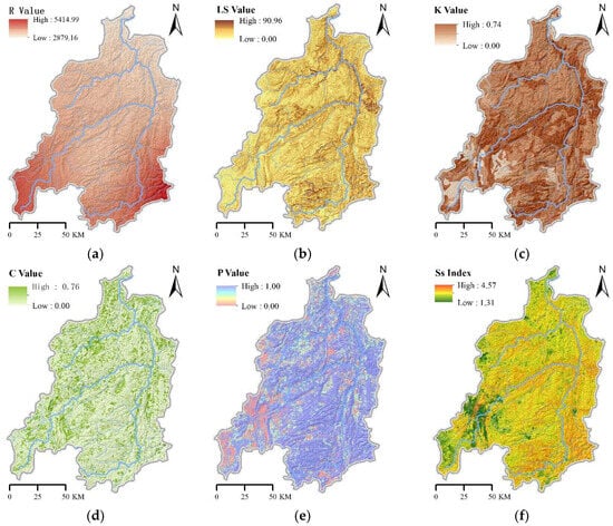
Figure 4. Distribution maps of RUSLE-related factors and the soil erosion susceptibility index. Following the RUSLE framework, erosion-related factors were quantified and spatially represented using GIS analysis. The geographical variation of each factor is illustrated as follows: (a) R factor (rainfall erosivity); (b) LS factor; (c) K factor (soil erodibility); (d) C factor (cover management); (e) P factor (conservation practices); (f) S_S factor.

Table 1. Classification standard of soil erosion susceptibility.

Factors	Very Low	Low	Moderate	High	Very High
Rank Value	1	2	3	4	5
R	≤2000	2000–3000	3000–4000	4000–5000	>5000
K	0	0–0.20	0.20–0.40	0.40–0.60	>0.60
LS	≤10	10–20	20–30	20–30	>30
C	0	0–0.15	0.15–0.30	0.30–0.60	>0.60
P	0	0–0.35	0.35–0.60	0.60–0.80	>0.80

Based on the empirical statistical model of RUSLE, the soil erosion susceptibility index (S_S) was calculated, with values ranging from 1.31 to 4.57 (Figure 4f). High susceptibility is mainly concentrated in the southern watershed and steep-slope areas, whereas the lowest values occur in the southwest. This contrast underscores the significant spatial variability of erosion risk within the study area.

4.2. Spatial Mapping of Predictive Factors and Machine Learning Sample Datasets

To better capture the multifaceted drivers of soil erosion in karst ecological zones, twelve explanatory variables were incorporated into the machine learning analysis, representing lithology, terrain, soil properties, rainfall, hydrological conditions, and human activities. The spatial distribution of these factors—lithology, elevation, slope, aspect, soil texture, annual rainfall, distance to rivers, river density, distance to roads, road density, land use type, and vegetation coverage—is presented in Figure 5, offering a comprehensive representation of environmental variability within the study region.

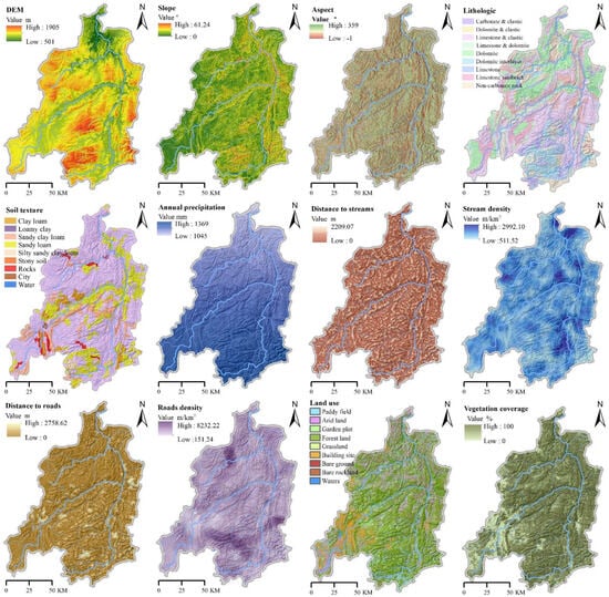
Figure 5. Distribution maps of geo-environmental factors.

To develop the machine learning models, three independent datasets (DS1, DS2, and DS3) were generated through iterative spatial random sampling. A total of 1160 documented soil erosion cases were compiled, and each dataset was divided into training and validation subsets at an approximate ratio of 70:30. This process resulted in 812 samples (70%) for training and 348 samples (30%) for validation within each dataset. The spatial distribution of the sampled points is illustrated in Figure 6, with training and validation points displayed. The sampling approach effectively captured the environmental heterogeneity of the study region, with sample sites broadly distributed across different lithological units, topographic gradients, and land-cover categories. This representative coverage guarantees that the machine learning models are trained and validated on a balanced subset of the landscape, thereby enhancing the credibility of the susceptibility assessment.

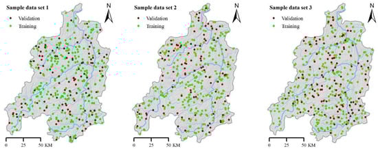
Figure 6. Distribution maps of three sample data sets.

4.3. Soil Erosion Susceptibility Machine Learning Models and Validation

The BPANN, BRTs, RF and SVR soil erosion susceptibility models were constructed utilizing the three training subsets of the sample DS1, DS2, and DS3 in the training steps, respectively. A network with one hidden layer containing 12 nodes was selected, using the ReLU activation function and the Adam optimizer with a learning rate of 0.001. For BRT, we used 150 trees, a learning rate (shrinkage) of 0.01, and an interaction depth of 3. For RF, the model comprised 150 trees, with the number of features considered at each split set to the square root of the total features. The radial basis function (RBF) kernel was selected. The optimal regularization parameter (C) was 10, and the kernel coefficient (gamma) was 0.1. Model performance was assessed on the corresponding validation subsets by comparing predicted and observed values. Table 2 summarizes the performance metrics (RMSE, MAE, and R²) for all models across the three datasets.

Table 2. Performance metrics of the models.

Data Set	Index	BPANN		BRTs		RF		SVR
		Train	Test	Train	Test	Train	Test	Train	Test
DS2	RMSE	0.680	1.230	0.081	0.119	0.187	0.234	0.790	0.871
	MAE	0.170	0.263	0.036	0.085	0.101	0.186	0.114	0.206
	R2	0.515	0.463	0.996	0.816	0.843	0.673	0.445	0.464
DS2	RMSE	0.493	0.867	0.368	0.733	0.374	0.816	0.798	1.062
	MAE	0.076	0.115	0.032	0.107	0.035	0.163	0.263	0.669
	R2	0.545	0.422	0.858	0.616	0.815	0.642	0.431	0.417
DS3	RMSE	0.574	0.816	0.033	0.065	0.374	0.463	0.433	0.865
	MAE	0.236	0.307	0.101	0.107	0.132	0.194	0.201	0.494
	R2	0.654	0.543	0.929	0.736	0.854	0.603	0.499	0.416
Average	RMSE	0.582	0.971	0.161	0.306	0.312	0.504	0.674	0.933
	MAE	0.161	0.228	0.056	0.100	0.090	0.181	0.193	0.456
	R2	0.571	0.476	0.928	0.723	0.837	0.639	0.458	0.432

The results calculated by three varied stratified random sampling methodologies show clear differences among the four algorithms. The average RMSE of the training data for the BPANN, BRTs, RF, and SVR models is 0.582, 0.161, 0.312, and 0.674, respectively, with BRT and RF achieving substantially lower errors than BPANN and SVR. Nevertheless, when applied to the test dataset, the mean RMSE values for the BPANN, BRTs, RF, and SVR models on the test data increased to 0.971, 0.306, 0.504, and 0.933, respectively. suggesting possible overfitting in some models, particularly for BPANN and SVR. By contrast, the BRT and RF algorithms showed limited signs of overfitting and consistently outperformed the BPANN and SVR models in terms of predictive capability.

The MAE results of the four models generally corroborated the previous observations. For the training dataset, the average MAE values for BPANN, BRT, RF, and SVR were 0.161, 0.056, 0.090, and 0.193, respectively, indicating that BRT and RF outperformed BPANN and SVR. For the test dataset, the corresponding average MAE values increased to 0.228, 0.100, 0.181, and 0.456, respectively, reflecting larger prediction errors compared with the training data. The R² value also indicated that BRT was the top-performing model, followed by RF, BPANN, and SVR. The average R² of the learning data for the BPANN, BRTs, RF, and SVR models were 0.571, 0.928, 0.837, and 0.458, respectively. The average R² of the test data for the BPANN, BRTs, RF and SVR models fell to 0.476, 0.723, 0.639, and 0.432, respectively. Overall, BRT consistently delivered the highest predictive accuracy, with RF as the second-best performer. These two algorithms should be given priority for subsequent spatial mapping of soil erosion susceptibility.

4.4. Geo-Environmental Variables Importance Analysis

The relative influence of geospatial environmental variables contributing to soil erosion was quantitatively evaluated through the application of model-specific variable importance metrics. For the Random Forest (RF) model, variable importance was calculated based on the mean decrease in Gini impurity. For the Boosted Regression Trees (BRTs), importance was derived from the relative influence metric, which sums the number of times a variable is used for splitting, weighted by the squared improvement. Since Support Vector Regression (SVR) lacks a native importance function, we employed a permutation importance technique, where the increase in root means square error (RMSE) after randomly permuting each predictor was used as the importance measure. For the Back-Propagation Artificial Neural Network (BPANN), permutation importance was also applied to ensure comparability across models. The average relative importance of the soil erosion geo-environmental variables was obtained based on the three training datasets running result (Figure 7).

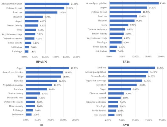
Figure 7. Geo-environmental variables relative importance statistical chart.

In the BPANN model, the most influential factors contributing to soil erosion susceptibility are annual precipitation (21.40%), distance to roads (19.00%), land use (15.70%), and elevation (8.70%). The BRTs model also identified annual precipitation (19.10%) as the most critical factor, with aspect (14.60%), distance to roads (12.20%), and land use type (10.60%) being secondary. In contrast, the RF model prioritized aspect (17.30%) above annual precipitation (14.80%), slope (14.00%), and stream density (12.50%). For the Support Vector Regression (SVR) model, land use ranks highest in importance (15.00%), followed by annual precipitation (13.20%), stream density (10.90%), and vegetation coverage (10.70%).

Although the ranking of variable importance varies among models, several key environmental factors—such as annual precipitation, land use, aspect, slope, and stream density—were consistently identified as highly influential across all four algorithms. This indicates that while each model emphasizes different dominant drivers due to their underlying learning mechanisms, they collectively highlight a common set of hydrological, topographic, and anthropogenic variables as the primary controls on soil erosion susceptibility in the study area.

4.5. Soil Erosion Susceptibility Mapping

Following the successful validation of the four machine learning models—BPANN, BRT, RF, and SVR—a soil erosion susceptibility map (SESM) was generated by leveraging pixel-level predictions across the entire study area. The resulting map was subsequently classified into five distinct susceptibility categories (very low, low, moderate, high, and very high) employing the Natural Breaks algorithm in ArcGIS 10.8. Figure 8 visually summarizes the spatial distribution of the classified susceptibility levels.

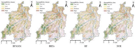
Figure 8. Soil erosion susceptibility maps based on ML models.

Table 3 presents the statistical features of the predicted probabilities for the spatial extent of soil erosion susceptibility, classified into progressively increasing risk levels: very low, low, moderate, high, and very high, as derived from the attributes of the susceptibility maps. The predicted susceptibility values from each model were grouped into five categories using the Jenks natural breaks approach, which determines natural groupings within the data to minimize intra-class variance and maximize inter-class differences. Such a classification better represents the spatial variation in erosion susceptibility and aligns with methods applied in other karst area studies [76]. The BPANN model estimates the area coverage corresponding to very low to very high soil erosion susceptibility classes as follows: 544.08 km² (8.22%), 835.32 km² (12.62%), 1749.40 km² (26.43%), 2302.75 km² (34.79%), and 1187.45 km² (17.94%), respectively. The BRT model results show a greater concentration in high-value zones, with high and extremely high-susceptibility zones collectively comprising 64.2%, whilst extremely low and low susceptibility levels are confined to limited areas in the southwest. Similarly, the RF model indicates that a substantial portion of the area is classified as highly susceptible to soil erosion. The areal extents for minimal, slight, moderate, considerable, and extreme susceptibility zones are 347.50 km² (5.25%), 743.31 km² (11.23%), 1531.64 km² (23.14%), 2662.16 km² (40.22%), and 1334.39 km² (20.16%), respectively. In contrast, the SVR model’s predictions were somewhat more moderate, with medium and high susceptibility levels comprising about 61%, though the proportion of extremely high-susceptibility areas (16.1%) was lower than that predicted by BRT and RF.

Table 3. Soil erosion susceptibility statistical characteristics of the classes’ area.

Susceptibility Class	BPANN		BRTs		RF		SVR
	Km2	%	Km2	%	Km2	%	Km2	%
Very low	544.08	8.22	300.50	4.54	347.50	5.25	499.07	7.54
Low	835.32	12.62	662.56	10.01	743.31	11.23	993.51	15.01
Moderate	1749.40	26.43	1406.54	21.25	1531.64	23.14	1867.88	28.22
High	2302.75	34.79	2853.45	43.11	2662.16	40.22	2193.54	33.14
Very high	1187.45	17.94	1395.95	21.09	1334.39	20.16	1065.00	16.09
Total	6619.00	100.00	6619.00	100.00	6619.00	100.00	6619.00	100.00

Overall, all four models consistently indicate that a significant portion of the study area falls within the moderate to high soil erosion susceptibility categories, while only the southwestern region and certain areas with gentle slopes exhibit very low or low sensitivity. The primary variation among the models pertains to the spatial extent and proportion of high-sensitivity zones, with the BRT and RF models identifying the most extensive high-susceptibility regions.

5. Discussion

5.1. Soil Erosion Susceptibility Estimation Models

Currently, there is no universally accepted model for predicting regional soil erosion susceptibility. Most assessments rely on empirical equations, selecting sensitivity indicators and integrating them through weighted or unweighted overlay methods to map spatial susceptibility patterns [77]. However, these traditional approaches can only handle limited variables, and multicollinearity among factors often reduces accuracy [39]. In contrast, machine learning (ML) methods provide greater flexibility by accommodating multiple explanatory variables, integrating multi-scale data, and effectively modeling complex nonlinear relationships.

Among the four machine learning models applied in this study, the Boosted Regression Tree (BRT) demonstrated the highest predictive performance (R² = 0.928, RMSE = 0.306, MAE = 0.261). Its superiority can be attributed to three key algorithmic features. First, BRT combines regression trees with boosting techniques, enabling it to effectively capture the complex nonlinear interactions among hydrological, lithological, and anthropogenic factors in karst landscapes. Second, its adaptive boosting process iteratively minimizes residual errors, thereby improving the model’s robustness and generalization ability. Finally, the built-in regularization helps prevent overfitting caused by multicollinearity among variables. These advantages explain why the BRT model outperformed the Random Forest, Backpropagation Neural Network, and Support Vector Regression models in this research.

The present findings are consistent with previous research applying ML models for erosion or landslide susceptibility mapping in karst or mountainous regions. For instance, Nguyen et al. [35] found that BRTs outperformed RF and ANN models due to their superior handling of nonlinear dependencies. Similarly, Conforti et al. [39] emphasized that ensemble tree-based models are particularly effective in capturing the combined influence of hydrological and geomorphological factors. Compared with these studies, our work further demonstrates the robustness of BRTs under the highly variable environmental conditions of Southwest China’s karst area, highlighting the algorithm’s strong adaptability to fractured terrain and heterogeneous soil–rock structures.

This study has certain limitations. First, due to data availability constraints, essential soil physicochemical properties such as organic matter content and infiltration capacity were not incorporated, which may have affected the precision of the erosion susceptibility assessment. Second, although the machine learning models achieved high predictive accuracy, their limited capacity to represent physical processes restricts deeper insights into the underlying mechanisms driving soil erosion. Future studies should aim to address these limitations by integrating time-series data (e.g., rainfall erosivity, vegetation phenology) and hydro-geomorphological process models with ML algorithms to improve both accuracy and interpretability. Incorporating field-based soil erosion measurements and remote-sensing time series would also strengthen model calibration and validation.

5.2. Variable Importance in the Susceptibility Models

In the modeling process of this study, different models exhibited both consistency and variability in identifying the key geo-environmental factors influencing soil erosion susceptibility. Based on the results from the BPANN, BRTs, RF, and SVR models, hydrological factors (e.g., annual precipitation), topographic factors (e.g., slope, aspect, elevation, stream density), and anthropogenic factors (e.g., land use, distance to roads) generally showed high importance. The outcome corroborates the conclusions drawn in Zhang Enwei et al. [33], highlighting that the identification of critical geo-environmental variables plays a decisive role in improving model performance.

The strong influence of precipitation is particularly evident in the karst mountain setting of the study area. In karst terrains, the combination of steep slopes, thin soils, and highly fractured carbonate rocks enhances surface runoff and limits water retention, making rainfall the principal trigger for soil detachment and sediment transport. Rapid infiltration through fissures and sinkholes further intensifies hydrological variability, creating alternating zones of concentrated overland flow and subsurface drainage. These hydrological characteristics amplify the erosive impact of precipitation events and explain why rainfall-related factors dominate the susceptibility models.

Topography exerts an equally important but more localized control on erosion potential. The steep gradient of the Qingshui watershed increases runoff velocity and shear stress, promoting the formation of rills and gullies on exposed slopes. Slope and aspect influence how rainfall energy is distributed, while elevation modulates both precipitation intensity and vegetation cover. In this context, the interplay between precipitation and terrain governs the spatial variability of soil erosion, rather than either factor acting independently.

The type of land utilization and surface coverage plays an essential role in maintaining slope geomorphic stability. Regions with sparse vegetation or extensive road networks offer minimal resistance to raindrop impact and runoff, rendering them highly susceptible to erosion. Roads, in particular, modify natural drainage pathways and accelerate sediment movement along cut slopes and embankments. These anthropogenic influences highlight the importance of land management in maintaining slope stability within the karst environment.

Building on this approach, the results collectively indicate that soil erosion in this karst basin is not governed by a singular factor but through the interaction of terrain conditions, hydrological processes, and human activities. The findings demonstrate that precipitation–topography coupling is the dominant mechanism controlling erosion intensity and spatial heterogeneity in karst landscapes. This study provides new empirical evidence supporting the use of machine learning models to disentangle the relative importance of complex environmental drivers. Such complexity emphasizes the importance of integrated management strategies that target slope stabilization, sustainable land use planning, and the careful control of infrastructure development to reduce erosion risks in this ecologically fragile landscape.

5.3. Soil Erosion Susceptibility Characteristics and Spatial Differentiation

Previous studies have shown that most areas in Guizhou Province exhibit high soil erosion susceptibility, particularly in the central karst hill region, where geomorphological, climatic, and anthropogenic factors jointly contribute to severe erosion risk [78]. In this context, the estimated results of soil erosion susceptibility derived from the four ML models—BPANN, BRTs, RF, and SVR—demonstrate both consistent trends and noticeable variations in spatial patterns and severity levels across the Qingshui River watershed. Overall, all models indicate that a significant portion of the study area falls within the moderate to high susceptibility classes. Specifically, the BPANN model identifies 61.22% of the watershed as being within the elevated to severe risk categories, while BRTs and RF estimate these two categories to cover 64.20% and 60.38% of the area, respectively. The SVR model shows a slightly more balanced distribution, with high and very high zones accounting for 49.23% of the total area. This consistent emphasis on moderate to very high classes suggests that the Qingshui River watershed is generally at considerable risk of soil erosion, especially under intense rainfall and slope conditions.

As illustrated in the soil erosion susceptibility maps (Figure 8), soil erosion susceptibility in the Qingshui River watershed exhibits clear spatial heterogeneity. Overall, high-susceptibility areas are mainly concentrated along the central river corridors, the flanks of major tributaries, and the northern hilly regions, along with certain southern sections of the basin. These regions are characterized by steep slopes, extensive karst exposures, sparse vegetation cover, and rapid surface runoff—conditions that significantly favor gully formation and surface erosion. The karst landscape, with its underground drainage networks and sinkholes, further intensifies water concentration and accelerates soil detachment. Although all models reveal similar overall spatial patterns, the extent and connectivity of the susceptibility zones differ noticeably among them. The BPANN-derived map depicts relatively extensive and continuous high-susceptibility belts distributed across hilly and sub-basin regions. In contrast, the BRT model concentrates high-risk areas mainly along steep slopes, emphasizing its strong sensitivity to terrain gradients. The RF prediction exhibits smoother spatial transitions between susceptibility levels and provides a clearer distinction of moderate-risk areas, while the SVR result shows more scattered and discontinuous high-susceptibility patches. These variations demonstrate the divergent spatial responses of the models to nonlinear processes and interactions among environmental variables, despite their consistent overall susceptibility trends.

Alternatively, areas with “very low” and “low” susceptibility are primarily located in the southwestern and some south parts of the basin, as well as in flatter river valley zones. These areas are generally dominated by forested land use, with gentle slopes and better soil stability, making them less prone to erosion. This spatial distribution is closely associated with land use configuration, slope patterns, and drainage density, highlighting the compound effects of natural terrain and human influence on erosion risk.

These results indicate that soil erosion in the Qingshui River karst watershed arises from the interplay of precipitation, topography, land use, and subsurface karst structures, rather than a single controlling factor. The models quantify how these elements interact to produce spatially heterogeneous erosion patterns, confirming the roles of slope and vegetation while revealing how karst-specific features intensify erosion. This understanding offers practical guidance for targeted soil and water conservation in sensitive karst environments.

6. Conclusions and Perspectives

This study systematically compared the performance of four commonly used machine learning models—Random Forest (RF), Boosted Regression Trees (BRTs), Back-Propagation Artificial Neural Network (BP-ANN), and Support Vector Machine (SVM)—for assessing soil erosion susceptibility in the Qingshui River Basin, Guizhou Province, and quantitatively assessed the relative importance of geo-environmental variables affecting erosion susceptibility. The results demonstrate that (1) the Boosted Regression Trees (BRT) model consistently outperformed their counterparts in terms of predictive accuracy and stability, followed by the Random Forest (RF) model, whereas BPANN and SVR performed relatively weaker; (2) annual precipitation, land use, distance to roads, slope, aspect, elevation, and drainage density were the most influential factors and were identified as the dominant factors controlling the spatial distribution of erosion susceptibility. Hydrological and topographic variables jointly determine potential erosion intensity, while human activities such as road construction and land-use change intensify local erosion risks; (3) the susceptibility maps produced successfully pinpoint areas at high risk of topsoil loss, providing a valuable resource for environmental management, land use planning, and infrastructure development. Overall, this research clarifies the spatial heterogeneity and controlling mechanisms of soil erosion in karst hilly landscapes; the proposed modeling framework exhibits strong transferability and applicability, offering a useful tool for erosion risk identification and sustainable watershed management in other karst environments.

To advance the predictive capability of erosion susceptibility models, future research should focus on integrating multi-temporal remote sensing data, rainfall erosivity dynamics, and land use change trajectories to capture temporal dynamics. Coupling these enhanced data streams with process-based erosion models through machine learning techniques could enhance process understanding and prediction reliability. Finally, incorporating uncertainty analysis and spatial validation using field-based observations would further strengthen model generalization. Such measures will help to gain a more comprehensive understanding of soil erosion dynamics and provide support for sustainable basin management in fragile karst landform areas.

References

- Koch, A.; McBratney, A.; Adams, M.; Field, D.; Hill, R.; Crawford, J.; Minasny, B.; Lal, R.; Abbott, L.; O’Donnell, A.; et al. Soil Security: Solving the Global Soil Crisis. Glob. Policy 2013, 4, 434–441. [Google Scholar] [CrossRef]
- Zhan, C.S.; Jiang, S.S.; Sun, F.B.; Jia, Y.W.; Yue, W.F.; Niu, C.W. Quantitative contribution of climate change and human activities to runoff changes in the Wei river basin, China. Hydrol. Earth Syst. Sci. 2014, 11, 2149–2175. [Google Scholar]
- Amundson, R.; Berhe, A.A.; Hopmans, J.W.; Olson, C.; Sztein, A.E.; Sparks, D.L. Soil and human security in the 21st century. Science 2015, 348, 1261071. [Google Scholar] [CrossRef]
- Lal, R.; Pimentel, D. Soil erosion: A carbon sink or source? Science 2008, 319, 1040–1042. [Google Scholar] [CrossRef]
- Park, S.; Oh, C.; Jeon, S.; Jung, H.; Choi, C. Soil erosion risk in Korean watersheds, assessed using the revised universal soil loss equation. J. Hydrol. 2011, 399, 263–273. [Google Scholar] [CrossRef]
- Xu, H.; Zhu, X.; Borrelli, P.; Cao, L.; Shao, M. Current status and medium- and long-term variation of soil erosion by water in China. Geosustainability 2025, 6, 100372. [Google Scholar]
- Wischmeier, W.H.; Smith, D.D. Predicting Rainfall Erosion Losses; USDA: Washington, DC, USA, 1978; Agricultural Handbook No. 537.
- Liu, B.Y.; Xie, Y.; Zhang, K.L. Soil Erosion Prediction Model; China Science and Technology Press: Beijing, China, 2001. [Google Scholar]
- Yan, J.; Wang, S.; Feng, J.; He, H.; Wang, L.; Sun, Z.; Zheng, C. New 30-m resolution dataset reveals declining soil erosion with regional increases across Chinese mainland (1990–2022). Remote Sens. Environ. 2025, 323, 114681. [Google Scholar]
- Yin, C.; Bai, C.; Zhu, Y.; Shao, M.; Han, X.; Qiao, J. Future soil erosion risk in China: Differences in erosion driven by general and extreme precipitation under climate change. Earth Future 2025, 13, e2024EF005390. [Google Scholar] [CrossRef]
- Zheng, M.; Cai, Q.; Cheng, Q. Modelling the runoff-sediment yield relationship using a proportional function in hilly areas of the Loess Plateau, North China. Geomorphology 2008, 93, 288–301. [Google Scholar] [CrossRef]
- Beasley, D.B.; Huggins, L.F.; Monke, A. ANSWERS: A model for watershed planning. Trans. ASAE 1980, 23, 938–0944. [Google Scholar] [CrossRef]
- Laflen, J.M.; Lwonard, J.L.; Foster, G.R. WEPP a new generation of erosion prediction technology. J. Soil Water Conserv. 1991, 46, 34–38. [Google Scholar] [CrossRef]
- Xie, S.; Zhang, R.; Wang, M. The study on sediment yield model of rainfall in loess hilly gully region of the middle reaches of the Yellow River. In Water and Sediment of the Yellow River Foundation; Papers on Changes in Water and Sediment of the Yellow River; Yellow River Water Conservancy Press: Zhengzhou, China, 1993; Volume 5, pp. 238–274. [Google Scholar]
- Tang, L. The study on the basin sediment model. Adv. Water Sci. 1996, 7, 47–53. [Google Scholar] [CrossRef]
- Cai, Q.; Wang, G.; Chen, Y. Process and Simulation of Soil Erosion and Sediment Yield in Small Watershed on the Loess Plateau; Science Press: Beijing, China, 1998. [Google Scholar]
- Kinnell, P.I.A.; Wang, J.; Zheng, F. Comparison of the abilities of WEPP and the USLE-M to predict event soil loss on steep loessal slopes in China. Catena 2018, 171, 99–106. [Google Scholar] [CrossRef]
- Srivastava, A.; Brooks, E.S.; Dobre, M.; Elliot, W.J.; Wu, J.Q.; Flanagan, D.C.; Gravelle, J.A.; Link, T.E. Modeling forest management effects on water and sediment yield from nested, paired watersheds in the interior Pacific Northwest, USA using WEPP. Sci. Total Environ. 2020, 701, 134877. [Google Scholar] [CrossRef]
- Morgan, R.; Quinton, J.; Smith, R.; Govers, G.; Poesen, J.; Auerswald, K.; Chisci, G.; Torri, D.; Styczen, M. The European Soil Erosion Model (EUROSEM): A dynamic approach for predicting sediment transport from fields and small catchments. Earth Surf. Process. Landf. 1998, 23, 527–544. [Google Scholar] [CrossRef]
- Wang, H.; Cai, Q.; Zhu, Y. Evaluation of the EUROSEM Model for predicting water erosion on steep slope land in the Three Gorges Reservoir Area, China. Geogr. Res. 2003, 22, 579–589. [Google Scholar]
- Arnold, J.G.; Srinivasan, R.; Ramanarayanan, T.S.; DiLuzio, M. Water Resources of the Texas Gulf Basin. Water Sci. Technol. 1999, 39, 121–133. [Google Scholar] [CrossRef]
- Abdelwahab, O.M.M.; Ricci, G.F.; De Girolamo, A.M.; Gentile, F. Modelling soil erosion in a Mediterranean watershed: Comparison between SWAT and AnnAGNPS models. Environ. Res. 2018, 166, 363–376. [Google Scholar] [CrossRef]
- Panagopoulos, Y.; Dimitriou, E.; Skoulikidis, N. Vulnerability of a northeast Mediterranean island to soil loss. Can grazing management mitigate erosion? Water 2019, 11, 1491. [Google Scholar] [CrossRef]
- Ouyang, Z.-Y.; Wang, X.-K.; Miao, H. China’s eco-environmental sensitivity and its spatial heterogeneity. Acta Ecol. Sin. 2000, 20, 9–12. (In Chinese) [Google Scholar]
- Liu, K.; Kang, Y.; Cao, M.; Tang, G.; Sun, G. GIS-Based Assessment on Sensitivity to Soil and Water Loss in Shaanxi Province. J. Soil Water Conserv. 2004, 18, 168–170. (In Chinese) [Google Scholar]
- Abedini, M.; Ghasemian, B.; Shirzadi, A.; Shahabi, H.; Chapi, K.; Pham, B.T.; Bin Ahmad, B.; Tien Bui, D. A novel hybrid approach of Bayesian Logistic Regression and its ensembles for landslide susceptibility assessment. Geocarto Int. 2018, 34, 1427–1457. [Google Scholar] [CrossRef]
- Conoscenti, C.; Agnesi, V.; Angileri, S.; Cappadonia, C.; Rotigliano, E.; Märker, M. A GIS-based approach for gully erosion susceptibility modelling: A test in Sicily, Italy. Environ. Earth Sci. 2013, 70, 1179–1195. [Google Scholar] [CrossRef]
- Vu, D.T.; Tran, X.L.; Cao, M.T.; Tran, T.C.; Hoang, N.D. Machine learning based soil erosion susceptibility prediction using social spider algorithm optimized multivariate adaptive regression spline. Measurement 2020, 164, 108066. [Google Scholar] [CrossRef]
- Wang, X.; Zhong, X.; Fan, J. Assessment and spatial distribution of sensitivity of soil erosion in Tibet. Acta Ecol. Sin. 2004, 59, 183–188. [Google Scholar] [CrossRef]
- Chen, P.; Hu, L.; Li, Y.; Deng, O. Sensitivity assessment and spatial distribution of soil erosion in Longmen Mountains region. Bull. Soil Water Conserv. 2017, 37, 237–241. [Google Scholar]
- Asmamaw, L.B.; Mohammed, A.A. Identification of soil erosion hotspot areas for sustainable land management in the Gerado catchment, North-eastern Ethiopia. Remote Sens. Appl. Soc. Environ. 2019, 13, 306–317. [Google Scholar] [CrossRef]
- Zhang, E.; Peng, S.; Feng, H. Sensitivity Assessment of Soil Erosion and Its Spatial Pattern Evolution in Dianchi Lake Basin Based on GIS and RUSLE. J. Soil Water Conserv. 2020, 34, 115–122. [Google Scholar]
- Rahmati, O.; Tahmasebipour, N.; Haghizadeh, A.; Pourghasemi, H.R.; Feizizadeh, B. Evaluation of different machine learning models for predicting and mapping the susceptibility of gully erosion. Geomorphology 2017, 298, 118–137. [Google Scholar] [CrossRef]
- Nguyen, K.A.; Chen, W.; Lin, B.S.; Seeboonruang, U. Comparison of Ensemble Machine Learning Methods for Soil Erosion Pin Measurements. ISPRS Int. J. Geo Inf. 2021, 10, 42. [Google Scholar] [CrossRef]
- Zhao, Y. Distribution of Fragile Ecological Environment Types and Their Comprehensive Management in China; China Environmental Science Press: Beijing, China, 1994; pp. 1–6. (In Chinese) [Google Scholar]
- Li, Y.Q.; Deng, O.; Yang, G.B.; Fang, Q.B. Distribution Characteristics of Rainfall erosivity R Value in Yellow Soil Area of Central Guizhou Karst Mountainous Region. Bull. Soil Water Conserv. 2021, 41, 31–49. (In Chinese) [Google Scholar]
- Deng, O.; Li, M.; Yang, B.; Yang, G.; Li, Y. Erosive Rainfall Thresholds Identification Using Statistical Approaches in a Karst Yellow Soil Mountain Erosion-Prone Region in Southwest China. Agriculture 2024, 14, 1421. [Google Scholar] [CrossRef]
- Conforti, M.; Aucelli, P.P.C.; Robustelli, G.; Scarciglia, F. Geomorphology and GIS analysis for mapping gully erosion susceptibility in the Turbolo stream catchment (Northern Calabria, Italy). Nat. Hazards 2010, 56, 881–898. [Google Scholar] [CrossRef]
- Luo, X.L.; Bai, X.Y.; Tan, Q.; Chen, H.; Ran, C.; Xi, H.P. Effect of lithology background on the correlation between soil erosion and rock desertification. Acta Ecol. Sin. 2018, 38, 8717–8725. [Google Scholar] [CrossRef]
- Xie, B.; Yang, G.B.; Yang, Q.Q.; Li, Y.Q.; Fang, Q.B. Study on spatial differentiation of lithology and soil erosion in central Guizhou. J. Nat. Sci. Hunan Norm. Univ. 2023, 46, 10–16. [Google Scholar]
- Chen, L.; Zhang, Y.; Wang, Q.; Yang, Y. Identification and analysis of soil erosion characteristics and main influencing factors in the karst mountainous are-as of Hubei and Chongqing. J. Hubei Univ. Nat. Sci. 2020, 42, 172–178, 184. [Google Scholar]
- Ren, Q.; Yan, Y.; Gan, Y.; Fu, W.; Dai, Q.; Gao, R.; Lan, X. Effects of Short-Duration High-Intensity Rainfall on Erosion and Sediment Yield of Typical Karst Slope Farmland. J. Soil Water Conserv. 2019, 33, 105–112. [Google Scholar]
- Zhang, F.; Xiong, K.; Chen, H.; Yang, Z.; Fan, Y. Soil Erosion Factors and Ecobenefit Evaluation in the Karst Plateau-Mountain Region—With a Special Reference to Shiqiao Catchment of Bijie in Guizhou. Res. Soil Water Conserv. 2009, 16, 88–92, 97. (In Chinese) [Google Scholar]
- Yang, Q.; Yang, G.B.; Zhao, Q.; Dai, L. Characteristics of runoff sediment yield on slopes under different rainfall and vegetation cover in karst areas. Bull. Soil Water Conserv. 2020, 40, 9–16. (In Chinese) [Google Scholar]
- Peng, R.; Deng, H.; Li, R.; Li, Y.; Yang, G.; Deng, O. Plot-Scale Runoff Generation and Sediment Loss on Different Forest and Other Land Floors at a Karst Yellow Soil Region in Southwest China. Sustainability 2023, 15, 57. [Google Scholar] [CrossRef]
- Lin, N.; Sun, P.; Tang, J.; Li, Z.; Wang, C. Quantitative Study of Water and Soil Conservation Value on Songnen Plain. J. Soil Water Conserv. 2006, 20, 155–159. [Google Scholar]
- Zeng, C. Soil Erosion Evolution and Spatial Correlation Analysis in a Typical Karst Geomorphology Using RUSLE with GIS; Guizhou Normal University: Guiyang, China, 2018. [Google Scholar]
- Gao, J.B.; Zuo, L.Y.; Wang, H. The spatial trade-offs and differentiation characteristics of ecosystem services in karst peak-cluster depression. Acta Ecol. Sin. 2019, 39, 7829–7839. [Google Scholar] [CrossRef]
- Zhou, Y.; Jiang, Q.; Liu, L.; He, C.; Zhou, Y.; Kassandro, M. Soil and water loss and ecological risk assessment in southeastern Tibet of southwestern China. J. Beijing For. Univ. 2023, 45, 88–98. [Google Scholar]
- Mo, J.; Chen, Y.; Mo, W. Comparison of key indicators and evaluation models of soil and water loss sensitivity in karst ecosystem. Res. Soil Water Conserv. 2021, 28, 257–266. [Google Scholar]
- Wischmeir, W.H. Estimating the Loss Equation’s Cover and Management Factor for Undisturbed Areas. In Proceedings of Sediment Yield Workshop; U.S. Department of Agriculture Sedimentation Laboratory: Oxford, MS, USA, 1972. [Google Scholar]
- Williams, J.R.; Renard, K.G.; Dyke, P.T. EPIC: A New Method for Assessing Erosion’s Effect on Soil Productivity. J. Soil Water Conserv. 1983, 38, 381–383. [Google Scholar] [CrossRef]
- Moore, I.; Burch, G. Physical Basis of the Length Slope Factor in the Universal Soil Loss Equation. Soil Sci. Soc. Am. J. 1986, 50, 1294–1298. [Google Scholar] [CrossRef]
- Liu, B.Y.; Nearing, M.A.; Risse, L.M. Slope gradient effects on soil loss for steep slopes. Trans. ASAE 1994, 37, 1835–1840. [Google Scholar] [CrossRef]
- Karydas, C.G.; Sekuloska, T.; Silleos, G.N. Quantification and site-specification of the support practice factor when mapping soil erosion risk associated with olive plantations in the Mediterranean island of Crete. Environ. Monit. Assess. 2009, 149, 19–28. [Google Scholar] [CrossRef]
- Tian, Y.C.; Zhou, Y.M.; Wu, B.F.; Zhou, W.F. Risk assessment of water soil erosion in upper basin of Miyun Reservoir, Beijing, China. Environ. Geol. 2009, 57, 937–942. [Google Scholar] [CrossRef]
- Cai, C.; Ding, S.; Shi, Z.; Huang, L.; Zhang, G. Study of Applying USLE and Geographical Information System IDRISI to Predict Soil Erosion in Small Watershed. J. Soil Water Conserv. 2000, 14, 19–24. (In Chinese) [Google Scholar]
- Schönbrodt, S.; Behrens, T.; Seeber, C.; Scholten, T. Assessing the USLE crop and management factor C for soil erosion modeling in a large mountainous watershed in Central China. J. Earth Sci. 2010, 21, 835–845. [Google Scholar] [CrossRef]
- Wang, S.; Zhang, K.; Fan, J. Evaluation of RUSLE C-factor estimation based on vegetation coverage in typical karst catchments of southwest China. Catena 2020, 188, 104459. [Google Scholar]
- Zhang, X.; Li, P.; Liu, Y. Quantitative assessment of vegetation effects on soil erosion in karst mountainous regions using RUSLE and remote sensing data. Ecol. Indic. 2021, 121, 107140. [Google Scholar]
- Renard, K.G.; Foster, G.R.; Weesies, G.A.; McCool, D.K.; Yoder, D.C. Predicting Soil Erosion by Water: A Guide to Conservation Planning with the Revised Universal Soil Loss Equation (RUSLE); U.S. Department of Agriculture: Washington, DC, USA, 1997; Agriculture Handbook No. 703; pp. 1–251.
- Bu, Z.; Sun, J.; Zhou, F. A study on quantitative remote sensing method of soil erosion and its application. ACTA Pedol. Sin. 1997, 34, 235–245. [Google Scholar]
- You, S.; Li, W. Estimation of soil erosion supported by GIS—A case study in Guanji township, Tai he, Jiangxi. J. Nat. Resour. 1999, 14, 62–68. [Google Scholar]
- Rumelhart, D.; Hinton, G.; Williams, R. Learning representations by back-propagating errors. Nature 1986, 323, 533–536. [Google Scholar] [CrossRef]
- Leung, H.; Haykin, S. The complex backpropagation algorithm. IEEE Trans. Signal Process. 1991, 39, 2101–2104. [Google Scholar] [CrossRef]
- Ding, S.; Su, C.; Yu, J. An optimizing BP neural network algorithm based on genetic algorithm. Artif. Intell. Rev. 2011, 36, 153–162. [Google Scholar] [CrossRef]
- Friedman, J.H. Greedy function approximation: A gradient boosting machine. Ann. Stat. 2001, 29, 1189–1232. [Google Scholar] [CrossRef]
- Aertsen, W.; Kint, V.; Van Orshoven, J.; Özkan, K.; Muys, B. Comparison and ranking of different modelling techniques for prediction of site index in Mediterranean mountain forests. Ecol. Model. 2010, 221, 1119–1130. [Google Scholar] [CrossRef]
- Sahour, H.; Gholami, V.; Vazifedan, M.; Saeedi, S. Machine learning ap-plications for water-induced soil erosion modeling and mapping. Soil Tillage Res. 2021, 211, 105032. [Google Scholar] [CrossRef]
- Breiman, L. Random forests. Mach. Learn. 2001, 45, 5–32. [Google Scholar] [CrossRef]
- Liaw, A.; Wiener, M. Classification and regression by random Forest. R News 2002, 2, 18–22. [Google Scholar]
- Micheletti, N.; Foresti, L.; Robert, S.; Leuenberger, M.; Pedrazzini, A.; Jaboyedoff, M.; Kanevski, M. Machine learning feature selection methods for landslide susceptibility mapping. Math. Geosci. 2014, 46, 33–57. [Google Scholar] [CrossRef]
- Caruana, R.; Niculescu-Mizil, A. An empirical comparison of supervised learning algorithms. In Proceedings of the 23rd International Conference on Machine Learning, Pittsburgh, PA, USA, 25–29 June 2006; pp. 161–168. [Google Scholar]
- Vapnik, V. The Nature of Statistical Learning Theory; Springer: New York, NY, USA, 1995. [Google Scholar]
- Ma, J.; Theiler, J.; Perkins, S. Accurate On-line Support Vector Regression. Neural Comput. 2003, 15, 2683–2703. [Google Scholar] [CrossRef]
- Gao, J.B.; Gunn, S.R.; Harris, C.J. Mean Field Method for the Support Vector Machine Regression. Neurocomputing 2003, 50, 391–405. [Google Scholar] [CrossRef]
- Li, Y.; Zhu, J. An assessment on regional Soil Erosion Sensitivity based on GIS: Taking Nujiang Prefecture as an area of study. J. Yunnan Univ. 2017, 39, 98–106. (In Chinese) [Google Scholar]
- Yang, G.; Li, Y.; An, Y. Pixel-based assessment and spatial distribution of sensitivity of soil erosion in Guizhou. Carsologica Sin. 2006, 25, 73–78. [Google Scholar]
Disclaimer/Publisher’s Note: The statements, opinions and data contained in all publications are solely those of the individual author(s) and contributor(s) and not of MDPI and/or the editor(s). MDPI and/or the editor(s) disclaim responsibility for any injury to people or property resulting from any ideas, methods, instructions or products referred to in the content. |
© 2025 by the authors. Licensee MDPI, Basel, Switzerland. This article is an open access article distributed under the terms and conditions of the Creative Commons Attribution (CC BY) license (https://creativecommons.org/licenses/by/4.0/).