Article

U.S. Farmland under Threat of Urbanization: Future Development Scenarios to 2040

1
Nelson Institute Center for Sustainability and the Global Environment (SAGE), University of Wisconsin-Madison, 1710 University Avenue, Madison, WI 53726, USA
2
DOE Great Lakes Bioenergy Research Center, University of Wisconsin-Madison, Madison, WI 53726, USA
3
Forever Green Initiative and Department of Agronomy and Plant Genetics, University of Minnesota, Saint Paul, MN 55108, USA
4
American Farmland Trust, 1150 Connecticut Ave NW, Suite 600, Washington, DC 20036, USA
5
Conservation Science Partners, Inc., Truckee, CA 96161, USA
6
Social Ecological Solutions LLC, Fort Collins, CO 80526, USA
*
Authors to whom correspondence should be addressed.
Land 2023, 12(3), 574; https://doi.org/10.3390/land12030574
Submission received: 15 November 2022 / Revised: 7 February 2023 / Accepted: 16 February 2023 / Published: 27 February 2023
(This article belongs to the Special Issue Landscapes and Sustainable Farming)

Abstract

:
Urbanization imperils agriculture by converting farmland into uncultivable impervious surfaces and other uses that limit land productivity. Despite the considerable loss of productive croplands due to historic urbanization in the United States, little is known about the locations and magnitudes of extant agricultural land still under threat of future urban expansion. In this study, we developed a spatially explicit machine learning-based method to predict urban development through 2040 under a business-as-usual scenario and explored its occurrence on existing farmland. We found that if urban development continues at the same pace as that between 2001 and 2016, by 2040, highly developed areas and low-density residential areas will increase by 9.5 and 21 million acres, respectively. This increase would result in 18 million acres of agricultural land lost, fragmented, or compromised (~2% of total agricultural lands in 2016), with the remainder of projected development occurring on other types of natural and semi-natural lands. Of the affected agricultural lands, 6.2 million acres (34%) would be converted to uncultivable urban uses and 12 million acres (66%) to low-density residential uses. Agricultural land losses are projected to be greatest in fast-growing regions such as Texas, California, and the Southeast, and on the outskirts of metropolitan areas across the country, especially in the Midwest, where agricultural lands are more concentrated. The losses as a percentage of existing agricultural lands are projected to be highest along the East Coast, where many urban areas are forecasted to expand onto a limited remaining pool of cultivable lands. These findings can help guide the efforts of local, state, and federal policymakers to reduce land use competition between urban and agricultural systems and mitigate the impacts of projected urban expansion.

1. Introduction

The earth has undergone unprecedented urbanization in recent decades and the global development of land consumes some of our planet’s most productive agricultural lands [1,2,3]. This conversion is usually irreversible—once urbanized, agricultural lands are very unlikely to be recultivated. Such losses of agricultural lands already pose a substantial threat to local and regional food security, especially where rapid conversion of croplands is occurring [3,4]. For example, the continued loss of farmland due to urban expansion has raised concerns in many countries such as China, India, Canada, Indonesia, Nigeria, Egypt, and Indonesia [5,6,7,8,9,10]; croplands converted by urban expansion in Nigeria, Indonesia, and China between 2000–2010 were found to be 30–40% more productive than new cropland for key stable crops [11]. It is projected that such trends of urbanization-induced cropland loss will continue if no actions are taken [12,13,14]. Protecting existing agricultural lands is critical to meeting the demands of an increasing population and its attendant growing need for food and fuel, especially under the compounding stresses of climate change, extreme weather, and public health crises such as the COVID-19 pandemic [1,12,15].
Arable lands in the U.S. account for over 10% of the world’s total cultivable land [16,17]. The abundance and availability of agricultural lands have made the U.S. a food-secure nation with an important role in global food security [18]. Beyond supplying food, agricultural lands in the U.S. are also important resources for renewable fuels and fibers production [19,20], and provide essential ecosystem services that improve the quality of our life and that of the environment [21,22].
All these benefits are degraded when agricultural lands are converted to urban uses, especially when they are poorly planned [23]. In 2020, the American Farmland Trust (AFT) found that roughly 4 million acres of farmland were converted to highly developed urban land uses between 2001 and 2016 [17,24]. The analysis also revealed that low-density residential land use (essentially, sparse suburbanization) expanded even more rapidly and contributed to the loss or fragmentation of nearly 7 million acres of farmland over the same time period. Such rates of farmland conversion could accelerate given potential future changes in lifestyles caused by societal shifts and climate change. For example, housing preferences and the more available remote work options following the COVID-19 pandemic could exacerbate the trend of residential growth at the expense of agricultural lands, as more Americans shift to live in suburbs or less-populated areas [25,26]. Simultaneously, climate change and extreme weather will continue to push farmers to abandon their fields and eventually sell less-productive agricultural lands for urban development, particularly where retaining production would require more investments and management (e.g., water-saving irrigation techniques) to protect against future climate shocks.
These potential driving forces of farmland conversion in the U.S., together with other interconnected socioeconomic factors, make adaptive land-use policymaking and implementation challenging, particularly when sufficient knowledge of farmland–urbanization interactions is lacking. While previous work on quantifying historical farmland losses due to urbanization is a critical step to understanding the impacts of the conversion that has already occurred [15,17,24], it is also essential to know where remaining farmland is under threat if urban development continues at its current pace. Starting from a business-as-usual (BAU) projection analysis, landowners, policymakers, and scientists can further assess alternative land-use scenarios (e.g., the effects of societal shifts and climate change) and formulate corresponding policies in advance of potential conversion. For example, research in the Adelaide metropolitan area of Australia used different development scenarios to investigate the vulnerability of agricultural land to urban sprawl to help stakeholders understand the land system vulnerability responses under extreme policy directions [27].
Estimating future urban development is challenging because it is driven by a variety of biophysical, societal, and economic factors. To simulate future land use, many models have been developed, such as cellular automata-based models [28,29,30], CLUE-S [31], FORE-SCE [32], CLUMondo [33], and FLUS [34]. Some efforts have been made to project future urban development in the conterminous U.S. (CONUS), including U.S.-specific predictions [35,36,37,38,39] and several global-scale projections that cover CONUS [14,40,41,42]. Since existing maps and models are created for diverse application purposes, they are either not urban-specific or lack sufficient consideration of local and regional agriculture-to-urban interactions. Just as importantly, currently available maps project future urban areas with substantial inconsistency (e.g., ranging roughly from 40 to 170 million acres by 2040 [43]) due to differences in starting points, land use definitions, data sources, and scenario assumptions. All these uncertainties hinder analysis, particularly of threatened farmlands in the U.S.
This study presents a spatially explicit approach to project future urban development in the U.S. by 2040 under a BAU scenario. Using U.S.-specific datasets and a 2016 baseline, we project the conversion of land from agricultural uses (i.e., croplands, pastureland, rangeland, and woodlands associated with farms) to urban and highly developed (UHD) and low-density residential (LDR) land uses by the year 2040. The results, produced in support of the American Farmland Trust’s Farms Under Threat (FUT) data series, can be used to identify those locations at the greatest risk of development, in order to help prioritize agricultural land protections, design more effective land-use policy, and assist local and regional planning authorities to develop and implement smart growth and sustainable land-use principles.

2. Materials and Methods

We assumed that the convertibility of a non-urban location to urban land use is a function of the location’s urban development potential (development suitability), development restrictions (e.g., whether or not the site is protected or reserved for non-urban purposes), historical conversion rate (transition probability), and urban land demand (land needed for urban uses) [14,38,40]. We specifically modeled two types of threats to agricultural lands: urban and highly developed (UHD), and low-density residential (LDR) land uses. These definitions were adopted from the Farms Under Threat (FUT) land cover dataset created by the American Farmland Trust (AFT) and Conservation Science Partners (CSP) [24,44]. In general, UHD reflects developed lands classified as developed open spaces and low- to high-intensity urban land uses in USGS’s National Land Cover Database (NLCD), and is mapped at the pixel level. In contrast, LDR refers to non-urban lands within U.S. Census blocks with average acres-per-housing-unit smaller than approximately the 10th percentile of the farm size distribution for each county; LDR areas are mapped at the level of the census block. These LDR areas contain agricultural land that has been permanently converted to residential use, as well as some remaining agricultural lands. We assume that the agricultural lands that remain have been compromised due to their proximity to residential areas, which could limit the options for agricultural production, and that they remain under threat of further development unless restrictive zoning or permanent protection is applied. For more information on the definitions of UHD and LDR, the processes for classifying them, and the reasoning behind such delineations, see the previous FUT reports [17,24,44].
AFT used this land classification framework to identify and document locations where conversion to UHD and LDR occurred from 2001 to 2016 [24]. In this study, we projected continued conversion to UHD and LDR land uses between 2016 and 2040. In general, there were four steps involved in our projection process: (1) estimating demand for new UHD and LDR lands between 2016 and 2040, (2) creating suitability layers, (3) generating probability layers, and (4) conducting spatial allocation (Figure 1). We implemented all models at the county level with a spatial resolution of 30 m.

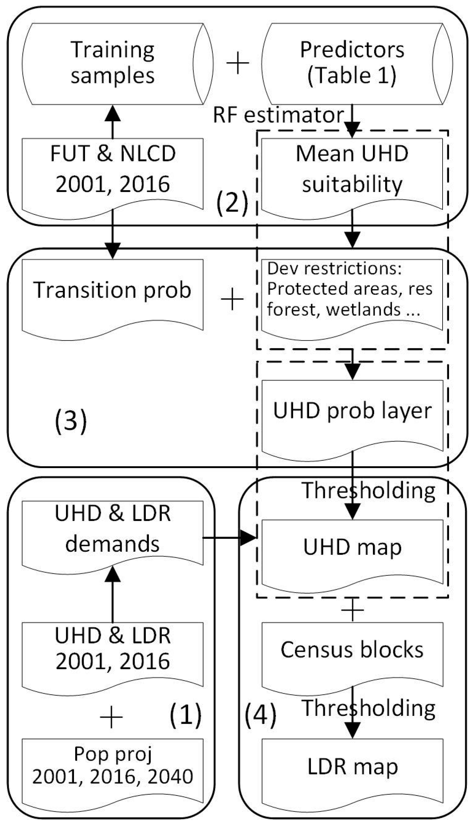
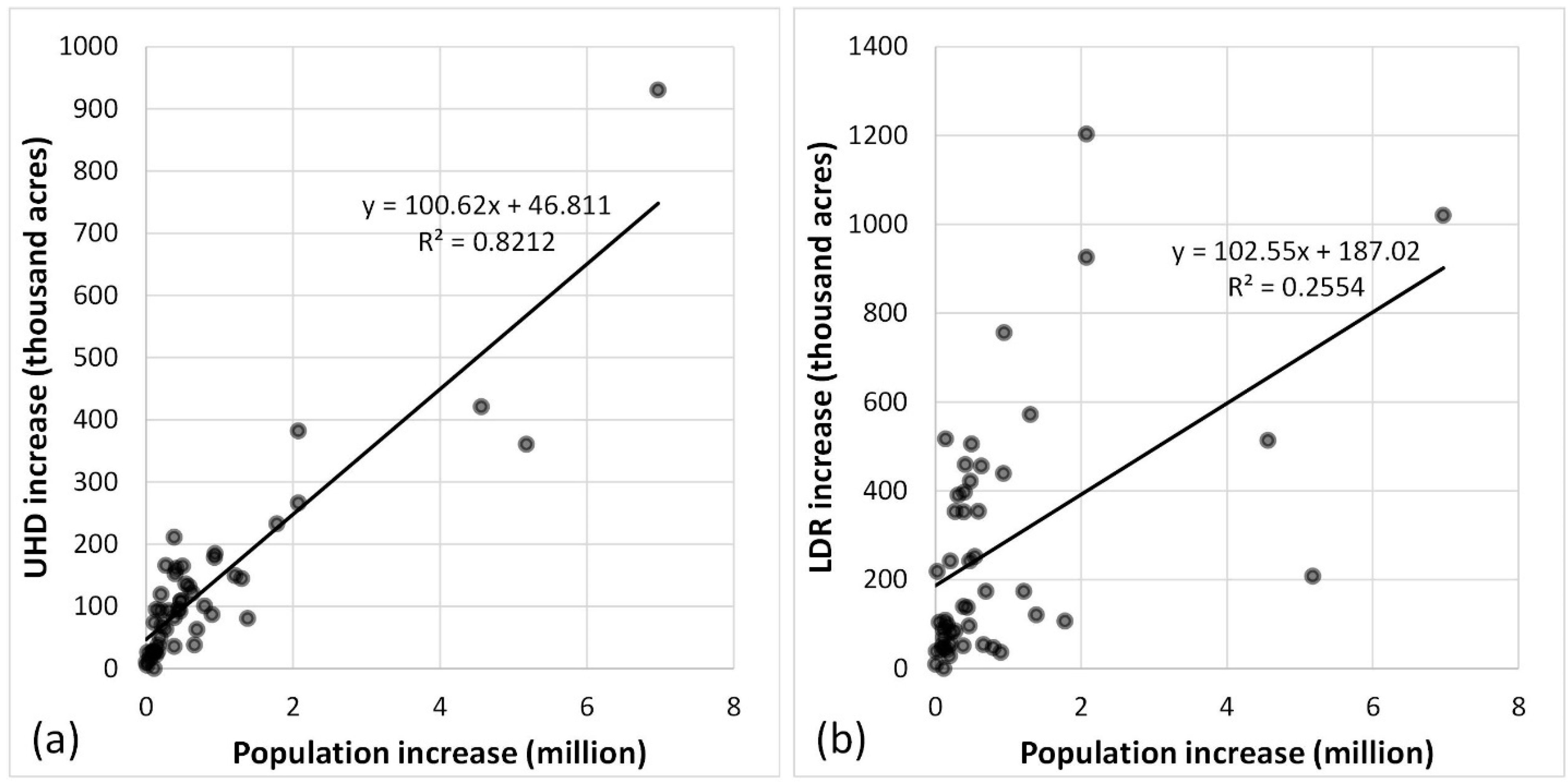
2.1. Projecting Urban Land Demands

In the BAU scenario, development, driven by existing land-use policies and consumer preferences, remains on the same trajectory as that from 2001 to 2016, as documented in Farms Under Threat: The State of the States [24]. For each county, we estimated UHD demand in 2040 (devDemanduhd) as:
d e v D e m a n d u h d = u h d I n c R a t e 2001 2016 24 a d j F a c t o r
where uhdIncRate2001–2016 is the average annual UHD increase in a county from 2001 to 2016 (i.e., total UHD increment divided by 15), adjFactor is the state-level adjusting factor that is used for all counties within a state (see below), and the number 24 refers to the number of years between 2016 and 2040. We used a population-change-driven adjusting factor to reflect projected changes in the rate of UHD development because (1) population increase is a good indicator of high-density urban development (e.g., more buildings are needed to house a growing population) (Figure 2a), and (2) other indicators such as gross domestic product (GDP) are not available at scales fine enough. We calculated the adjusting factor as:
a d j F a c t o r = 1 + r     0.1
where r is the relative change rate of population growth between 2016 and 2040 and 2001–2016:
r = ( p o p I n c R a t e 2016 2040 p o p I n c R a t e 2001 2016 ) / a b s ( p o p I n c R a t e 2001 2016 )
where popIncRate is the average annual population increase (i.e., total population growth during a period divided by the number of years). Population estimates for the years 2001 and 2016 were from the U.S. Census Bureau [45,46], and the state-level population projections are from the Weldon Cooper Center for Public Service, University of Virginia (see details in: https://demographics.coopercenter.org/national-population-projections/, accessed on 15 March 2022). Because both datasets use the population census as reference, we assumed the estimates and projections were consistent and compatible across states and time.
Given the lack of county-level population projections, we calibrated the adjusting factor by state. This procedure of UHD demand estimation reflects the projected change in population growth rate, but it is also designed to not substantially over- or under-estimate future UHD needs. For example, if a state is projected to see 50% faster population growth in 2016–2040 than it did in 2001–2016, the UHD conversion rate would increase by 5%. As a result, the adjustment factor ranges from 0.8 to 1.1 for all states except for West Virginia, which has the largest projected decline in population growth rate (adjustment factor is 0.54).
Finally, we divided UHD demand into two components—LDR-to-UHD and non-LDR-to-UHD—so that future UHD development would occur on LDR at an appropriate rate. Because LDR is usually near existing UHD, it is more likely to be urbanized than non-LDR land uses. Assuming that the proportion of UHD development on LDR (compared to the total UHD development) remains unchanged from 2001 to 2016 and 2016 to 2040, the amount of future LDR-to-UHD conversion was estimated as:
d e v D e m a n d l d r 2 u h d = d e v D e m a n d u h d     p r o p l d r 2 u h d
where propldr2uhd is the proportion of UHD development on LDR from 2001 to 2016. Subsequently, the amount of non-LDR-to-UHD conversion was calculated as devDemanduhddevDemandldr2uhd.
We used a similar method to estimate future LDR demand per county:
d e v D e m a n d l d r = l d r I n c R a t e 2001 2016 24
where ldrIncRate2001–2016 is the average annual LDR increase in a county from 2001 to 2016 (i.e., total LDR increment divided by 15). However, we did not apply a population-driven adjusting factor for LDR demand estimation because past LDR increases were found to have a weak relationship with population change (Figure 2b).

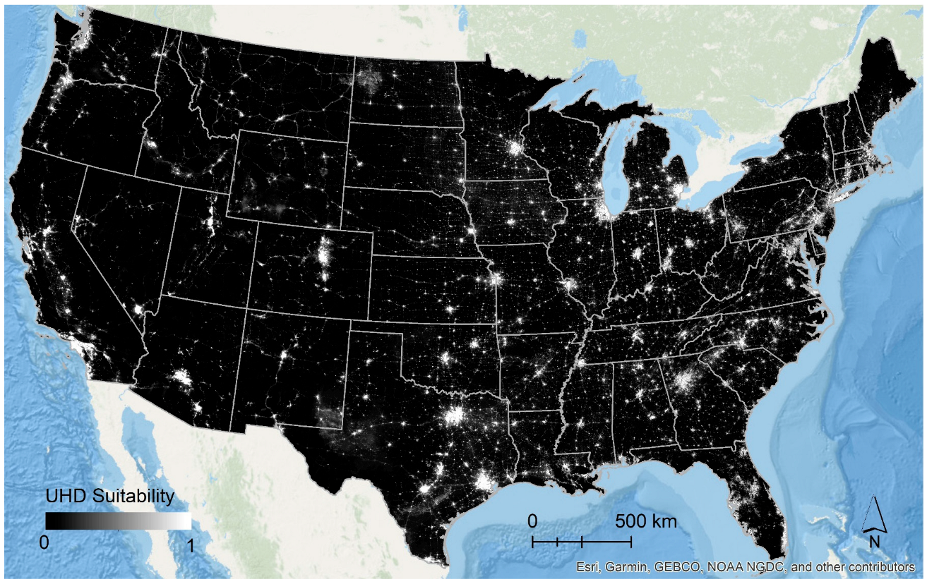
2.2. Creating Development Suitability Layers

We estimated development suitability for each pixel within a county on a scale of 0 to 1 (higher values imply an area more suitable for development), with the potential for a location to be urbanized as defined by a set of spatial and socioeconomic determinants (Table 1). Predictor variables included terrain, relationships to existing urban areas, transportation networks, water resources, other land resources (e.g., protected natural resources), the urban fraction within a pre-defined buffer, land value, and nighttime light intensity (to account for scale-dependent effects of urban development, e.g., urban development can be more likely to occur around large cities for some counties).
We built the UHD suitability layer from these estimators by employing random forest classifiers [47]. The computation of UHD suitability layers was conducted per county. For each county, UHD and non-UHD training samples were randomly stratified from FUT and NLCD 2016 layers. We tested a series of sample sizes (from 50 to 1000 for each class, with an increment of 50) for classifier training. While too dense a sampling scheme can result in the problem of over-fitting the model, too few samples can exaggerate projections. After testing, we found reasonable results (based on visual inspection) were achieved using 400 samples (200 for each class) per county. County-specific random forest classifiers trained from stratified samples and predictor variables were then used to calculate UHD suitability layers. The county-level suitability layers were then mosaicked to create a nationwide map.
Since sample size and location are critical to image classification, as well as to estimate suitability in this study, we repeated the procedure of sample stratification and suitability calculation 100 times. As a result, we created 100 nationwide suitability layers, which were then averaged to generate the mean suitability layer (see Figure 3 for an overview of UHD suitability). This final UHD suitability layer was later used in the steps of estimating development probability and spatial allocation.
Table 1. Socioeconomic and physical variables used to estimate urban development suitability.
Variable Name Spatial ResolutionYear of DataData Sources
Nighttime light intensity500 m2016NOAA NPP/VIIRS
Land value480 m2010[48]
Elevation30 m2000NASS Shuttle Radar Topography Mission
Slope30 m2000
Distance to existing urban boundary 30 m2016FUT2016 and NLCD2016
Distance to primary roads 30 m2016TIGER: US Census Roads
Distance to secondary roads 30 m2016
Distance to water bodies 30 m2016NLCD2016
Size of the closest urban cluster30 m2016FUT2016
Urban fraction within a 1 km ∗ 1 km buffer1 km2016NLCD2016
Distance to forest30 m2016NLCD2016
Distance to protected ag land30 m2016AFT PALD
Distance to protected areas30 m2019PAD-US

2.3. Development Restriction Layers

We assumed certain land uses are unlikely to be urbanized. These areas were removed from the suitability layer before conducting spatial allocation. In this study, development restrictions included existing UHD, federal lands, protected agricultural lands, land in the Protected Areas Database of the U.S. (USGS PAD-US v.2.1), wetlands (only for UHD allocation), and water bodies. The extent of UHD and federal lands were derived from FUT 2016 [24]. Wetlands and water bodies were extracted from NLCD 2016 [49]. The protected agricultural lands dataset (PALD) and PAD-US were from AFT (https://farmlandinfo.org/statistics/pald/, accessed on 15 March 2022) and USGS [50], respectively.
In addition to these areas, mature forestlands within residential areas (urban trees) tend to remain unchanged, given their importance to the urban environment (e.g., reduced urban heat island, ecological and aesthetic values, etc. [51,52,53] (Figure 4). However, residential forestlands are usually classified as LDR in FUT layers, since NLCD 2016 often did not classify them as developed land use. They are also close to UHD, making them likely to receive high suitability values and so are erroneously selected as areas for new UHD conversion. To reserve these LDR areas, we developed a set of rules to identify them using a random forest classifier. We first calculated the proportion of each U.S. census block that was in LDR and other land cover/use classes (derived from FUT and NLCD layers). We then calculated the maximum vegetation greenness in each census block for the years 2001 and 2016. To calculate the vegetation greenness of a block, we first computed a layer of yearly maximum NDVI from all available Landsat images within a year (i.e., 2001 and 2016), which were then aggregated as the mean value of all pixels within the block. Blocks with and without LDR-to-UHD conversion during the period of 2001–2016 were then marked and used as reference to train state-wise random forest classifiers. Predictors included vegetation greenness and land use types and densities for the year 2001. The trained classifiers were later applied to 2016 predictors to predict LDR blocks likely to remain stable from 2016 to 2040. The detected stable LDR blocks were subsequently used as an additional restriction layer for the 2040 UHD projection.

2.4. Creating Development Probability Layers

Development probability is defined as the product of suitability and the historical land use conversion rate (transition probability). We calculated the transition probability statistics at the county level based upon the actual conversion rate of each non-urban land use to urban use between 2001 and 2016 using FUT and NLCD layers. For each county, we calculated the conversion to UHD for each land use in proportion to its total area from 2001 to 2016, including LDR, cultivated lands, forest, herbaceous, wetlands, bare land, and water bodies. Because LDR is an integrated class that covers all other land uses except for UHD, we further calculated the transition probability of each land use within LDR.
The calculation of transition probabilities for each county was conducted only within the peri- to urban areas, as defined by nighttime light brightness greater than 1. The reasons for this design are twofold. First, the area of land uses can vary substantially within a county (e.g., some midwestern counties are dominated by croplands), which could lead to distortions in transition probability if all land uses within the target county are counted. In fact, land uses remote from urban areas tend to remain unurbanized and should have low transition probability. Second, artificial nighttime lights were used to delineate urban and peri-urban boundaries because they have good correlations with human activities, including the extent of urban development [54,55,56]. The brightness threshold of 1 was used to cover the majority of 2016 LDR and UHD extent and remove possible background noise (i.e., lower brightness value for unlit areas due to systematic errors).

2.5. UHD and LDR Projections

After removing development restriction areas (Section 2.3) from the probability layer (Section 2.4), we projected the location of future UHD development using a pixel-based thresholding method. The projections of LDR-to-UHD and non-LDR-to-UHD were conducted separately due to the unique characteristics of LDR compared with other non-LDR land uses. After UHD allocation, the location of LDR development was estimated using a census block-based thresholding method to maintain consistency with the previous FUT approach and datasets. All projections were county-stratified and subsequently mosaiced to nationwide maps.

2.5.1. Allocation of UHD Development

We first estimated where LDR will be converted to UHD. Spatial allocation was applied based on pixel values and urban development demand from LDR (Section 2.1), i.e., we estimated that locations with higher probability values will be urbanized earlier than low-value pixels. A series of thresholds (from 0 to 1 with a step of 0.002) were used to segment the probability layer until the amount of LDR to UHD conversion was met, which resulted in a binary map showing whether an LDR pixel is projected to be developed or not. For each block with LDR in 2016, the maximum conversion to UHD proportion was set as the 75th percentile of the observed 2001–2016 rate of all LDR blocks with LDR-to-UHD conversion within the county. This spatial allocation of LDR-to-UHD conversion was constrained to the 2016 LDR extent.
A similar approach was used to allocate non-LDR-to-UHD conversion, but the projection was conducted within the 2016 non-LDR extent. The two binary projections (i.e., LDR-to-UHD and non-LDR-to-UHD) were then combined to generate a complete map of UHD projections.

2.5.2. Allocation of LDR Development

To be consistent with the 2001 and 2016 FUT layers, LDR projections were conducted at the U.S. Census block level. After allocating UHD locations, we calculated block-level LDR probabilities as the median value of UHD suitability for the remaining undeveloped and available land within census blocks. That is, we excluded existing UHD, LDR, restriction areas, and projected UHD and then calculated the suitability for the remaining block area to identify the location’s likelihood for LDR growth. Finally, we implemented a probability layer-based thresholding method to predict specific locations where LDR development is most likely to occur from 2016 to 2040. Like UHD projections, the thresholding method tested a series of thresholds per county until the LDR demand was met, with the amount of demand allocated to the most probable remaining blocks. All county-wide projections were finally mosaiced to a nationwide map.

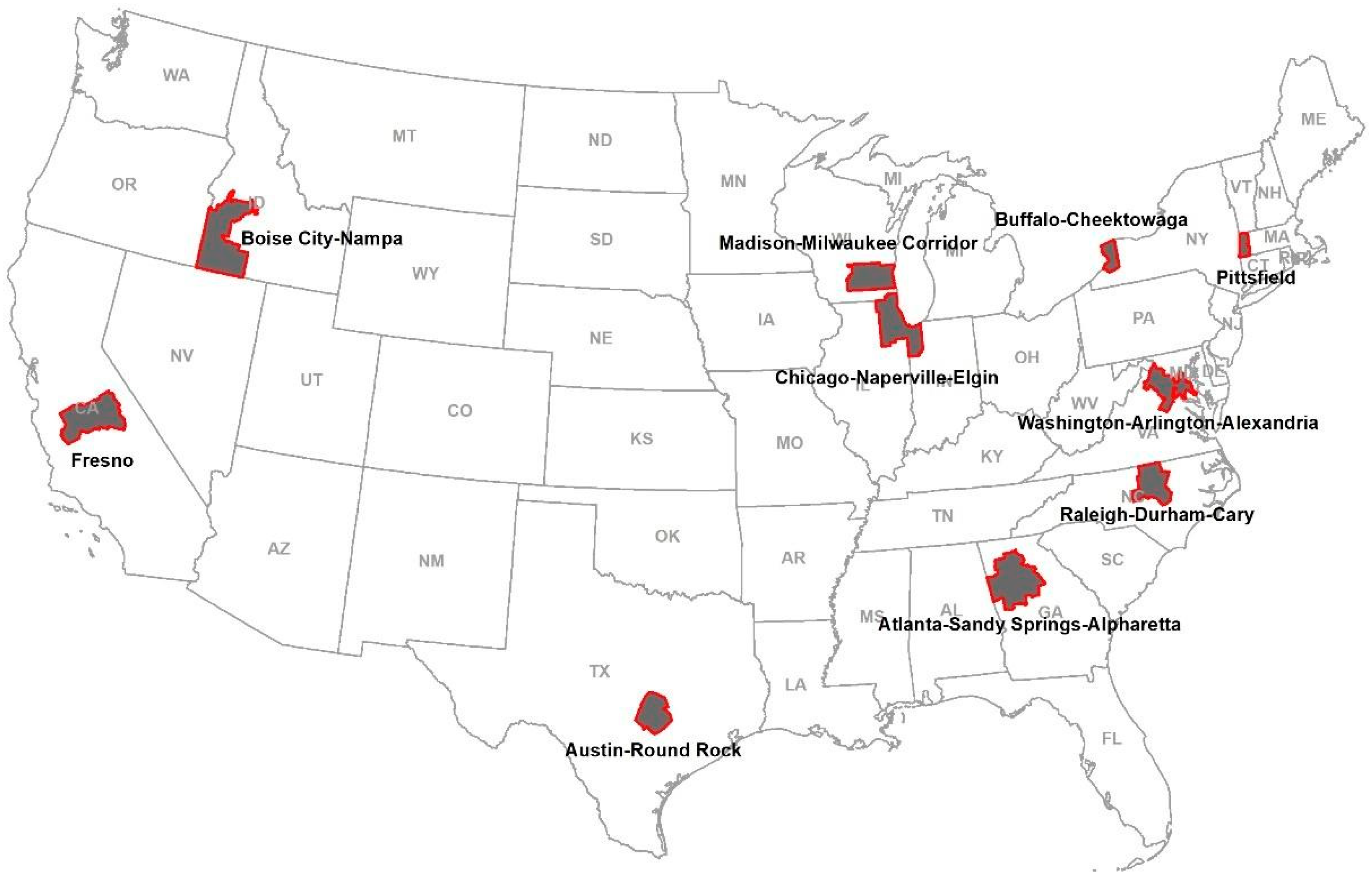
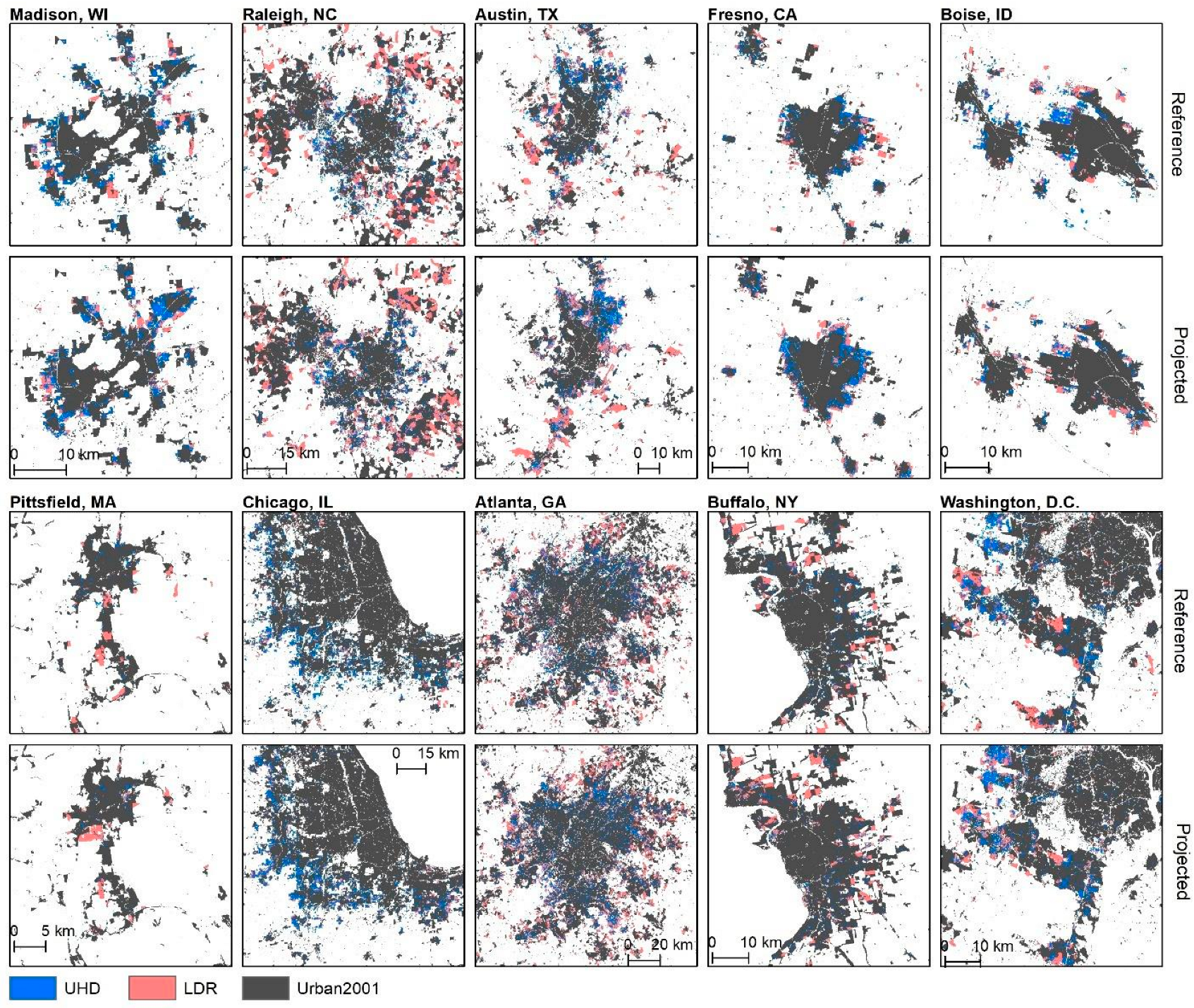
2.6. Model Validation

We first evaluated our projected UHD and LDR maps through discussions and visual evaluation, including by AFT’s regional experts across the country. More particularly, we visually assessed the location, size, and pattern of projected urban clusters based on high-resolution aerial photography, thematic land use maps, and our knowledge of local to regional urban environments. While this visual assessment was able to inform our understanding of the reliability and robustness of our models and projections, quantitative evaluation of the 2040 projections was not possible due to the lack of (future) reference data.
Thus, to quantitatively evaluate our model performance, we compared projected urban development with actual growth for the period 2001 to 2016. Using 2001 as the baseline year, we first projected UHD and LDR growth between 2001 and 2016. This projected urban growth was then compared with reference urban growth observed by FUT in its 2001 and 2016 layers.
Ten cities/metropolitan areas were selected across the country to conduct pixel-wise site-specific locational accuracy assessments (Figure 5). They were selected to represent diverse biophysical and socioeconomic conditions of cities across the country and to target locations with which we were familiar. For each city/metropolitan area, we randomly selected 1000 30 m locations (500 each for change and non-change categories) and calculated accuracy metrics of overall accuracy (OA) and F1 score [57]. The stable UHD extent was removed from the non-change class, as it remains unchanged after being built. Including it in the assessment would artificially increase the apparent reliability of our models.
O A = T h e   n u m b e r   o f   c o r r e c t   c l a s s i f i c a t i o n T o t a l   n u m b e r
F 1 = 2     U A     P A U A + P A
where UA and PA refer to user’s accuracy and producer’s accuracy of the UHD/LDR class, respectively.

3. Results

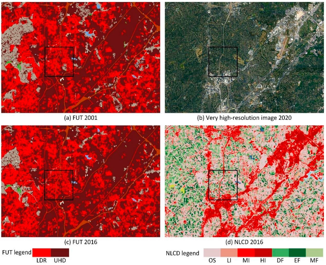
3.1. Map and Model Evaluation for the Period 2001–2016

Running our models for the year 2016 resulted in similar patterns of urban development as compared with FUT-derived reference maps (Figure 6). Quantitatively, our modeling framework predicted UHD growth with a reasonable overall accuracy of 67.1% and an F1 score of 0.51 (Table 2). In general, the accuracies of UHD projection vary across metropolitan statistical areas (MSAs), which were often the unit of modeling. The greatest accuracies were achieved for Boise City, ID; Washington DC; Austin, TX; and Rock and Chicago, IL regions, with accuracies upwards of 70% and F1 scores close to or higher than 0.6. In contrast, accuracies were the lowest for the Pittsfield, MA and Buffalo, NY areas (56–57%), with F1 scores only slightly above 0.2.
The estimation of LDR development was less reliable compared with UHD but still yielded an overall accuracy over 60%. Given the variety of land use compositions within modeling regions, a high UHD estimation for a city/metropolitan area is not an assurance of high accuracy for its LDR projection. For example, Atlanta–Sandy Springs–Alpharetta has the highest LDR projection accuracy (F1 score of 0.57) but is middle-of-the-road for UHD projection accuracy. The lowest LDR accuracies were achieved in Fresno and the Madison–Milwaukee Corridor (F1 scores of 0.12 and 0.25, respectively).
Note, however, that these results reflect the accuracy of UHD and LDR growth, and not their total extent. Estimating growth (a dynamic land-use class) is more difficult than estimating total extent (where most land is static) but gives a better indication of the model’s performance in estimating agricultural land conversion, which is our output of interest. Given (1) the complexity of driving forces of urban development, (2) limited data availability for some variables needed to predict UHD and LDR (e.g., farm size), and (3) the inherent uncertainty in making future predictions [34,38,43], the achieved accuracies should be considered both sufficient and appropriate for making future projections to inform land conservation and prioritization. For reference, commonly acceptable accuracies for the historic detection of dynamic, remotely sensed land cover change classes are often between 60 and 70% [58,59]. Thus, achieving a similar level of overall accuracy for the prediction of change should meet or exceed performance requirements for most applications of these data.

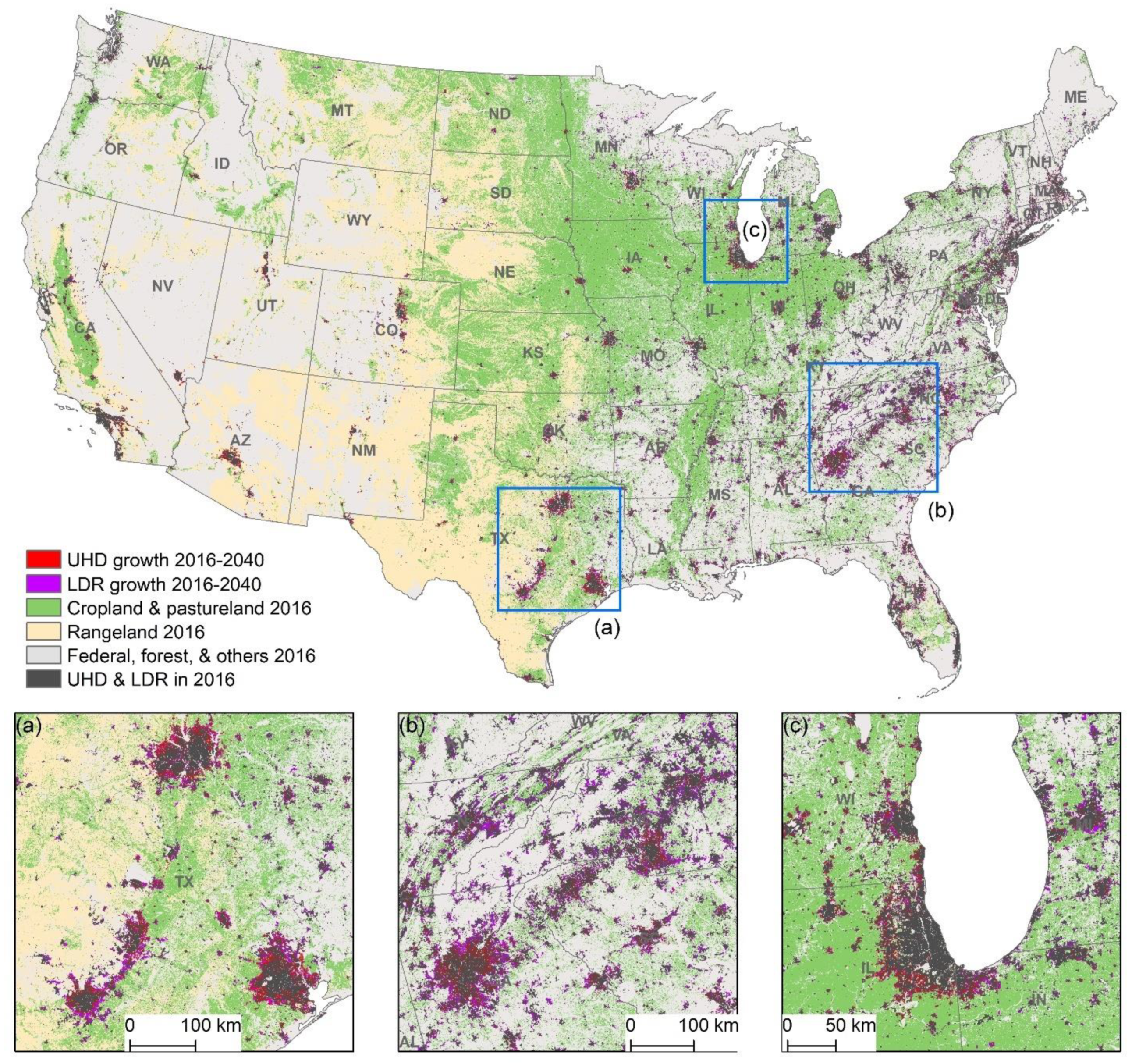
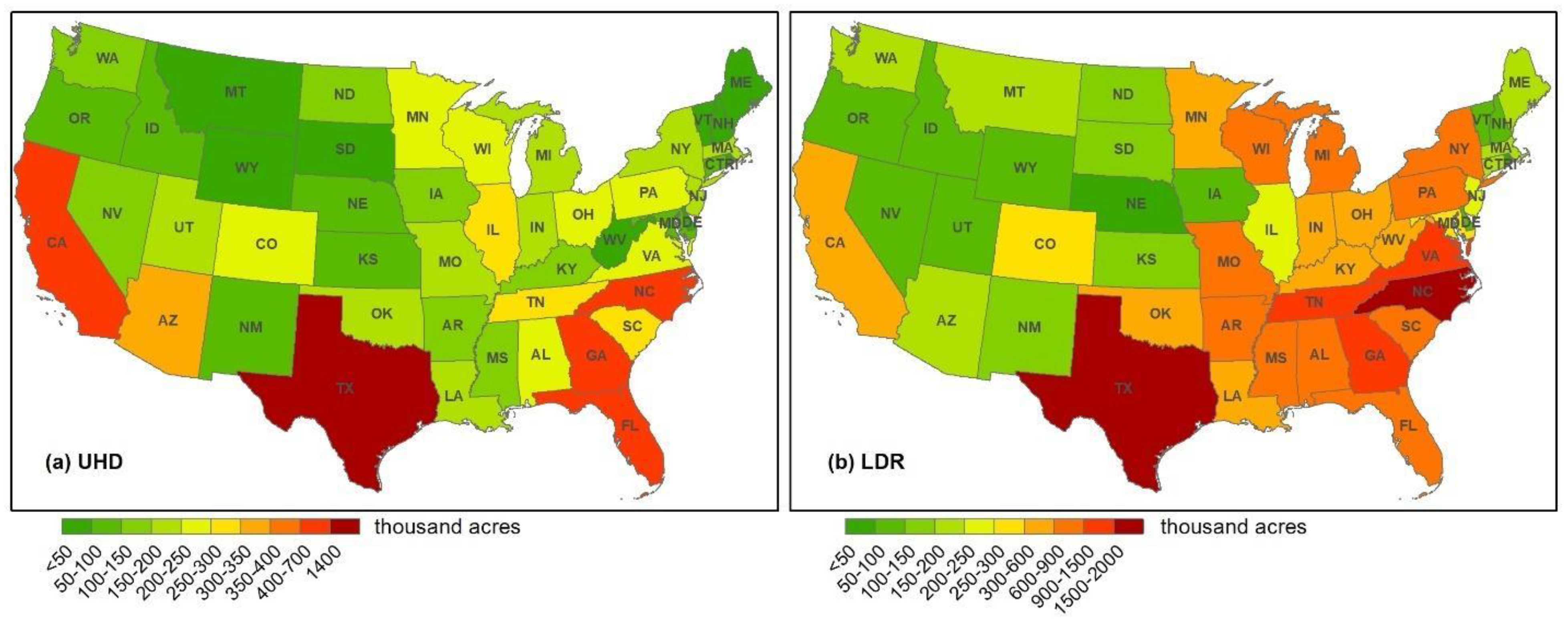
3.2. Spatial Patterns of Projected Urban Development by 2040

The 2040 UHD and LDR development in Figure 7 shows that our proposed model provides reasonable projected urbanization patterns. Our maps show that future urban development will primarily occur in suburban to peri-urban areas where developable lands are available and close to existing low- to high-density built-up areas and transportation networks.
Our projections see diverse local to nationwide urban growth by 2040. If urban development continues at the same pace as that in 2001–2016, our modeling shows an additional 9.5 million acres of UHD development, with 6.2 million occurring on agricultural land nationwide. Notable UHD increases are projected to occur especially in the Southeast, Texas, and California (Figure 8a). Despite being highly urbanized already, several metropolitan areas in these states would continue to expand, such as Riverside, CA; Dallas–Fort Worth, TX; Houston, TX; Austin, TX; Orlando, FL; Atlanta, GA; and Raleigh, NC.
Arizona, Illinois, Tennessee, and South Carolina would also see increases of 250–350 thousand acres of UHD. Metropolitan areas such as Phoenix–Mesa–Chandler, AZ; Chicago, IL; Nashville, TN; and Greenville, SC would experience the largest UHD gains in these states. In addition, we found several cities/metropolitan areas with sizeable UHD expansion in the Midwest and eastern U.S., including Minneapolis–St. Paul–Bloomington, MN–WI; Milwaukee–Waukesha, WI; Columbus, OH; and Washington–Arlington–Alexandria, DC–VA–MD. With the exceptions of California and Arizona, most other western states showed relatively small UHD increases, ranging from <50 to 250 thousand acres.
Accompanying the high-density urban development, our projections also show an additional 21.1 million acres of land that would be converted to LDR use. Compared with UHD, LDR projections show a higher contrast between the western and eastern U.S., with much lower rates of LDR conversion in the west (Figure 8b). Texas and North Carolina show the most LDR development, with increases of >1.5 million acres, followed by Georgia, Tennessee, and Virginia, with 0.9–1.5 million acres, while the Midwest (Minnesota, Wisconsin, Michigan, and Missouri) and some southeast states (South Carolina, Alabama, Mississippi, and Florida) show 0.3–0.9 million acres of LDR conversion.

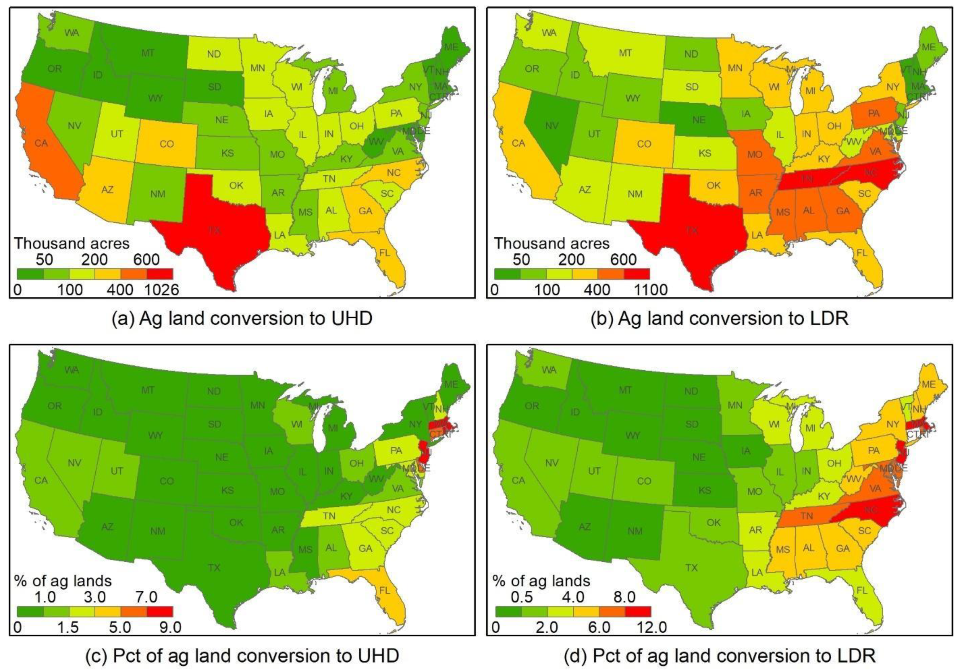
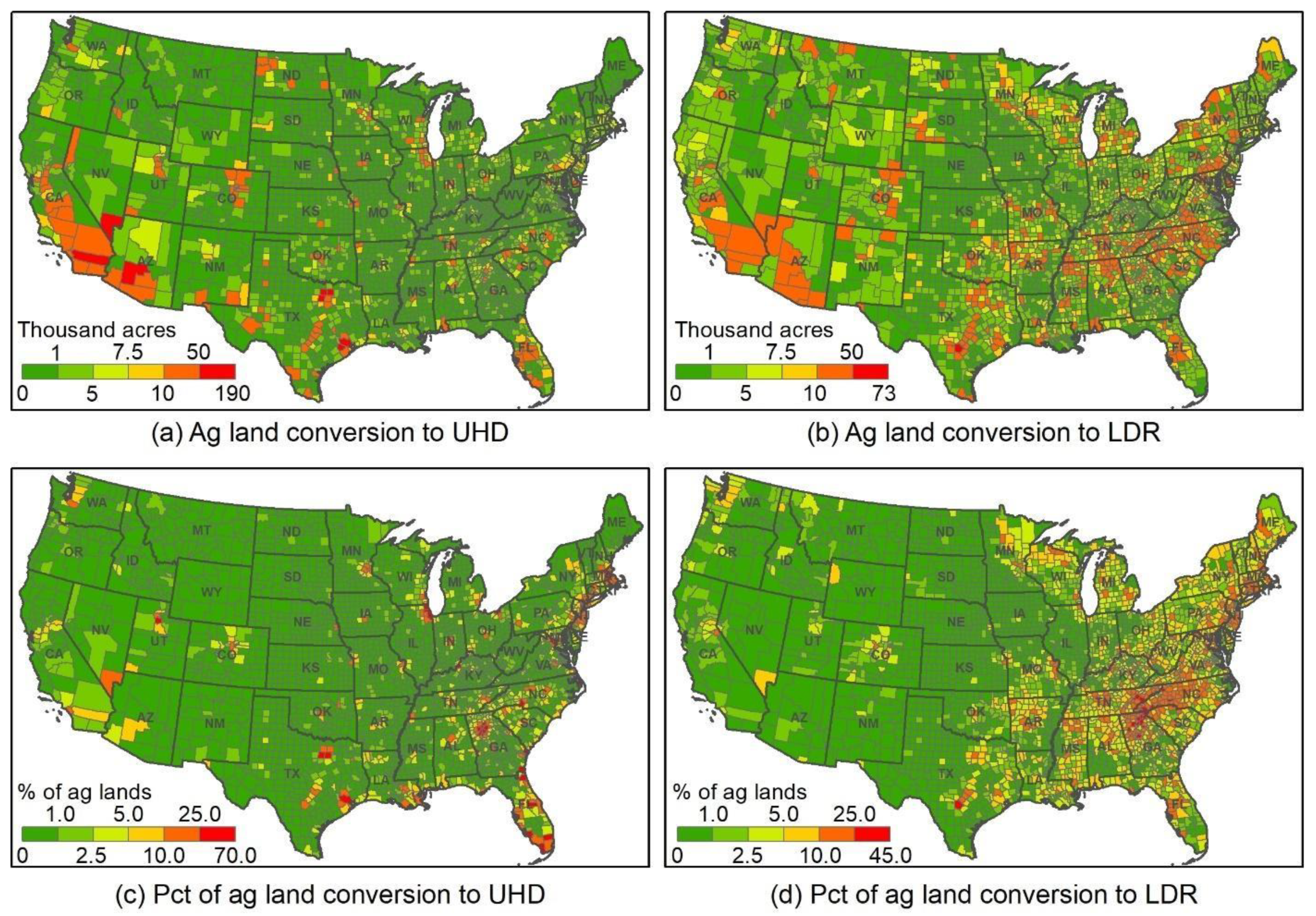
3.3. Farmland under Threat by Urbanization

If urban development continues at the same pace as it did from 2001 to 2016, our projection shows that 18.2 million additional acres of farmland will be lost, fragmented, or compromised by 2040. Of these areas, 6.2 million (34%) will be converted to UHD development, and 12 million (66%) will be vitiated through conversion to LDR land use.
Spatially, agricultural land conversion is particularly concentrated in the Southeast, where six states (North Carolina, Tennessee, Georgia, Florida, Alabama, and Mississippi) would convert between 500,000 to over a million acres by 2040 (Figure 9a,b and Table S1). Texas alone would see over 2 million acres of agricultural lands converted if its cities continue to grow at the existing pace. A cluster of smaller states in the Northeast—New Jersey, Connecticut, Massachusetts, Rhode Island, and Delaware—would see over 10% of their agricultural land lost or fragmented, severely threatening their local food supply and farm economies (Figure 9c,d and Table S2). The state of North Carolina stands out with 11.6% of its agricultural land—nearly 1.2 million acres—projected to be converted to UHD and LDR uses.
Particular hotspots of conversion are even more apparent at the level of counties and metropolitan areas (Figure 10). Shockingly, ten different counties in Georgia would see over 40% of their agricultural land converted (to UHD and LDR) as the Atlanta megalopolis expands. Three Texas counties—Tarrant, Harris, and Dallas—would convert 39–62% of their agricultural land, and in total would lose or fragment over 250,000 acres of agricultural lands. Five North Carolina counties would see more than 35% of their agricultural lands converted. Additionally, at the top of the list, over 70% of agricultural lands in Broomfield County, Colorado will likely be turned over to more developed uses. Beyond these top-ranked counties, it is striking to see how widespread the conversion of agricultural lands will be in the next 20 years under the BAU scenario. Across the country, 2159 counties—nearly two-thirds of the total number of counties in the U.S.—will have at least 1000 acres of conversion. Additionally, among counties that will see over 100 acres of conversion, 445 of them will see at least 10% of their agricultural land lost, fragmented, or compromised.

4. Discussion

4.1. Impacts on Local to National Food Security

Among all possible urbanization-induced agricultural land losses, we found nearly 50% (9.0 million acres) will occur on nationally significant land, defined as the most productive, versatile, and resilient lands (See Text S1 for the definition of nationally significant land). These lands are of particular value to the continued production of food as the warming climate makes it harder to farm and our growing population puts ever higher demands on the food system. Although two-thirds of the projected conversion (i.e., that to LDR) may not permanently replace agricultural lands with uncultivable impervious surfaces, it can still greatly increase the risk of permanent conversion and drastically undermine family farmers, the agricultural land base, and our food security. Meanwhile, to make up for agricultural land losses, cultivation would likely shift to land with lower productivity, which would put even more pressure on already overtaxed water, soil, and biodiversity [60,61].
This substantial loss of significant farmland is especially concerning for metropolitan areas where urban extent will continue to expand rapidly on limited agricultural lands, such as Phoenix, AZ; Riverside–San Bernardino–Ontario, CA; Dallas–Fort Worth–Arlington, TX; and most metropolises on the east coast. The projected continued growth of metropolises could possibly threaten the variety, quality, and security of food production and supply in the U.S. For instance, metropolitan counties and adjacent areas supply nearly 60% of the market value of U.S. farm production and they play important roles from local to national food security [17]. These counties supply 91% of domestically sourced fruits, tree nuts, and berries; 77% of vegetables and melons; 68% of dairy; and 55% of eggs and poultry [17]. Farms in metropolitan counties often supply local and regional markets, making up 81% of the food sold directly to consumers; 76% of community-supported farms; and 74% of farms selling directly to retail outlets [17,24]. It is important to note that fruits and vegetables often require unique soils and microclimates, access to water and labor, an existing infrastructure that has been built up over time (e.g., farm equipment, storage, processing, and packing facilities, etc.), and markets to support production and sales [62]. The difficulty in moving the production of these high-value crops elsewhere has likely kept producers from expanding production, even though domestic demand for fruit and vegetables continuously increases [17,63].

4.2. Policy Implications

To meet the twin goals of sustainable urban development and food production, it will be imperative for planners, policymakers, and concerned citizens to guide future urban expansion toward more condensed forms and prioritize the protection of agricultural land before it is lost. Encouraging compact, public transport-oriented urban forms could help contain the expansion of urban areas, thereby preserving agricultural lands in peri-urban and suburban areas [64]. In addition to urban development policies that could reduce development on agricultural lands, a comprehensive national strategy is needed. Such approaches could include, for example, (1) increasing federal investments in agricultural land protection through the USDA Agricultural Conservation Easement Program—Agricultural Land Easement, (2) supporting programs that provide spatially explicit information to help monitor changes in U.S. agricultural resources, and (3) enhancing federal agricultural land protection platforms to more effectively address the interconnected threats to farmland from development [24]. At the state level, multiple policy approaches should be used and enhanced, depending on the nature and extent of the threat, its underlying causes, each state’s policy framework, and public support. Actions available to individual states include (1) mapping and analyzing detailed conditions and trends of agricultural resources, (2) strengthening and/or adopting a suite of coordinated policies to protect farmland, (3) supporting farm viability and access to land for a new generation of farmers, and (4) establishing a public-policy framework to support agricultural economic development and to protect farmland for current and future generations [17].
The effectiveness of urban planning and agricultural land protection strategies depends on many factors, including the willpower of policymakers, geographic contexts, and local to regional demographic, economic, and societal conditions. If we can reduce UHD and LDR expansion by 25% and 50%, respectively, over the next 20 years (see definition of the better-built-cities scenario in Table S3 and more scenario description details in [65]), 7.5 million fewer acres of agricultural lands would be lost or compromised relative to the BAU scenario (Table S1). This is the equivalent of saving an area roughly equivalent to the state of Maryland. Across the nation, 42% less of our nationally significant farmland would be converted in such a scenario. Some states stand to particularly benefit from this smart planning: in New Mexico, for example, only one-third as many acres of nationally significant farmlands would be converted, and in just four states (Texas, North Carolina, Tennessee, and Ohio), we could save over a million acres of our nationally significant farmland.
Alternatively, if sprawling exurban development accelerates over the next 20 years (for example, adding 50% more LDR to the BAU scenario, as captured by the runaway-sprawl scenario in Table S3, with more scenario description details in [65]), we estimate that 6 million more acres of agricultural lands would be lost or degraded—an area roughly the size of New Hampshire. In such a future with unfettered expansion of large-lot housing, over 12 million acres of nationally significant land would be lost or compromised by 2040. Compared with BAU, an additional half million acres would be converted in both Texas and North Carolina, with Tennessee, Georgia, and Virginia close behind (Table S1). Meanwhile, Connecticut, North Carolina, New Jersey, and Delaware would see an additional 4–5% of their farmland converted (Table S2). As a result, Connecticut and New Jersey would both see over 20% of their remaining farmland converted by 2040. While conversion increases 33% nationwide in this runaway sprawl scenario compared with BAU, Vermont would see nearly 50% more farmland conversion, and Montana, West Virginia, Mississippi, and Michigan would experience 44–46% more.
Given that development is just one of the many threats to the nation’s agricultural lands, more cooperative efforts should be made by urban residents, farmers, planners, and policymakers to mitigate the risks that can take agricultural lands out of production. Several other factors that should be simultaneously considered might include climate change (e.g., sea level rise and droughts), extreme weather, and demographic and land ownership changes. Collectively, these threats to our agricultural lands are likely to strain our future food production systems. By studying the likely patterns, processes, and impacts of these threats to our landscapes, society, and the environment, we stand a better chance of navigating their associated challenges and improving our agricultural systems and their resiliency.

5. Conclusions

To evaluate possible agricultural land losses to future urban development in the U.S., we developed a spatially explicit machine learning method to forecast urban expansion by 2040 under a business-as-usual scenario. The analysis of our projected map shows that highly developed urban areas would increase by 9.5 million acres (as compared with the baseline year of 2016) if urban development continues at the same pace, with another 21.1 million to be converted to low-density residential uses. This increase would collectively result in 18.2 million acres of agricultural land lost and fragmented. Considerable agricultural land loss would take place particularly in the southern states (e.g., Texas, California, and the southeast coast) and metropolitan areas that play important roles in community, regional, and nationwide food supply. Since urbanization is not just a local issue, our analysis further emphasizes the necessity of cooperative efforts from local to federal policymakers to relieve land use competitions between urban and agricultural systems.

Supplementary Materials

The following supporting information can be downloaded at: https://www.mdpi.com/article/10.3390/land12030574/s1. Text S1. Nationally significant land; Table S1. Per-state agricultural lands projected to be converted to highly developed urban and low-density residential use by 2040. Ag2UHD: agricultural lands converted to highly developed urban use; Ag2LDR: agricultural lands converted to low-density residential use; LDR2UHD: low-density residential land converted to highly developed urban use; Ag2Urban: agricultural lands converted to either highly developed urban or low-density residential use (Ag2UHD + Ag2LDR). States are ranked by Ag2Urban. Units in thousand acres; Table S2. States with the greatest proportion of agricultural land projected to be converted to highly developed urban and low-density residential uses by 2040. Units in percent of total agricultural land; Table S3. Modeling assumptions for the business-as-usual, runaway-sprawl, and better-built-cities scenarios.

Author Contributions

Conceptualization, Y.X., M.H. and T.J.L.; methodology, Y.X. and M.H.; software, Y.X.; validation, Y.X., M.H., A.S., T.N.-M., J.P.S., S.L. and T.J.L.; writing—original draft preparation, Y.X.; writing—review and editing, Y.X., M.H., A.S., T.N.-M., J.P.S., S.L. and T.J.L.; visualization, R.M.; funding acquisition, T.J.L. and Y.X. All authors have read and agreed to the published version of the manuscript.

Funding

USDA NRCS from the American Farmland Trust-USDA Natural Resource Contribution Agreements 68-3A75-14-214 and 68-3A75-18-005.

Data Availability Statement

The projected maps in this study are available on request from the corresponding authors. Map visualization is available at http://development2040.farmland.org, accessed on 1 October 2022.

Acknowledgments

The authors would like to thank members of the American Farmland Trust and Conservation Science Partners for supplying data, their feedback and ideas for mapping, and their insights regarding data. We also thank the anonymous reviewers and editors for their helpful comments.

Conflicts of Interest

The authors declare no conflict of interest.

References

  1. Seto, K.C.; Ramankutty, N. Hidden linkages between urbanization and food systems. Science 2016, 352, 943–945. [Google Scholar] [CrossRef]
  2. van Vliet, J. Direct and indirect loss of natural area from urban expansion. Nat. Sustain. 2019, 2, 755–763. [Google Scholar] [CrossRef]
  3. Huang, Q.; Liu, Z.; He, C.; Gou, S.; Bai, Y.; Wang, Y.; Shen, M. The occupation of cropland by global urban expansion from 1992 to 2016 and its implications. Environ. Res. Lett. 2020, 15, 084037. [Google Scholar] [CrossRef] [Green Version]
  4. Seto, K.C.; Fragkias, M.; Güneralp, B.; Reilly, M.K. A Meta-Analysis of Global Urban Land Expansion. PLoS ONE 2011, 6, e23777. [Google Scholar] [CrossRef]
  5. Shi, K.; Chen, Y.; Yu, B.; Xu, T.; Li, L.; Huang, C.; Liu, R.; Chen, Z.; Wu, J. Urban Expansion and Agricultural Land Loss in China: A Multiscale Perspective. Sustainability 2016, 8, 790. [Google Scholar] [CrossRef] [Green Version]
  6. Pandey, B.; Seto, K.C. Urbanization and agricultural land loss in India: Comparing satellite estimates with census data. J. Environ. Manag. 2015, 148, 53–66. [Google Scholar] [CrossRef] [PubMed]
  7. Martellozzo, F.; Ramankutty, N.; Hall, R.; Price, D.; Purdy, B.; Friedl, M. Urbanization and the loss of prime farmland: A case study in the Calgary-Edmonton corridor of Alberta. Reg. Environ. Chang. 2014, 15, 881–893. [Google Scholar] [CrossRef]
  8. Lasisi, M.; Popoola, A.; Adediji, A.; Adedeji, O.; Babalola, K. City expansion and agricultural land loss within the peri-urban area of Osun State, Nigeria. Ghana J. Geogr. 2017, 9, 132–163. [Google Scholar]
  9. Youssef, A.; Sewilam, H.; Khadr, Z. Impact of Urban Sprawl on Agriculture Lands in Greater Cairo. J. Urban Plan. Dev. 2020, 146, 05020027. [Google Scholar] [CrossRef]
  10. Gandharum, L.; Hartono, D.M.; Karsidi, A.; Ahmad, M. Monitoring Urban Expansion and Loss of Agriculture on the North Coast of West Java Province, Indonesia, Using Google Earth Engine and Intensity Analysis. Sci. World J. 2022, 2022, 3123788. [Google Scholar] [CrossRef]
  11. Andrade, J.F.; Cassman, K.G.; Rattalino Edreira, J.I.; Agus, F.; Bala, A.; Deng, N.; Grassini, P. Impact of urbanization trends on production of key staple crops. Ambio 2022, 51, 1158–1167. [Google Scholar] [CrossRef] [PubMed]
  12. Bren D’Amour, C.; Reitsma, F.; Baiocchi, G.; Barthel, S.; Güneralp, B.; Erb, K.-H.; Haberl, H.; Creutzig, F.; Seto, K.C. Future urban land expansion and implications for global croplands. Proc. Natl. Acad. Sci. USA 2017, 114, 8939–8944. [Google Scholar] [CrossRef] [PubMed] [Green Version]
  13. Zhuang, H.; Chen, G.; Yan, Y.; Li, B.; Zeng, L.; Ou, J.; Liu, K.; Liu, X. Simulation of urban land expansion in China at 30 m resolution through 2050 under shared socioeconomic pathways. GIScience Remote Sens. 2022, 59, 1301–1320. [Google Scholar] [CrossRef]
  14. Chen, G.; Li, X.; Liu, X.; Chen, Y.; Liang, X.; Leng, J.; Xu, X.; Liao, W.; Qiu, Y.; Wu, Q.; et al. Global projections of future urban land expansion under shared socioeconomic pathways. Nat. Commun. 2020, 11, 537. [Google Scholar] [CrossRef] [PubMed] [Green Version]
  15. van Vliet, J.; Eitelberg, D.A.; Verburg, P.H. A global analysis of land take in cropland areas and production displacement from urbanization. Glob. Environ. Chang. 2017, 43, 107–115. [Google Scholar] [CrossRef]
  16. FAO. The State of the World’s Land and Water Resources for Food and Agriculture (SOLAW)—Managing Systems at Risk; Earthscan: London, UK; FAO: Rome, Italy, 2011. [Google Scholar]
  17. Sorensen, A.; Freedgood, J.; Dempsey, J.; Theobald, D. Farms Under Threat: The State of America’s Farmland; American Farmland Trust: Washington, DC, USA, 2018. [Google Scholar]
  18. D’Odorico, P.; Carr, J.A.; Laio, F.; Ridolfi, L.; Vandoni, S. Feeding humanity through global food trade. Earth’s Future 2014, 2, 458–469. [Google Scholar] [CrossRef]
  19. Lark, T.J.; Hendricks, N.P.; Smith, A.; Pates, N.; Spawn-Lee, S.A.; Bougie, M.; Booth, E.G.; Kucharik, C.J.; Gibbs, H.K. Environmental outcomes of the US Renewable Fuel Standard. Proc. Natl. Acad. Sci. USA 2022, 119, e2101084119. [Google Scholar] [CrossRef]
  20. Lark, T.J.; Salmon, J.M.; Gibbs, H.K. Cropland expansion outpaces agricultural and biofuel policies in the United States. Environ. Res. Lett. 2015, 10, 044003. [Google Scholar] [CrossRef] [Green Version]
  21. Durán, A.P.; Duffy, J.; Gaston, K.J. Exclusion of agricultural lands in spatial conservation prioritization strategies: Consequences for biodiversity and ecosystem service representation. Proc. R. Soc. B Boil. Sci. 2014, 281, 20141529. [Google Scholar] [CrossRef]
  22. Scherr, S.J.; McNeely, J.A. Biodiversity conservation and agricultural sustainability: Towards a new paradigm of ‘ecoagriculture’ landscapes. Philos. Trans. R. Soc. B Biol. Sci. 2007, 363, 477–494. [Google Scholar] [CrossRef] [Green Version]
  23. Radeloff, V.C.; Helmers, D.P.; Kramer, H.A.; Mockrin, M.H.; Alexandre, P.M.; Bar-Massada, A.; Butsic, V.; Hawbaker, T.J.; Martinuzzi, S.; Syphard, A.D. Rapid growth of the US wildland-urban interface raises wildfire risk. Proc. Natl. Acad. Sci. USA 2018, 115, 3314–3319. [Google Scholar] [CrossRef] [PubMed] [Green Version]
  24. Freedgood, J.; Hunter, M.; Dempsey, J.; Sorensen, A. Farms Under Threat: The State of the States; American Farmland Trust: Washington, DC, USA, 2020. [Google Scholar]
  25. Lund, S.; Madgavkar, A.; Manyika, J.; Smit, S.; Ellingrud, K.; Meaney, M.; Robinson, O. The Future of Work after COVID-19; McKinsey Global Institute: Washington, DC, USA, 2021; Volume 18, Available online: https://www.voced.edu.au/content/ngv:89731 (accessed on 15 March 2022).
  26. Parker, K.; Horowitz, J.M.; Minkin, R. Americans Are Less Likely than before COVID-19 to Want to Live in Cities, More Likely to Prefer Suburbs. 2021. Available online: https://policycommons.net/artifacts/2047074/americans-are-less-likely-than-before-covid-19-to-want-to-live-in-cities-more-likely-to-prefer-suburbs/2799982/ (accessed on 20 October 2022).
  27. Wadduwage, S. Peri-urban agricultural land vulnerability due to urban sprawl—A multi-criteria spatially-explicit scenario analysis. J. Land Use Sci. 2018, 13, 358–374. [Google Scholar] [CrossRef] [Green Version]
  28. Almeida, C.d.; Gleriani, J.; Castejon, E.F.; Soares-Filho, B.S. Using neural networks and cellular automata for modelling intra-urban land-use dynamics. Int. J. Geogr. Inf. Sci. 2008, 22, 943–963. [Google Scholar] [CrossRef]
  29. Li, X.; Yeh, A.G.-O. Neural-network-based cellular automata for simulating multiple land use changes using GIS. Int. J. Geogr. Inf. Sci. 2002, 16, 323–343. [Google Scholar] [CrossRef]
  30. White, R.; Engelen, G.; Uljee, I. The use of constrained cellular automata for high-resolution modelling of urban land-use dynamics. Environ. Plan. B Plan. Des. 1997, 24, 323–343. [Google Scholar] [CrossRef]
  31. Verburg, P.H.; Soepboer, W.; Veldkamp, A.; Limpiada, R.; Espaldon, V.; Mastura, S.S.A. Modeling the Spatial Dynamics of Regional Land Use: The CLUE-S Model. Environ. Manag. 2002, 30, 391–405. [Google Scholar] [CrossRef]
  32. Sohl, T.L.; Sayler, K.; Drummond, M.A.; Loveland, T.R. The FORE-SCE model: A practical approach for projecting land cover change using scenario-based modeling. J. Land Use Sci. 2007, 2, 103–126. [Google Scholar] [CrossRef]
  33. Van Asselen, S.; Verburg, P.H. Land cover change or land-use intensification: Simulating land system change with a global-scale land change model. Glob. Chang. Biol. 2013, 19, 3648–3667. [Google Scholar] [CrossRef] [PubMed]
  34. Liu, X.; Liang, X.; Li, X.; Xu, X.; Ou, J.; Chen, Y.; Li, S.; Wang, S.; Pei, F. A future land use simulation model (FLUS) for simulating multiple land use scenarios by coupling human and natural effects. Landsc. Urban Plan. 2017, 168, 94–116. [Google Scholar] [CrossRef]
  35. Bierwagen, B.G.; Theobald, D.M.; Pyke, C.R.; Choate, A.; Groth, P.; Thomas, J.V.; Morefield, P. National housing and impervious surface scenarios for integrated climate impact assessments. Proc. Natl. Acad. Sci. USA 2010, 107, 20887–20892. [Google Scholar] [CrossRef] [Green Version]
  36. Radeloff, V.C.; Nelson, E.; Plantinga, A.J.; Lewis, D.J.; Helmers, D.; Lawler, J.; Withey, J.; Beaudry, F.; Martinuzzi, S.; Butsic, V. Economic-based projections of future land use in the conterminous United States under alternative policy scenarios. Ecol. Appl. 2012, 22, 1036–1049. [Google Scholar] [CrossRef] [PubMed] [Green Version]
  37. Sohl, T.L.; Sayler, K.L.; Bouchard, M.A.; Reker, R.R.; Friesz, A.M.; Bennett, S.L.; Sleeter, B.M.; Sleeter, R.R.; Wilson, T.; Soulard, C.; et al. Spatially explicit modeling of 1992–2100 land cover and forest stand age for the conterminous United States. Ecol. Appl. 2014, 24, 1015–1036. [Google Scholar] [CrossRef] [PubMed]
  38. Theobald, D.M. Landscape Patterns of Exurban Growth in the USA from 1980 to 2020. Ecol. Soc. 2005, 10, 32. [Google Scholar] [CrossRef] [Green Version]
  39. West, T.O.; Le Page, Y.; Huang, M.; Wolf, J.; Thomson, A.M. Downscaling global land cover projections from an integrated assessment model for use in regional analyses: Results and evaluation for the US from 2005 to 2095. Environ. Res. Lett. 2014, 9, 064004. [Google Scholar] [CrossRef] [Green Version]
  40. Seto, K.C.; Guneralp, B.; Hutyra, L.R. Global forecasts of urban expansion to 2030 and direct impacts on biodiversity and carbon pools. Proc. Natl. Acad. Sci. USA 2012, 109, 16083–16088. [Google Scholar] [CrossRef] [PubMed] [Green Version]
  41. Strengers, B.; Leemans, R.; Eickhout, B.; de Vries, B.; Bouwman, L. The land-use projections and resulting emissions in the IPCC SRES scenarios scenarios as simulated by the IMAGE 2.2 model. Geojournal 2004, 61, 381–393. [Google Scholar] [CrossRef]
  42. Zhou, Y.; Varquez, A.C.G.; Kanda, M. High-resolution global urban growth projection based on multiple applications of the SLEUTH urban growth model. Sci. Data 2019, 6, 34. [Google Scholar] [CrossRef] [Green Version]
  43. Sohl, T.L.; Wimberly, M.C.; Radeloff, V.C.; Theobald, D.M.; Sleeter, B.M. Divergent projections of future land use in the United States arising from different models and scenarios. Ecol. Model. 2016, 337, 281–297. [Google Scholar] [CrossRef] [Green Version]
  44. CSP. Description of the Approach, Data, and Analytical Methods Used for the Farms Under Threat: State of the States Project; Version 2.0; American Farmland Trust: Truckee, CA, USA, 2020. [Google Scholar]
  45. USCB. USCB: State Intercensal Tables, 2000–2010. 2021. Available online: https://www.census.gov/data/datasets/time-series/demo/popest/intercensal-2000-2010-state.html (accessed on 15 March 2022).
  46. USCB. USCB: State Population Totals and Components of Change, 2010–2019. 2021. Available online: https://www.census.gov/data/tables/time-series/demo/popest/2010s-state-total.html (accessed on 15 March 2022).
  47. Breiman, L. Random forests. Mach. Learn. 2001, 45, 5–32. [Google Scholar] [CrossRef] [Green Version]
  48. Nolte, C. High-resolution land value maps reveal underestimation of conservation costs in the United States. Proc. Natl. Acad. Sci. USA 2020, 117, 29577–29583. [Google Scholar] [CrossRef]
  49. Yang, L.; Jin, S.; Danielson, P.; Homer, C.; Gass, L.; Bender, S.M.; Case, A.; Costello, C.; Dewitz, J.; Fry, J.; et al. A new generation of the United States National Land Cover Database: Requirements, research priorities, design, and implementation strategies. ISPRS J. Photogramm. Remote Sens. 2018, 146, 108–123. [Google Scholar] [CrossRef]
  50. U.S. Geological Survey (USGS) Gap Analysis Project (GAP). Protected Areas Database of the United States (PAD-US) 2.1: U.S. Geological Survey Data Release. 2020. Available online: https://www.sciencebase.gov/catalog/item/5f186a2082cef313ed843257 (accessed on 15 March 2022).
  51. Nowak, D.J.; Crane, D.E.; Stevens, J.C.; Hoehn, R.E.; Walton, J.T.; Bond, J. A Ground-Based Method of Assessing Urban Forest Structure and Ecosystem Services. Arboric. Urban For. 2008, 34, 347–358. [Google Scholar] [CrossRef]
  52. Tyrväinen, L.; Silvennoinen, H.; Kolehmainen, O. Ecological and aesthetic values in urban forest management. Urban For. Urban Green. 2003, 1, 135–149. [Google Scholar] [CrossRef]
  53. Ziter, C.D.; Pedersen, E.J.; Kucharik, C.J.; Turner, M.G. Scale-dependent interactions between tree canopy cover and impervious surfaces reduce daytime urban heat during summer. Proc. Natl. Acad. Sci. USA 2019, 116, 7575–7580. [Google Scholar] [CrossRef] [PubMed] [Green Version]
  54. Elvidge, C.D.; Baugh, K.E.; Kihn, E.A.; Kroehl, H.W.; Davis, E.R.; Davis, C.W. Relation between satellite observed visible-near infrared emissions, population, economic activity and electric power consumption. Int. J. Remote Sens. 1997, 18, 1373–1379. [Google Scholar] [CrossRef]
  55. Sutton, P.C.; Elvidge, C.D.; Ghosh, T. Estimation of gross domestic product at sub-national scales using nighttime satellite imagery. Int. J. Ecol. Econ. Stat. 2007, 8, 5–21. [Google Scholar]
  56. Xie, Y.; Weng, Q.; Fu, P. Temporal variations of artificial nighttime lights and their implications for urbanization in the conterminous United States, 2013–2017. Remote Sens. Environ. 2019, 225, 160–174. [Google Scholar] [CrossRef]
  57. Powers, D.M. Evaluation: From precision, recall and F-measure to ROC, informedness, markedness and correlation. arXiv 2020, arXiv:2010.16061. [Google Scholar]
  58. Foody, G.M. Status of land cover classification accuracy assessment. Remote Sens. Environ. 2002, 80, 185–201. [Google Scholar] [CrossRef]
  59. Stehman, S.V.; Foody, G.M. Key issues in rigorous accuracy assessment of land cover products. Remote Sens. Environ. 2019, 231, 111199. [Google Scholar] [CrossRef]
  60. Lark, T.J.; Spawn, S.A.; Bougie, M.; Gibbs, H.K. Cropland expansion in the United States produces marginal yields at high costs to wildlife. Nat. Commun. 2020, 11, 4295. [Google Scholar] [CrossRef] [PubMed]
  61. Xie, Y.; Lark, T.J. Mapping annual irrigation from Landsat imagery and environmental variables across the conterminous United States. Remote Sens. Environ. 2021, 260, 112445. [Google Scholar] [CrossRef]
  62. Plattner, K.; Perez, A.; Thornsbury, S. Evolving US Fruit Markets and Seasonal Grower Price Patterns; USDA Economic Research Service: Washington, DC, USA, 2014.
  63. White, R.R.; Hall, M.B. Nutritional and greenhouse gas impacts of removing animals from US agriculture. Proc. Natl. Acad. Sci. USA 2017, 114, E10301–E10308. [Google Scholar] [CrossRef] [PubMed]
  64. Daniels, T. When City and Country Collide: Managing Growth in the Metropolitan Fringe; Island Press: Washington, DC, USA, 1999. [Google Scholar]
  65. Hunter, M.; Sorensen, A.; Nogeire-McRae, T.; Beck, S.; Shutts, S.; Murphy, R. Farms under Threat 2040: Choosing an Abundant Future; American Farmland Trust: Washington, DC, USA, 2022. [Google Scholar]
Figure 1. Framework of our modeling methods. (1) Projecting urban demands, (2) calculating development suitability, (3) creating urban development probability, and (4) generating binary UHD and LDR projections. UHD: urban and highly developed; LDR: low-density residential. Datasets used across modeling steps are highlighted under dotted frames.
Land 12 00574 g001
Figure 2. State-level relationship between population growth and urban area increases from 2001 to 2016 ((a) urban and highly developed; (b) low-density residential).
Land 12 00574 g002
Figure 3. Overview of urban and highly developed (UHD) suitability.
Land 12 00574 g003
Figure 4. Residential forestlands northeast of Atlanta (highlighted in black rectangle, primarily classified as LDR in FUT layers) that maintain a stable classification of LDR over time, resisting conversion to UHD, as reflected by comparison between FUT 2001 (a) and 2016 (c). (b) A very high-resolution image for the year 2020 showing residential vegetation remains intact from urbanization. (d) NLCD for the area, with OS: developed, open space; LI: developed, low intensity; MI: developed, medium intensity; HI: developed, high intensity; DF: deciduous forest; EF: evergreen forest; MF: mixed forest.
Land 12 00574 g004
Figure 5. Distribution of 10 selected cities/metropolitans for accuracy assessment.
Land 12 00574 g005
Figure 6. Comparison of projected and actual growth of urban and highly developed (UHD) and low-density residential (LDR) land use between 2001 and 2016 for 10 select cities/metropolises.
Land 12 00574 g006
Figure 7. Projected urban and highly developed (UHD) and low-density residential (LDR) growth by 2040 under the business-as-usual scenario. The highlighted areas are (a) Dallas–Houston–Austin–San Antonio, TX, (b) the South Atlantic region, and (c) the greater Chicago region.
Land 12 00574 g007
Figure 8. Projected per-state urban and highly developed (UHD) (a) and low-density residential (LDR) (b) growth by 2040 under the business-as-usual scenario.
Land 12 00574 g008
Figure 9. Per-state area and percent of agricultural lands conversion to urban and highly developed (UHD) and low-density residential (LDR) land uses by 2040. (a) area of agricultural land conversion to UHD, (b) area of agricultural land conversion to LDR, (c) percentage of agricultural land conversion to UHD, and (d) percentage of agricultural land conversion to LDR.
Land 12 00574 g009
Figure 10. Per-county area and percent of agricultural lands converted to urban and highly developed (UHD) and low-density residential (LDR) land uses by 2040. (a) area of agricultural land conversion to UHD, (b) area of agricultural land conversion to LDR, (c) percentage of agricultural land conversion to UHD, and (d) percentage of agricultural land conversion to LDR.
Land 12 00574 g010
Table 2. Accuracy assessment of projected UHD growth from 2001 to 2016 compared with actual changes.
Cities/Metropolitan AreasUHDLDR
OA (%)F1 ScoreOA (%)F1 Score
Madison–Milwaukee Corridor, WI66.60.5156.80.25
Raleigh–Durham–Cary, NC68.50.5565.30.50
Austin–Round Rock, TX70.30.5958.40.34
Fresno, CA67.30.5252.90.12
Boise City–Nampa, ID76.00.6859.30.32
Pittsfield, MA56.20.2261.90.40
Chicago–Naperville–Elgin, IL–IN–WI70.10.5957.70.30
Atlanta–Sandy Springs–Alpharetta, GA66.00.5267.50.57
Buffalo–Cheektowaga, NY57.00.2663.40.45
Washington–Arlington–Alexandria, DC–VA–MD–WV72.60.6362.00.43
Average67.10.5160.50.37
Disclaimer/Publisher’s Note: The statements, opinions and data contained in all publications are solely those of the individual author(s) and contributor(s) and not of MDPI and/or the editor(s). MDPI and/or the editor(s) disclaim responsibility for any injury to people or property resulting from any ideas, methods, instructions or products referred to in the content.

