Analyzing Spatial Location Preference of Urban Activities with Mode-Dependent Accessibility Using Integrated Land Use–Transport Models

Abstract

Accessibility is the ease of reaching opportunities (goods, services, activities, and destinations). Accessibility of desirable locations such as households and commercial locations, is typically scaffolded by land use patterns and transportation infrastructure. It can reflect people’s travel convenience, cities’ viability, sustainability, and mitigate the negative effects on the environment and public safety. Consequently, it is recognized as a fundamental principle in urban sustainable development policies worldwide. In the literature, most of the studies have used a static or partially dynamic approach with a single mode such as a car or public transportation by using conventional models. These “static” models assume that household locations are static and that transportation supply and opportunities for social practice activities are fixed in time and space, which can lead to biased or even misleading assumptions in accessibility models. Therefore, the aim of this study is to evaluate the impact of dynamic spatial accessibility through Mode-Dependent Accessibility (MDA) on the location choice behaviors of urban activities such as households and commercialin the City of Wuhan, China. This study employed the Mode-Dependent Travel Demand Model (M-TDM) to measure the impact of short-term MDA on household and commercial activities for the years 2012 and 2015. Additionally, an integrated spatial economic (ISE) model such as PECAS (Production, Exchange, Consumption, Allocation, System) in order to investigate location preferences of urban activities over space and time. Regarding household and commercial location choice, the ISE modeling results revealed that households and commercial activities are sensitive to MDA, especially using transit. The ISE method predicted that the R² for household and commercial location choice models was 0.84 to 0.90 for transit-based accessibility, whereas the R² for logsum-based static models was 0.48 to 0.72. In addition, their findings suggest that highly accessible locations that are well served by auto are more appealing for household and commercial activities. The findings of this study will help urban planners, transportation planners, and policymakers take into account the dynamic nature of short-term MDA when zoning and allocating urban activities and public amenities, instead of using static accessibility.

1. Introduction

According to the United Nations Sustainable Development Goals (SDGs) 2030 agenda, cities, and human settlements should be inclusive, safe, sustainable, and resilient. Sustainable mobility is included in goal 11.2 of the United Nations SDGs. This goal states that all citizens should have access to clean and safe transportation systems that are inexpensive, accessible, and sustainable, and that road safety should be improved by expanding public transportation and paying special attention to the needs of those in vulnerable situations, such as women, children, and the elderly [1]. Accessibility provides a central framework for the integration of transportation and land use planning, which is universally recognized to be vital for sustainable development and transit network planning [2]. Accessibility is the most important notion that has been proposed to define the relationship between land use and transportation. Improved accessibility can make a significant contribution to the quality of life [3]. Accessibility is the primary objective of transportation policy. It relates to the capability for interaction and exchange with services and facilities [4]. Transportation geography studies have been interested in it for a long time since it is a major subject of public transportation. In the literature, accessibility is typically defined as the ease of travelers to reach any activity location utilizing a specific transportation system [5]. Accessibility of desirable locations (such as households and commercial locations) is typically scaffolded by land use patterns and transportation infrastructure. It can reflect people’s travel convenience cities’ viability, and sustainability, and it can mitigate the negative effects on the environment and public safety. Consequently, it is a core principle in urban sustainable development policies worldwide [6]. Good accessibility enables people to participate more effectively in a number of activities such as going to school, work, hospital, shopping, and social interaction. Contrarily, poor accessibility offered by cities is the most significant hurdle to improved living standards and sustainable growth [6].

In the literature, spatial accessibility has received considerable attention, but the majority of previous studies have focused on jobs [7], food (restaurants, grocery) [8,9], and healthcare services (hospitals, emergency services) [8,10]. However, multimodal spatial accessibility improves the precision and predictability of measurements, capturing the dynamics of the real world. It was proposed to use multimodal transportation to overcome the constraint of conventional spatial accessibility metrics, which assumed only a single mode of mobility (i.e., automobile) and alternative forms of mobility (e.g., public transportation, bicycles, and walking) may be necessary for individuals with low socioeconomic status, as they may not have access to private vehicles [11]. Moreover, public transit accounts for a substantial proportion of travelers, particularly in large cities and among the elderly [12]. Mao and Nekorchuk [11] conducted the first study to evaluate multimodal accessibility in Florida using the two-step floating catchment area (2SFCA) method. They revealed that the single-mode technique tends to overestimate accessibility in urban areas with heterogeneous transportation modes while underestimating accessibility in rural areas with homogeneous transportation modes. These erroneous estimations arise from the assumption of a homogeneous mode, resulting in the identification of a larger underserved population. By taking into consideration multiple modes of transportation within populations, the multi-mode method yielded a more accurate estimate and hence provides better direction for policymakers to create cost-effective mitigation strategies. Several empirical findings, such as significant interregional and intermodal accessibility inequalities, have emerged from multimodal spatial accessibility research [13]. Most previous research employed a constant or static travel time, such as the average or peak hour travel time, to quantify accessibility, assuming that the travel time is fixed [14]. However, commuting occurs frequently during off-peak hours, as flexible work hours have become normal days. Constant travel time metrics may overestimate accessibility, undermining the credibility of accessibility studies. This overestimation may lead commuters to underestimate their travel time; consequently, they may not reach their destinations on time [15]. Accessibility of activity locations (households, commercial, and firms) and advances in the formulation and estimation of econometric models have led to tremendous development in urban planning/modeling in recent years [16]. However, the literature demonstrates that these techniques have largely ignored taking into account subtle details of accessibility, such as those relating to a specific time of day or mode [17,18].

Due to rapid motorization, urbanization, and population growth, cities in developing nations face severe challenges such as traffic congestion, traffic accidents, increasing demand for land, environmental pollution, and the impact on the existing demand and supply for the transportation system, which ultimately impacts public health, city sustainability, and the country’s economy [19,20,21]. Most developed countries, such as the United States and countries in Europe, have implemented integrated land use—transport models for sustainable urban planning [22,23]. However, such models have not been implemented in most developing countries. To combat these issues, a few cities in the China mainland have begun to construct urban models that can integrate economic, land use, transportation, and environmental protection strategies during the planning process. Such models are utilized to examine the relationship between transport demand and changes in economic growth, spatial distribution/location choices of socio-economic activities, and resulting land use patterns, and to forecast their future evolution. Accessibility, which is seen as the crucial link between the transportation system and the land use system, is the fundamental analysis tool within such models and explains how the two interact across time and space. There are few studies that only examine MDA for auto and metro or bus by utilizing traditional models such as 2SFCA and gravity models [8,11,13]. Traditional accessibility parameters do not adequately account for the short- and long-term needs of urban activities. Accessibility is a dynamic attribute of locations that fluctuates by mode as a result of changes to the transport network and varying activity distribution patterns [15]. In principle, most economic activities are dependent on an acceptable level of accessibility in order to survive and develop, so a range of accessibility measures need to be considered rather than static accessibility. Therefore, it is crucial to create a solution that might provide a more effective planning tool for a thorough understanding of the urban system.

The objectives of this study are two-fold: first, to evaluate the impact of short-term spatial accessibility through Mode-Dependent Accessibility (MDA) on location choice behaviors of urban activities such as households and commercial locations in the City of Wuhan, China. This study proposed a hypothesis that the location preference of urban activities have a strong relationship with “dynamic” MDA measures, rather than traditional “static” accessibility value (e.g., those logsums calculated using the averaged or congested travel time and combining all available modes). Accessibility to population/employment distributed in the city varies depending on the type of activities that predominate, which can be analyzed from the population’s digital footprint at each point in the city. Therefore, it should be reasonable to assume that such a dynamic nature of MDA may have a significantly greater influence than the traditional, static accessibility term (e.g., those using free-flow travel time) on the location choices of urban activities. This study uses dynamic short-term accessibility by considering the working hours of the day. This study uses auto (private cars and taxis) and public transit (metro, and bus) for measuring MDA. To comprehensively capture accessibility and location choice behaviors of urban activities, this study analyzes explicitly the effects of the metro and bus, as well as their combined effects. Second, this study employs the Mode-Dependent Travel Demand Model (M-TDM) to measure the impact of short-term MDA on household and commercial activities for the years 2012 and 2015. Additionally, an integrated spatial economic (ISE) model/integrated land use transport model such as PECAS (Production, Exchange, Consumption, Allocation, System) in order to investigate location preferences of urban activities over space and time. The PECAS approach imitates the spatial economic systems under consideration and has been improved with several distinct features such as an improved representation of socioeconomic systems through a social accounting matrix and microsimulation-based space development. It is built on the theories and experiences of its pioneers MEPLAN and TRANUS. PECAS model is a scientifically sound ISE model which has widely been used for forecasting and policy-making at urban and regional levels. The advantages of such short-term MDA could offer more significant results than conventional static accessibility on the location choices of urban activities. This study will assist stakeholders and policymakers in better understanding to develop effective policies and therefore enhance their urban planning exercises.

This study attempts to examine the impact of MDA on spatial economic activities by answering the following major questions:

(i)

Which MDA measures are most valuable when choosing the home location of household activities?

(ii)

Which MDA measures are most valuable when choosing the location by other socio-economic activities, such as commercial?

(iii)

Are long-term location decisions of individuals or firms correlated with short-term “dynamic” accessibility factors such as those related to mode?

(iv)

Does the accessibility to various activities (e.g., school, work, and shopping) by different modes influence the short-term or long-term location decisions of households or firms?

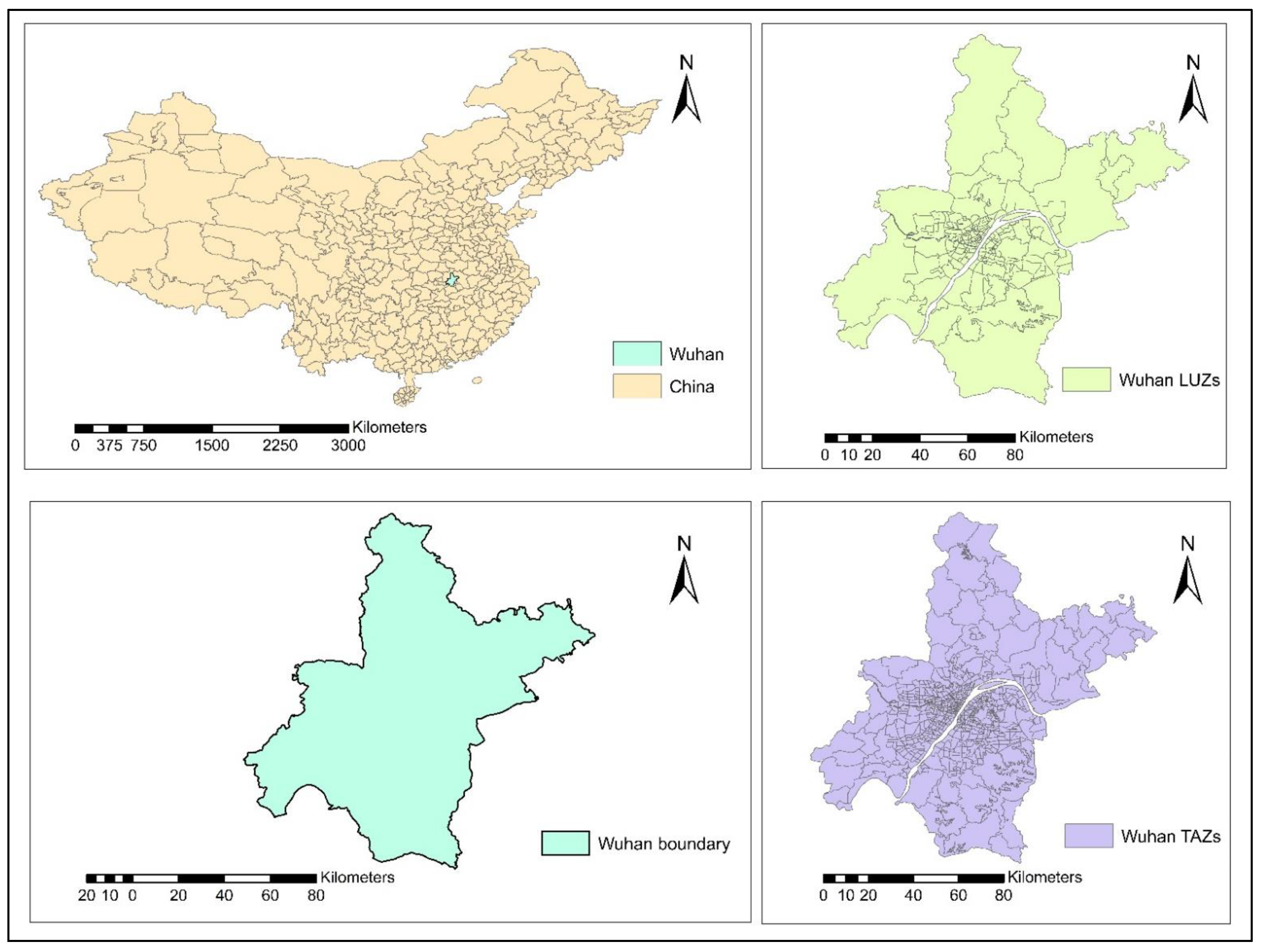
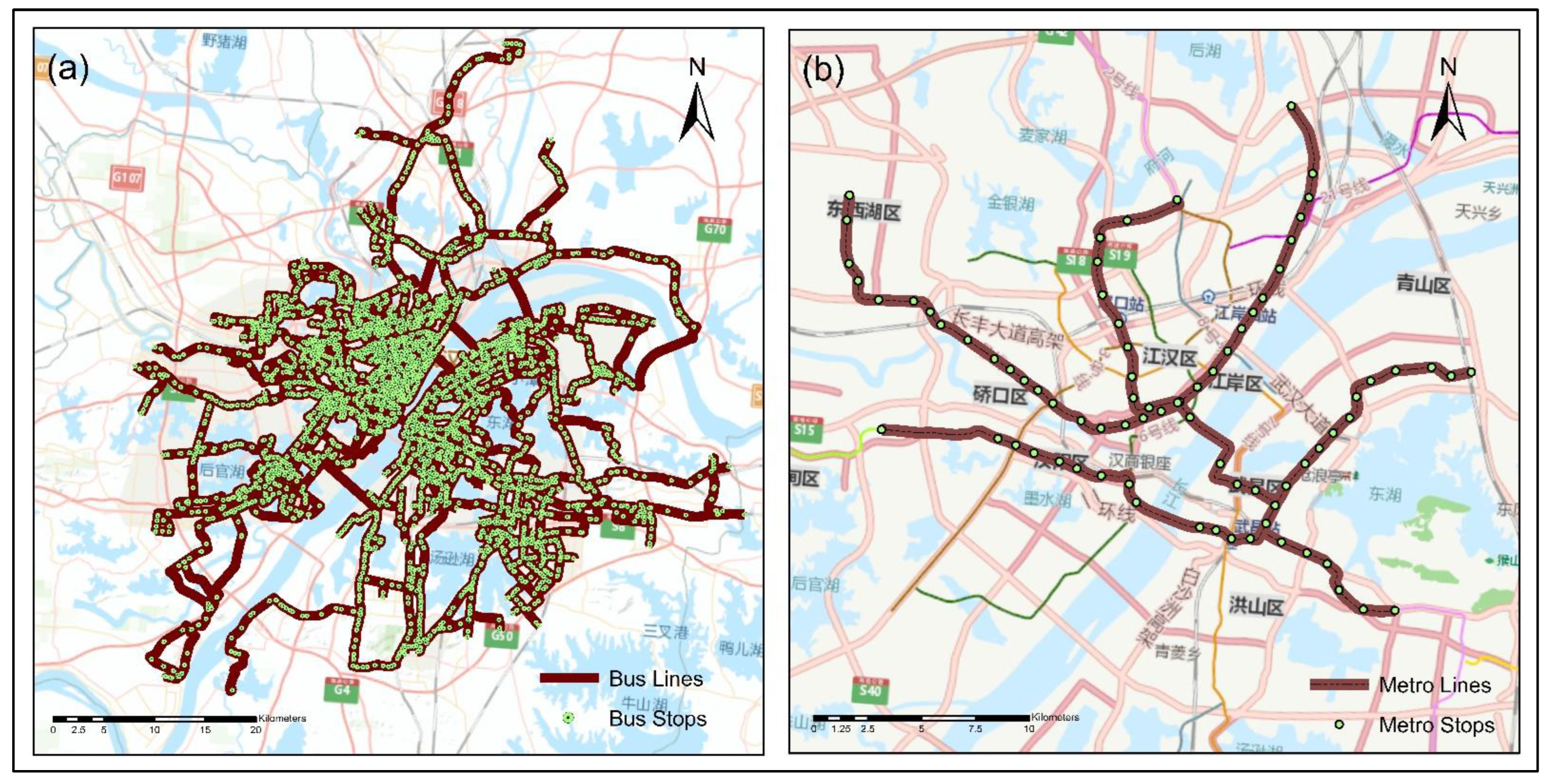
The rest of the paper is sequenced as follows: Section 2 presents an overview of the recent literature regarding accessibility measures and modeling approaches. Section 3 provides the study area and study data including transportation network data and land use data. Section 4 elucidates the methods including the multimodal travel demand model and multimodal integrated spatial economic models. Section 5 explains the study results and discussion. Finally, Section 6 delineates the main findings, limitations, and recommendations for future studies.

2. Literature Review

The accessibility concept was firstly introduced by Hansen in 1959 [24], and he stated that accessibility is the potential of opportunities for interaction and an assessment of the spatial distribution of activities around a point, adjusted for the ability and desire of individuals or firms to overcome physical separation. Accessibility can be broadly defined as the ease with which one place of activity can be accessible from another using a particular mode of transportation or any available modes (such as walking, bus, rail, bike, car, etc.) [25]. Accessibility is defined by Ben-Akiva and Lerman [26] as “the benefits offered by a transportation/land-use system.” Bhat et al. [27] described accessibility as “the ease with which an individual can pursue an activity of a desired type, at a desired place, using a desired mode, and at a desired time.” Accessibility is a primary focus of interdisciplinary research including transportation, health, economics, social sciences, urban studies, and geography [4,28]. The origins of spatial systems can be traced back to Tobler’s law of geography, which states that “everything is connected to everything else, but nearby objects are more connected than distant things” [29]. Primarily, distance, speed, and travel time estimations, also known as impedance measurements, are used to determine accessibility in geographical systems [4]. Evaluating accessibility as the total travel time reduced by road users and the number of additional locations reached by various road users within their budgeted travel time is another practice [30]. In transportation planning, the terms accessibility and mobility are usually confused. Accessibility is the ease of reaching opportunities (goods, services, activities, and destinations), as opposed to mobility, which is the ease of moving people and goods. Mobility falls under accessibility. Accessibility reflects both mobility (the ability of individuals to travel) and land use patterns (the location of activities). This approach provides more importance to nonmotorized modes and accessible land use patterns. Multimodal transportation and more compact, mixed-use, walkable communities tend to optimize accessibility, hence reducing the amount of travel required to reach destinations [31].

In Europe and the United States, we have witnessed a revitalization of city centers over the past two decades, despite the increasing accessibility of metropolitan regions [32]. This re-urbanization is perhaps driven primarily by younger generations, the so-called millennials (roughly, those born in the 1980s and 1990s) [33]. Young households prefer to reside in urban areas that are easily accessible and have enough public transportation, as opposed to the sprawling, automobile-dependent suburbs [33,34]. A previous study on household location preferences in Paris revealed that renters place greater value on a location’s accessibility than owners [35]. Another study conducted in Canada indicated that households were more sensitive to accessibility with time [36]. In addition, Inoa et al. [35] identified commuting time as a crucial element in household decision making, which is true in European cities with larger population densities and better access to public transportation than in developing countries. In developing countries with a high rate of unemployment, households are often ready to travel further or even walk the entire distance to work. Zhang et al. [37] examined public transit-based accessibility to healthcare services in Shanghai. They selected census tracts in central Shanghai that are less accessible to health facilities via public transportation. In contrast, the accessibility of peripheral areas is adequate, despite the lack of neighboring healthcare facilities.

According to a recent study, Ahuja and Tiwari [4] stated that the selection of accessibility measures depends on the context of the application. The fundamental strategy for measuring accessibility can be divided into six categories: (i) Infrastructure approach: this focuses on the speed, travel time, length of the road, density of the road network, and overall congestion level in terms of lost vehicle hours are the major measures. (ii) Activity approach: this focuses on catering to accessing activities. The majority of measures consist of land use and location, potential paths, dwelling, working, recreation, shopping, and the number of activities available within a specific range of travel time or distance. (iii) Individual’s personal preferences approach: this focuses on an individual’s traits, activities, and preferences. Measures range from a person’s socioeconomic variables (car ownership, education, age, and gender) to his or her attitudes and views towards use. (iv) Social exclusion and geographic location approach: this considers an area access/geographical location when the aggregation is at the community level. Although the individualistic method may appear disaggregated and unachievable for inclusive planning, it enables us to understand the fundamental components of all accessibility research. (v) Utility-based approach: this is based on the benefits acquired by people when accessing spatially dispersed activities, opportunities, and challenges, taking into account individual characteristics, characteristics of different transport modes, time budgets, speed, spatial-temporal constraints, and daily activity schedules. (vi) Mixed-measures approach: this is used when there are numerous focal points such as travel costs (monetary, time, risk, comfort, and quality attributes), volume (number of individuals, vehicle units, bus stops, etc.), and location (from one place to another or many places to many places).

The measurements of spatial accessibility are derived from the interaction of three input variables: supply (i.e., locations of infrastructure), demand (i.e., locations of expected infrastructure users), and mobility (i.e., travel costs from demand locations to supply locations). Sometimes, other variables, such as distance decay functions and threshold travel time, are introduced into measurements to indicate the population’s desire to visit infrastructure [38]. In the literature different approach has been employed for the measurement of spatially accessibility such as the gravity model, Shen’s model, and 2SFCA [13]. Firstly, in the gravity model, also known as the cumulative opportunity model, the number of opportunities (i.e., supply facilities) accessible from a given place while taking spatial impedance into account is determined [24]. Secondly, Shen enhanced the precision of geographic accessibility measurement by including a new variable (i.e., demand), whereas the gravity model assumes a homogeneous distribution of individuals [39]. Thirdly, the 2SFCA technique addresses the limitation of Shen’s model, in which every supply facility is assumed to serve every demand location in the case of an inappropriate distance decay function. A threshold travel time is incorporated into the model to reflect the desires of the consumer and to identify the areas accessible within the threshold travel time, such as a catchment area [40].

Several Land Use Transportation Interaction (LUTI) models have been developed over the past decades for location preference and interactions of urban activities, including the Lowry model, IMREL, MEPLAN, TRESSIS, METROSIM, MUSSA, URBANSIM, REURBAN, TLUMIP, TRANUS, DELTA, and PECAS [41,42,43,44,45,46,47,48,49,50,51]. These models estimate production and consumption positions in the metropolitan area using a multi-industry, multi-regional input–output system, with households of various types regarded as labor-producing industries and commodity-consuming industries. PECAS is one of the recently developed integrated land use—transport modeling frameworks. It integrates land use, transportation, the economy, and the environment. The PECAS approach has been implemented in various locations around the world over the last 18 years, including the following: Oregon (statewide), California (statewide), Atlanta, San Diego, Los Angeles, and San Francisco, USA; the City of Edmonton, Province of Alberta, Canada; Caracas, Venezuela; Mumbai, India [52].

In conclusion, each accessibility measure has benefits and drawbacks. Thus, researchers should select the best approach based on their study interests, objectives, and data collection. Most previous research employed a static travel time, such as the peak hour and off-peak hour travel time, to quantify accessibility, assuming that the travel time is fixed and static. These “static” models assume that household locations are static and that transportation supply and opportunities for social practice activities are fixed in time and space, which can lead to biased or even misleading assumptions in accessibility models. Nevertheless, the primary components of accessibility, such as opportunities and social activities, are dynamic and influence the location selection behavior of activities [9]. The majority of previous research evaluated accessibility using a single mode or transit mode with a fixed time, such as peak hours [9,53]. On the other hand, people’s preferences vary according to the time of day and transportation modes. When directly comparing accessibility indicators in different geographical regions, the majority of them fail to account for spatial variability. Hence, it is feasible that high accessibility zones, however, lack public transportation services, which earlier methods cannot identify. Therefore, comparing the degree of public transportation services in areas with similar spatial proximity to urban activity is more reasonable. In this context, by including spatial heterogeneity in the evaluation criterion, this study intends to improve spatial accessibility to urban activities. Furthermore, there has been little research on the accessibility of urban activities such as residential, commercial, and industrial locations. Existing models failed to capture fine features of accessibility, particularly their temporal and mode distribution. The current trends in transportation and urban planning are not sustainable, and improvements in transportation and land use systems are required to meet the needs [54]. Thus, the purpose of this study is to contribute to the current literature by investigating the location choice behavior of urban activities with the MDA employing advanced ISE models, i.e., the PECAS model. The advantages of this method are that it captures very fine details of how various urban activities (such as households, businesses, firms, and so on) are located. The PECAS model is a scientifically sound integrated spatial economic model that has been widely utilized for forecasting and policy formulation at the municipal and regional levels [52].

3. Data Collection

3.1. Study Area

This study considers the City of Wuhan as a Case study, as shown in Figure 1. Wuhan is the capital city of Hubei Province, China. The City of Wuhan is located at 29°58′–31°22′ north latitude and 113°41′–115°05′ east longitude. The City of Wuhan has jurisdiction over thirteen districts. The City of Wuhan includes 690 Traffic Analysis Zones (TAZs) and 147 Land Use Zones (LUZs), with a population of 10.1 million permanent residents by 2012, comprising 6.83 million urban population and 3.28 million rural population. The population increased to 10.6 million by 2015, with the urban population increasing to 7.48 million and the rural population decreasing to 3.11 million because of the urbanization process. As of 2020, the population of Wuhan was 12.48 million (http://tjj.wuhan.gov.cn/tjfw/tjnj/ (accessed on 15 January 2021)).

3.2. Study Data

Urban and rural households and employment by industry type are major datasets used in the development of the M-TDM and ISE models. The rural and urban households and average household size data were obtained from Wuhan statistical Yearbooks (http://tjj.wuhan.gov.cn/tjfw/tjnj/ (accessed on 10 March 2021)). However, the employment by industry data was obtained from Wuhan Transportation Planning Institute (WHTPI). The household travel survey (HTS) data which is a primary source of information that contains all vital information to understand and quantify travelers’ traveling behavior using the actual transport network are obtained from WHTPI (http://www.whtpi.com/Default.html (accessed on 10 March 2021)). This dataset contains, the number of trips by modes, total trip time, trip distance, trip origin and destination, gender, and age of trip makers.

The development of M-TDM for two cross-sectional years, 2012 and 2015, need various levels of networks such as road network and public transit network. The road network contains link type information, link distance, free-flow speed, daily link capacity by link type, and the number of lanes in each road link, as presented in

Table 1. Road network attributes.

Road Network	Description
Link Type	Freeway, expressway, arterial, collector, and local roads
Distance	Link distance (km)
Road Capacity	Daily capacity of each link
Lanes	Number of lanes in each link
AADTs	Average annual daily traffic counts collected at main road corridors
Screen Lines	Screen line number associated with each AADT (used for model calibration)
Speed	Free flow and Congested speed

, and the transit network contains detailed information about transit, as shown in

Table 2. Transit network attributes.

Name	Bus Name/Metro Name
Time	Congested time (minutes)
Distance	Lines distance (km)
Line ID	Bus and Metro line number
Fare	Static fare for bus and distance-based for Metro
Waiting time	Initial waiting time at and transfer waiting time at bus and metro station
Modes	Metro	Bus
Transfer distance allowed (meters)	550 (Metro to bus, metro to metro)	550 (bus to metro, bus to bus)
Walking distance allowed (meters)	960	650
Average Service Frequency of modes (minutes)	5	6

. A well-connected transit network encourages the commuter to use a transit system that enables easy transfer between different transit modes (such as bus to bus, bus to metro, metro to bus, and metro to metro). An extensive transit network was developed to capture the fine details of the transit system. This includes a complete representation of transit lines and stations, transfer times, transfer links, walking to and from transit stations, different transit fare systems (static fare system for bus and distance-based fare system for metro), and other relevant information presented in Table 2. Figure 2 depicts the transit network of Wuhan, China, in 2015, including the metro, bus, and their corresponding stations.

Walking and transfer distance thresholds are specified to enable transfer with the specified distance limits. The transfer distance thresholds are used to avoid the generation of unnecessary non-transit legs during the route enumeration process. Two curves were developed to calculate waiting and transfer times, as shown in Figure 3.

The initial waiting time curves were used to calculate the initial perceived waiting time (minutes) at bus and metro stations. The initial waiting time calculated is half of the headway, as shown in Figure 3. Meanwhile, the transfer waiting time curve is developed to calculate transfer waiting time at bus and metro stations. Usually, the transfer waiting time is perceived differently compared to the initial waiting time as shown in Figure 3. Most of the commuters prefer direct routes which involve no transfer or minimal transfer waiting and walking times. The initial waiting time and transfer waiting time were used during the route evaluation process to find the best path from origin ‘i’ to destination ‘j’, with minimal walking, transfer, and travel cost.

Land Use Data

The land use data in Figure 4 shows aggregate spatial input–output data which represents the interaction of activities and commodity flows. These input values represent the amount of economic activity for a particular combination of sectors. The land use data includes various industrial sectors (such as agriculture, industry, and commercial household activities (such as urban and rural), commodity types (including agricultural products, industrial products, commercial products, and transport products), labor types (such as management and technical labor, retail labor and outdoor labor) and space types (such as residential, commercial and industrial). For instance, household activity produced labor and consumed various commodities during this process, and it also consumed residential space during the allocation process, which could be done at either LUZ or TAZ level.

4. Method

In this study, a M-TDM was developed at the TAZ level to calculate MDA to various activity locations (such as households and commercial). Additionally, the accessibility measures from a multimodal are input into ISE models such as the PECAS model. The ISE model estimates the locations based on MDA measures inputs, and as a result, it influences the location/allocation of urban activities (such as households, businesses, firms, etc.) over time and space [47]. This study used an advanced transport modeling tool, Cube Voyager version 6.5, and ArcGIS version 10.8 software to develop a multimodal transport system.

4.1. Multimodal Travel Demand Model

The developed M-TDM is used to calculate MDA (such as time, distance, and logsum) to various activities located within the study area. The M-TDM for the years 2012 and 2015 is developed using socioeconomic data (such as population, and employment). Additionally, M-TDM is calibrated and validated for the years 2012 and 2015. The developed M-TDM model for the years 2012 and 2015 was used to calculate MDA for goods, services, labor, and other activities, as shown in Figure 5.

As discussed earlier, a multimodal transport model was developed for the years 2012 and 2015 using the road network, transit routes, LUZs, and TAZs. The M-TDM development starts with the calculation of trip production and attraction rates using population, employment, and household travel survey data. The friction factors (FF), which are input into trip distribution, were calculated using the travel survey data. Furthermore, the FF are smoothed using the gamma distribution approach before being input into the trip distribution model. Trip length frequencies by trip purpose were calibrated and verified against the observed trip lengths obtained from travel survey data. Transport utilities by trip purpose (such as home-based work, home-based other, home-based school, and non-home-based) and by modes (such as metro, bus, taxi, personal car, and bike) were calculated and input into the nested logit model, as shown in

Table 3. Transport utilities by modes.

	Home-Based Work (HBW) Car Available						Home-Based Other (HBO) Car Available
Modes	α1	α2	α3	α4	α5	α6	α1	α2	α3	α4	α5	α6
Metro	−0.02	−0.04	−0.04	−0.039	−0.1	−0.2	−0.02	−0.04	−0.04	−0.078	−0.1	−0.2
Bus	−0.02	−0.04	−0.04	−0.039	−0.2		−0.02	−0.04	−0.04	−0.078	−0.2
Taxi	−0.02	−0.04	−0.039				−0.02	−0.04	−0.078
Car	−0.02	−0.04	−0.039				−0.02	−0.04	−0.078
Bike	−0.02	−0.04					−0.02	−0.04
	Home-based school (HBS)						Non-home-based (NHB)
Modes	α1	α2	α3	α4	α5	α6	α1	α2	α3	α4	α5	α6
Metro	−0.02	−0.04	−0.04	−0.305	−0.1	−0.2	−0.02	−0.04	−0.04	−0.114	−0.1	−0.2
Bus	−0.02	−0.04	−0.04	−0.305	−0.2		−0.02	−0.04	−0.04	−0.114	−0.2
Taxi	−0.02	−0.04	−0.305				−0.02	−0.04	−0.114
Car	−0.02	−0.04	−0.305				−0.02	−0.04	−0.114
Bike	−0.02	−0.04					−0.02	−0.04

. The value of α varies depending on trip purpose and availability of a personal car. In this study, home-based work and home-based other trips by car are considered. As mentioned in Section 3.2, the various modes of transportation attribute coefficients such as in-vehicle time, waiting time, walking time, metro and bus fare, transfer time, and cost per km by different trip purpose (HBW, HBO, HBS, and NHB) were obtained from the Wuhan Transportation Planning Institute (WHTPI) (http://www.whtpi.com/Default.html (accessed on 10 March 2021)).

Equations (1)–(5) determine the individual’s preferences for a specific transport mode for specific trip purposes. The structure of the nested logit model is illustrated in Figure 6.

U_Metro = α1 × IVT + α2 × IWT + α3 × WT+ α4 × MF + α5 × MMTT+ α5 × MTBT

(1)

U_Bus = α1 × IVT + α2 × IWT + α3 × WT + α4 × BF + α5 × TT

(2)

$${\mathrm{U}}_{\mathrm{Taxi} }= \mathsf{\alpha }1\times \mathrm{IVT} + \mathsf{\alpha }2\times \mathrm{WT} + \mathsf{\alpha }3\times \mathrm{DC}$$

(3)

U_Car = α1 × IVT + α2 × WT + α3 × DC

(4)

U_Bike = α1× IVT + α2 × WT

(5)

where the following are defined:

–

IVT = in-vehicle time (actual time);

–

IWT = initial waiting time at bus and metro station;

–

WT = walking time from home to bus and metro station;

–

MF = metro fare;

–

MMTT = metro-to-metro transfer time;

–

MTBT = metro-to-bus transfer time;

–

BF = bus fare;

–

TT = bus-to-bus and bus-to-metro transfer time;

–

WT = waiting time (in case of taxi), access time in case of car and bike;

–

DC = cost per km drive.

The mode choice module uses congested travel time, transport utilities, and scaling parameters (calculated and calibrated against observed mode shares by mode type) to split trips by different modes. Finally, network assignment (user-equilibrium) and transit assigned (multi-routing) is calculated and calibrated against annual average daily traffic (AADTs) counts. The M-TDM calibration was performed at trip generation, distribution, mode choice, and assignment level. After the M-TDM was fully calibrated and converged, the MDA measure was calculated using Equation (6).

$$A_i=\ln {\displaystyle \sum }_{j=1}^n{e}^{\left({\varphi }_{T}Transpor{t}_{UMij}\right)\times O_J}$$

(6)

where the following are defined:

–

$A_i$ = Utility-based accessibility measure;

–

${\mathrm{Transport}}_{UMij}$ = Transport utility (disutility) from origin i to destination j using mode M;

–

${\varphi }_T$ = Transport Coefficients (these represent the sensitivity of commuters to mode and trip type;

–

$O_J$ = Opportunities at destination zone j (in the case of households, jobs are considered as the opportunities, while in the case of commercial services, the residential population is considered as the opportunity).

Furthermore, the MDA (congested mode-specific skims), which is input into the ISE model, is used to calculate the locational preferences of urban activities as shown in Figure 5.

4.2. Multimodal Integrated Spatial Economic (ISE) Models

Several ISE models (such as auto-based, metro-based, bus-based, and transit-based) were used in this study. The graphical representation of the ISE model framework is depicted in Figure 7. The major components of the developed ISE models are:

• Economic and demographic module: This module consists of economic and demographic information about the study area including population and employment.
• Activity Allocation (AA) module: The AA module of the multimodal ISE model is using nested and additive logit theory, for the location/allocation of urban activities. The AA module of the ISE model is an aggregate representation of urban activities, commodities flow between origin and destination, markets (selling and buying) with aggregate demands and supplies, and exchange prices, which are usually determined at the exchange locations.
• Space development (SD) module: The SD module of the multimodal ISE represents real-estate developer behavior (developed space based on the market demand). This module is sensitive to market prices and developed space accordingly.
• Transport module: The transport model was developed to calculate MDA for various activity locations within the study area, for the years 2012 and 2015.

As mentioned earlier SD module uses the price signal (market prices sets during location/allocation of activities) to develop the space. The formulation of the SD module is given in Equation (7).

$$F=max\left[ 1, F_b+\exp \left(\frac{\left(P\ast \beta -P_b\right)}{P_b}\right)\right]$$

(7)

where the following are defined:

–

$F$ = Factors applied to the current space;

–

$\beta$ = Scale factors;

–

$P$ = Current price;

–

$P_b$ = Base price.

The factors represent the growth factors applied to the current floor space, which is further input into the next modeling yea (Year T+1).

The primary function of the M-TDM is to provide access to other people and companies so that they can participate actively in all kinds of spatially and temporally distributed activities (social, economic, etc.) and exchange information, goods, and services in a physical manner [18]. The AA module represents activity locations that occur as a result of the location choice behavior of activities based on the nested and additive logit approaches.

The locations considered for this study were TAZs which were large enough to be distinct markets for the location/allocation of various activities over time and space. The relation between MDA and location choice of activities is well understood using mode-specific ISE models. To evaluate the locational choice behavior of activities using MDA, it is important to understand which mode influences the locational preferences of activities more. The specific modes used in the study considered the auto mode (car and taxi), metro, bus, and combination of bus and metro (transit) for both production and consumption of urban activities.

4.3. Simulating Activity Location Choices with the ISE Model

The random utility maximization approach was adopted to simulate the location decisions of the activities (household and industrial sector). It is assumed that the agents (such as households, businesses, and firms) assign a utility to each zone and choose the one that maximizes it. In the ISE, joint choice utility is calculated using Equation (8).

$$Utilit{y}_{d,k}=\frac{1}{\lambda }ln{\displaystyle \sum }_{z=0}^n{e}^{\lambda \left({\varphi }_{T,d}Transpor{t}_{z,k,d,M}+{\varphi }_{p,d}Pric{e}_{z,d}+\frac{1}{\lambda }lnSiz{e}_{z,d}\right)}$$

(8)

–

D = buying (consuming) or selling (producing) the commodity;

–

k = index for zone of production or consumption of the commodity;

–

z = index for an exchange zone;

–

$\lambda$ = dispersion parameter for the exchange location choice for the commodity;

–

${\mathit{Size}}_{z,d}$ = an indicator of the relative amount of the commodity offered in exchange zone z;

–

${\varphi }_{T,d}$ = transport cost coefficient;

–

$Transpor{t}_{z,k,d,T}$ = transport cost between z and k for d = buying and selling, M = transporting modes;

–

${\varphi }_{p,d}$ = price coefficient (always set to 1 for d = selling and −1 for d = buying because the utility is in monetary units);

–

Price z = price of a commodity in z;

–

Ln = natural log.

The utility of transporting a unit of each commodity from origin to destination zone was using the transport attributes from M-TDM.

5. Results and Discussion

5.1. Results

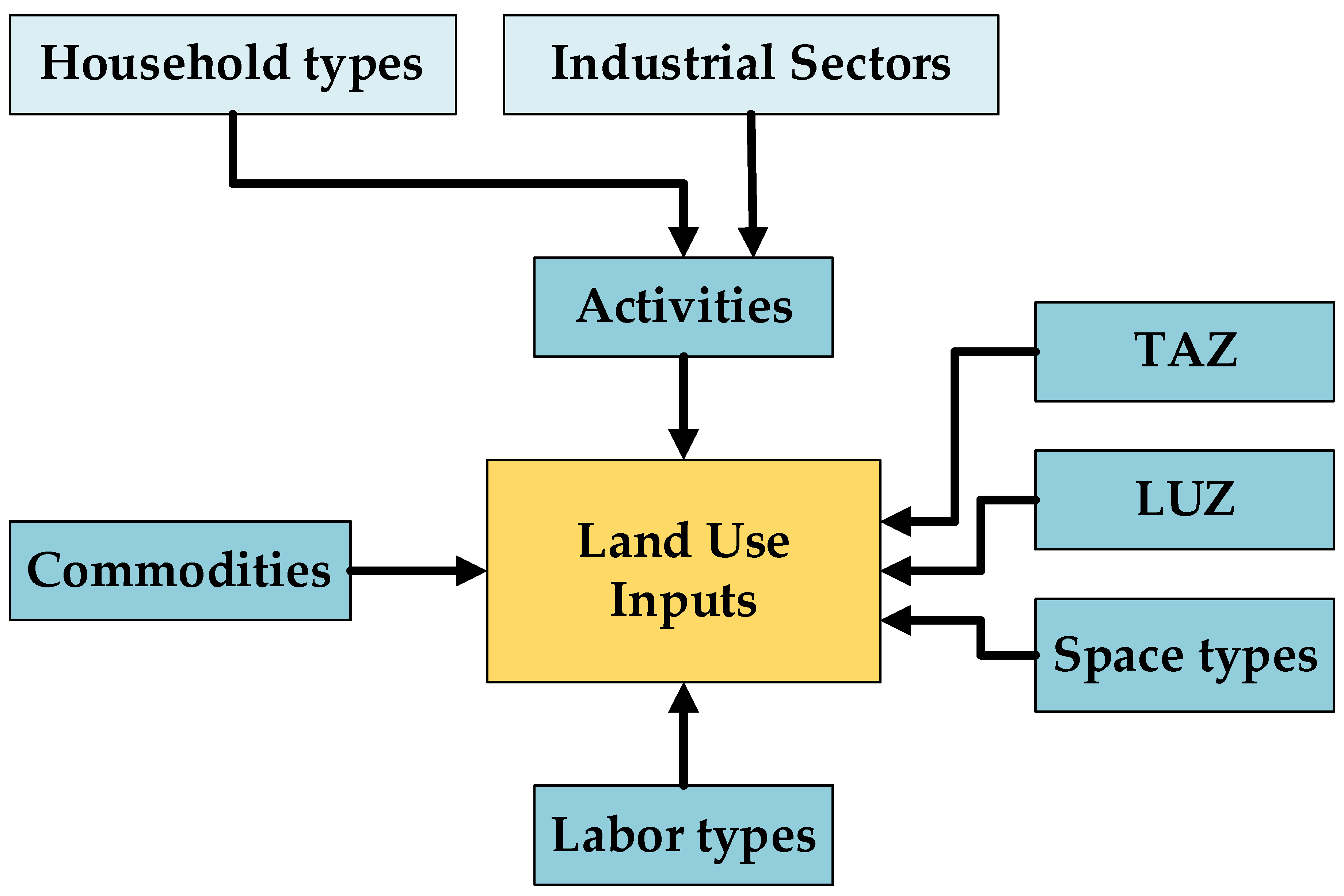
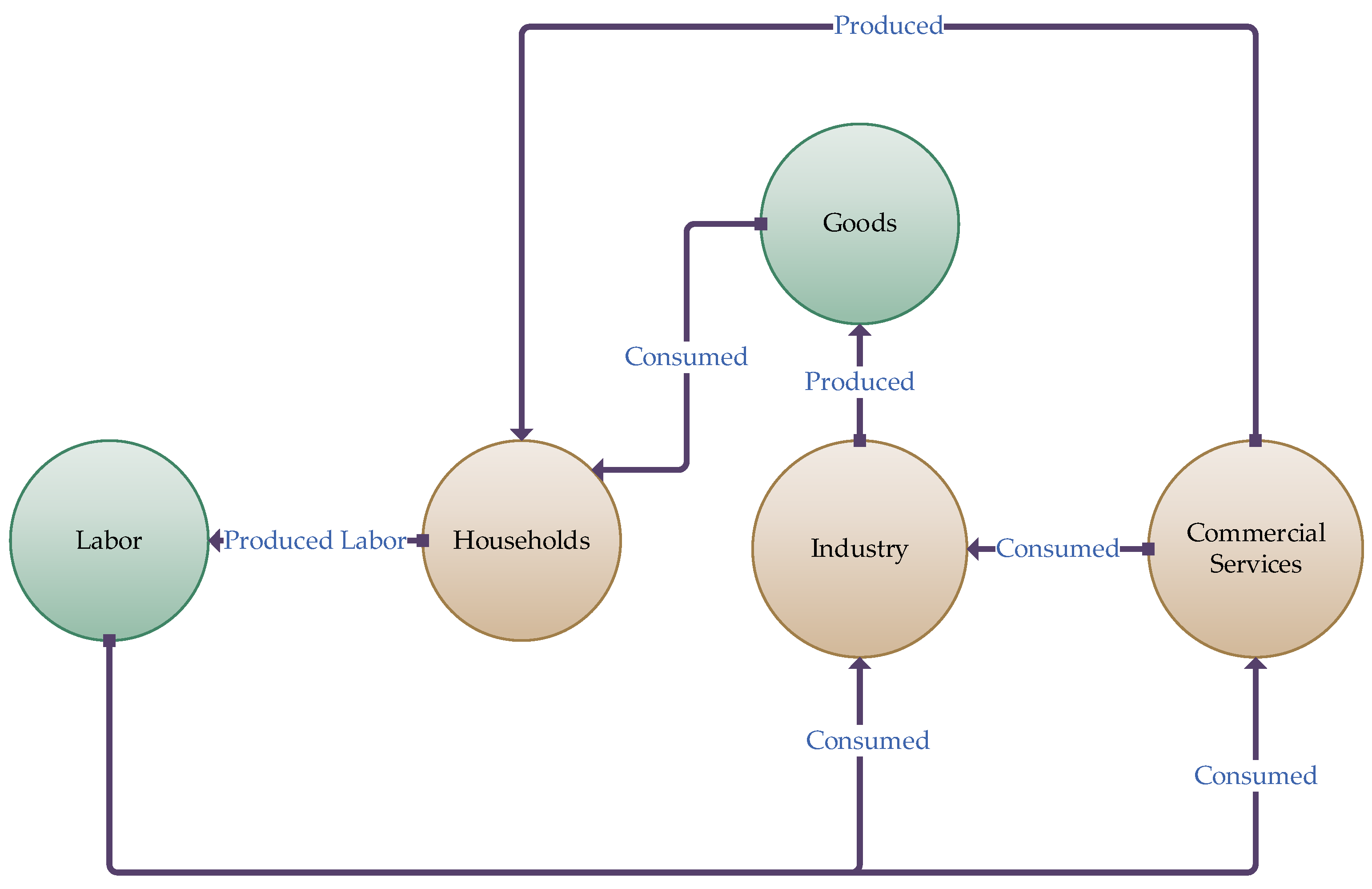
The developed multimodal ISE models were used to determine the relationship between MDA and location preferences of urban activities within the study area. In the case of ISE models, the households are producers of labor, and this labor is consumed by industries and firms during the production process. Likewise, firms and industries are the producers of jobs, and these jobs are consumed by households. The location choice behavior of household and industrial sector activities was further classified: (i) locational preferences of household activities; (ii) locational preferences of commercial services (household-obtained services such as retail services).

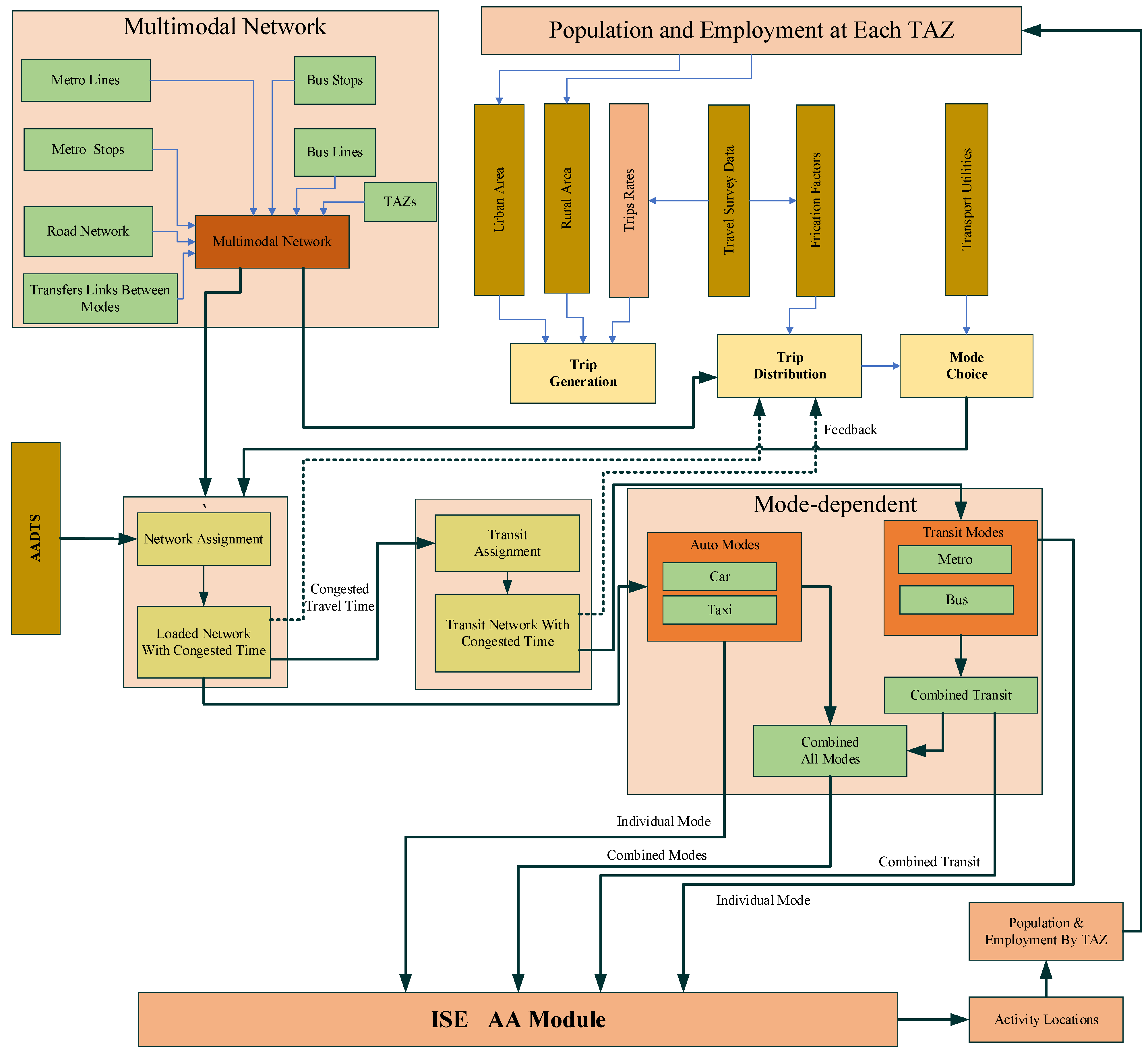
In general, most economic activities rely on an appropriate level of accessibility to survive and progress; hence, a variety of accessibility approaches must be considered. As previously stated, for the years 2012 and 2015, M-TDM was built, calibrated, and validated before being used to calculate MDA. The MDA measure is used to calculate short-term dynamic accessibility to goods, services, and other activities located in the City of Wuhan using different modes. The MDA considers only main modes of transport (such as auto, bus, and metro) and excludes non-motorized modes such as walking and biking as they do not affect traffic congestion. The flow of commodities from where they are produced to where they are consumed influence the transport system. The location/allocation of these activities changes the attractiveness of the location for households, businesses, and firms. The utilities (Equation (8)) are critical in driving decisions in the ISE system. These utilities influence the location choice behavior of households, businesses, and industries. Because these activities are subject to commodity utilities, changes in the utility function affect consumers and producers of the given commodity for households and other activities.

Goods and services are grouped based on their defined industry. These groups interact with each other over time and space using a transport system. Households are social units that typically provide labor, and consume goods and services. Meanwhile, as illustrated in Figure 8, industries, firms, and businesses produce goods and consume labor during the location/allocation process.

Table 4. Locational preferences of activities parameters.

Activity Type	Commodity	Labor, Services, and Goods Type	Consume By	Transport Modes	Utility (Disutility)
Households	Labor	Management and technical labor	Industry and services	Auto, bus, metro, and combinations	logsum
		Retail service labor
		Operators labor Other labor
Commercial services	Services	Commercial services	Households and industry

depicts activities, commodities, and their production and consumption process. The connectivity between TAZs is based on the congested network (time, distance, logsum, etc.) by different modes. The transport utilities which, in transport terms, are referred to as disutilities are used by the ISE model during the location/allocation process. These disutilities influence the buying and selling of various commodities at each TAZ.

The primary hypothesis is that residents prefer a location close to their job place or prefer a place with high accessibility to their primary needs using a specific transport mode. The results revealed that the actual influence of residential location and accessibility to the desired job location depends primarily on the underlying geographical location (spatial) and temporal (transport mode).

Overall, the R² for the models show a strong relationship between MDA and residential locations where most of the adjusted R² value were found higher than 0.81. Results revealed that there is a significant improvement in the residual square from the year 2012 to 2015, due to the improved level of transit accessibility in the year 2015, as shown in

Table 5. Results for the MDA to household activities.

Year		2012	2015
Auto	Residual Squares	23.79	59.16
	R2	0.71	0.79
	Adjusted R2	0.63	0.75
Bus	Residual Squares	49.72	102.50
	R2	0.46	0.64
	Adjusted R2	0.32	0.62
Metro	Residual Squares	49.98	102.06
	R2	0.46	0.64
	Adjusted R2	0.32	0.63
Transit	Residual Squares	21.34	43.77
	R2	0.77	0.85
	Adjusted R2	0.70	0.81

.

Table 6. Results for the MDA to commercial activities.

Year		2012	2015
Auto	Residual Squares	493.37	142.87
	R2	0.72	0.84
	Adjusted R2	0.69	0.80
Bus	Residual Squares	550.60	137.70
	R2	0.50	0.53
	Adjusted R2	0.49	0.49
Metro	Residual Squares	547.63	136.73
	R2	0.70	0.70
	Adjusted R2	0.63	0.63
Transit	Residual Squares	35.52	2.52
	R2	0.81	0.91
	Adjusted R2	0.81	0.89

presents the results for the MDA to commercial activities. Overall, the results showed that there is a strong relationship between MDA and commercial locations. For the years 2012 and 2015, the adjusted R² value for transit was 0.81 and 0.89, respectively. Additionally, the results indicated that transit accessibility to commercial locations had a high R² value as compared to auto, bus, and metro.

Accessibility indexes (AI) provide a synthetic measurement of the ability to reach a particular type of opportunity from a place of origin using a particular type of mode used to present the MDA levels at each TAZ. For instance, higher values of AI represent high accessibility using specific transport modes. Meanwhile, the household location index (HLI) and commercial location index (CLI) terms are used to represent the ISE model estimated household and commercial locations. For instance, higher values of HLI and CLI represent a high density of household and commercial locations in each TAZ, while low HLI and CLI represent the low density of household and commercial locations in each TAZ.

5.1.1. Locational Preferences for Household Activities

Labor is produced by households and consumed by businesses, firms, and other industries. The industry sectors including import and export, labor wages, production, and consumption are defined in terms of the (Chinese Renminbi—RMB) and households are defined in terms of household numbers. The commuting costs between origin and destination for commodity flows are calculated during the model run, and wages of labor are adjusted to match the supply and demand in each location for each occupation. The occupation in each industry was used to categorize employment by industry.

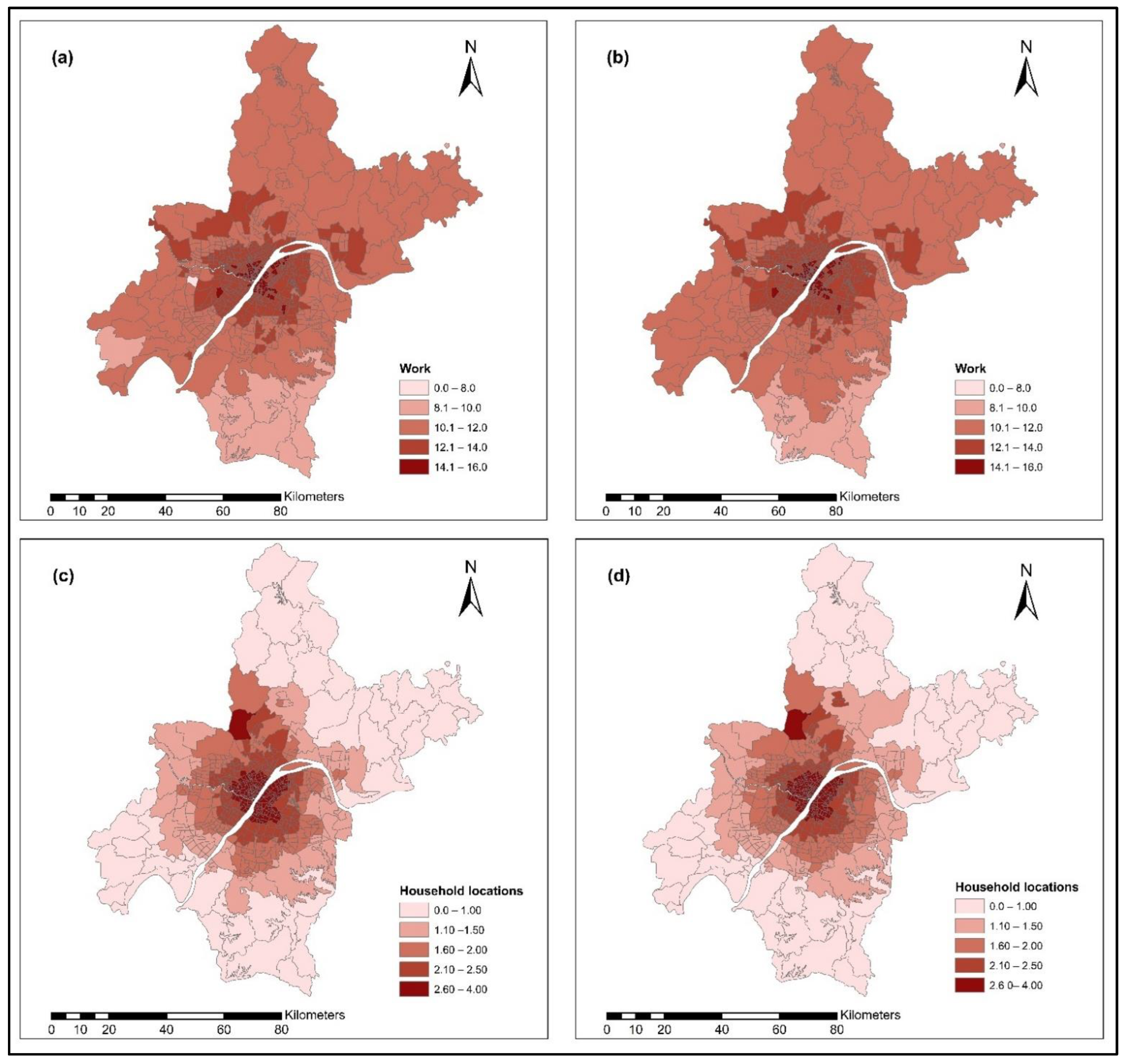
Figure 9a,b shows the result of AI to household activities (such as accessibility to work and other activities) for the years 2012 and 2015 using auto (car and taxi) mode. The results revealed that most of the study area was accessible using auto as a commuting mode. Additionally, it was found that the AI, especially in the downtown areas where most households lives and work, were high (AI ranges between 12–16), as shown in Figure 9a,b. However, this result is intuitive that a majority of households living in the downtown area prefer other modes such as metro and bus for their daily commute. In Figure 9a,b, the ranges of AI values indicate the following: low accessibility (0~8.0); low–medium accessibility (8.1~10); medium accessibility (10.1~12); medium–high accessibility (12.1~14); high accessibility (14.1~16).

As indicated earlier, auto as a commuting mode provides accessibility to the entire study area; as a result, it was found that households with private cars prefer locations with high auto accessibility. The household location index (HLI), which is the result of the allocation process (Equation (8)), is adopted to indicate the location choice behavior of urban activities. Figure 9c,d presents the range of HLI as a result of ISE estimations using auto-based accessibility for the years 2012 and 2015. The HLI ISE-estimated value ranges using auto mode are as follows: low level of household locations (0.0~1.0); low–medium level of household locations (1.1~1.5); medium level of households location (1.6~2.0); medium–high level of household locations (2.1~2.5); high level of household location (2.6~4.0).

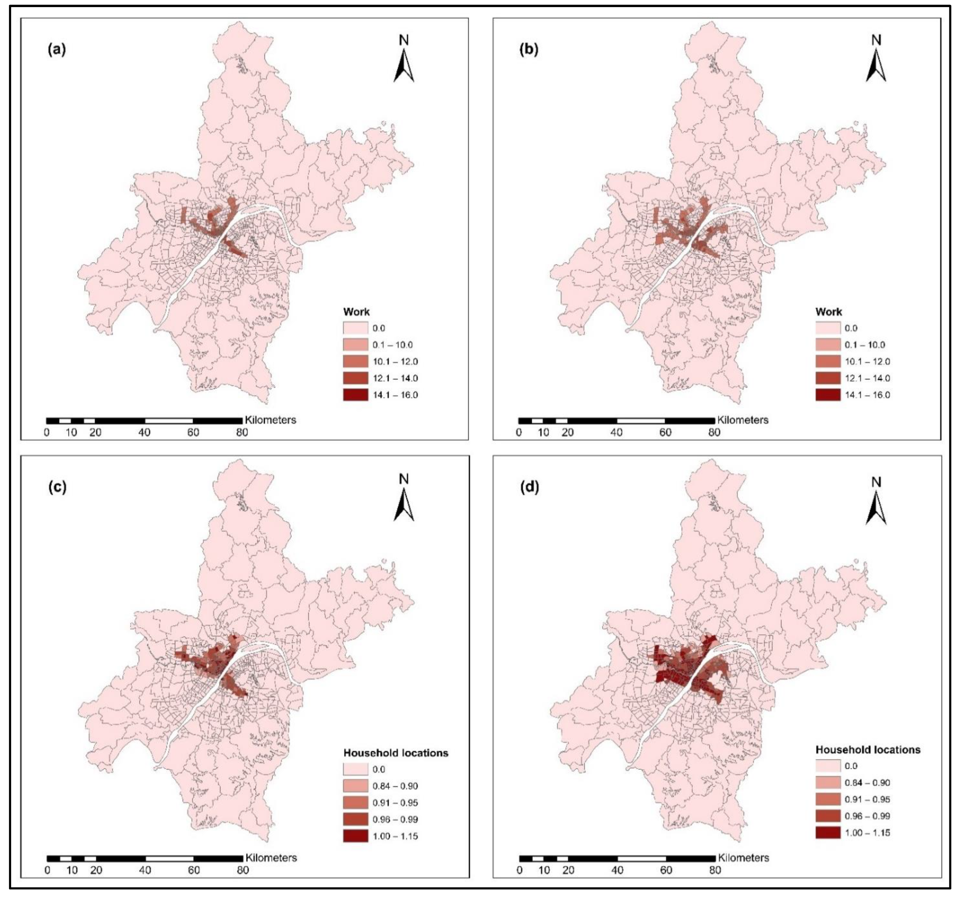
Figure 10a,b shows accessibility to household activities (such as accessibility to work and other activities) using the metro for the years 2012 and 2015. In 2012, there were only two metro lines; however, in 2015, there were three metro lines with limited stations, which only provided access to a limited area. In Figure 10a,b, the range of AI values represents no accessibility (0.0), low–medium accessibility (0.1~10), medium accessibility (10.1~12), medium–high accessibility (12.1~14), and high accessibility (14.1~16).

Figure 10c,d presents the range of HLI as a result of ISE estimations using metro-based accessibility for the years 2012 and 2015. The HLI ISE-estimated value ranges using metro mode are as follows: no household locations (0.0); low–medium level of household locations (0.84~0.90); medium level of households location (0.91~0.95); medium–high level of household locations (0.96~0.99); high level of household location (1.0~1.15).

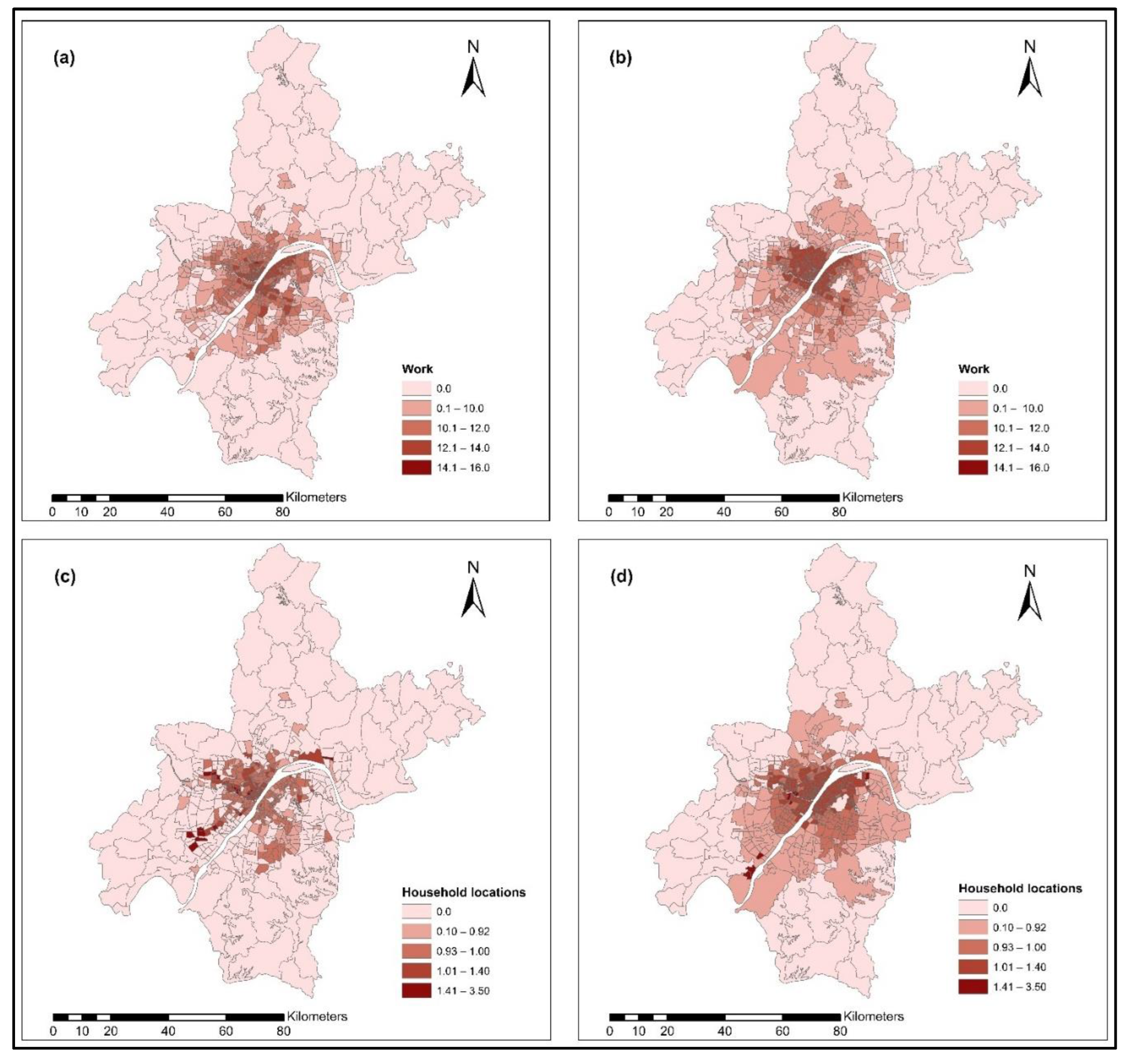
Compared to the metro, bus services covered most of the downtown area during the years 2012 and 2015. The bus provides accessibility to most of the household activities located in the downtown area and its surrounding areas. Figure 11a,b indicates the accessibility to household activities using bus mode for the years 2012 and 2015. The range of AI values represents the following: no accessibility (0.0); low–medium accessibility (0.1~10); medium accessibility (10.1~12); medium–high accessibility (12.1~14); and high accessibility (14.1~16).

Meanwhile, accessibility to household activities using bus mode and the ISE-estimated household locations results indicate that areas with a high level of bus accessibility showed a high level of household location and most of the values were related to household locations. Figure 11c,d presents the range of HLI as a result of ISE estimations using bus-based accessibility for the years 2012 and 2015. The HLI ISE-estimated value ranges using bus mode are as follows: no household locations (0.0); low–medium level of household locations (0.1~0.92); medium level of households location (0.93~1.0); medium–high level of household locations (1.01~1.11); high level of household location (1.12~1.33).

Transit (metro and bus) provide interconnected services which provide transfer between these modes. To make this an attractive commuting mode, a discount fare policy is introduced by the local government to encourage the transfer between bus and metro. Transit accessibility results indicate that accessibility to household activities using transit significantly increased during the year 2015, and most of the AI values are in the range 10–16, especially during the year 2015, due to the updated transit system. Figure 12a,b indicates the accessibility to household activities using transit for the years 2012 and 2015. The range of AI values represents the following: no accessibility (0.0); low–medium accessibility (0.1~10); medium accessibility (10.1~12); medium–high accessibility (12.1~14); high accessibility (14.1~16).

Meanwhile, the ISE-estimated household locations using transit accessibility indicated that areas with a high level of transit accessibility showed high household locations. During 2015, most of the household location values are in the range 1.01–3.5, due to improved transit accessibility. Figure 12c,d indicates the range of HLI as a result of ISE estimations using transit-based accessibility for the years 2012 and 2015. The HLI ISE-estimated value ranges using transit are as follows: no household locations (0.0); low–medium level of household locations (0.1~0.92); medium level of households location (0.93~1.0); medium–high level of household locations (1.01~1.40); high level of household location (1.41~3.50). These results indicate that transit accessibility to household activities has a strong relationship with household locations.

The household locations of the ISE model results showed the same trend, namely, as accessibility increases, household activity locations increase, which is presented in Figure 9a–d and Figure 12a–d.

5.1.2. Locational Preferences of Commercial Activities

Commercial activities or services (such as information, retail, hospitality, real estate, technical services, environmental services, and private services), such as household activities, are vital in any economic system. However, in the ISE system, an aggregate ‘commercial activity’ phrase is employed to represent commercial services.

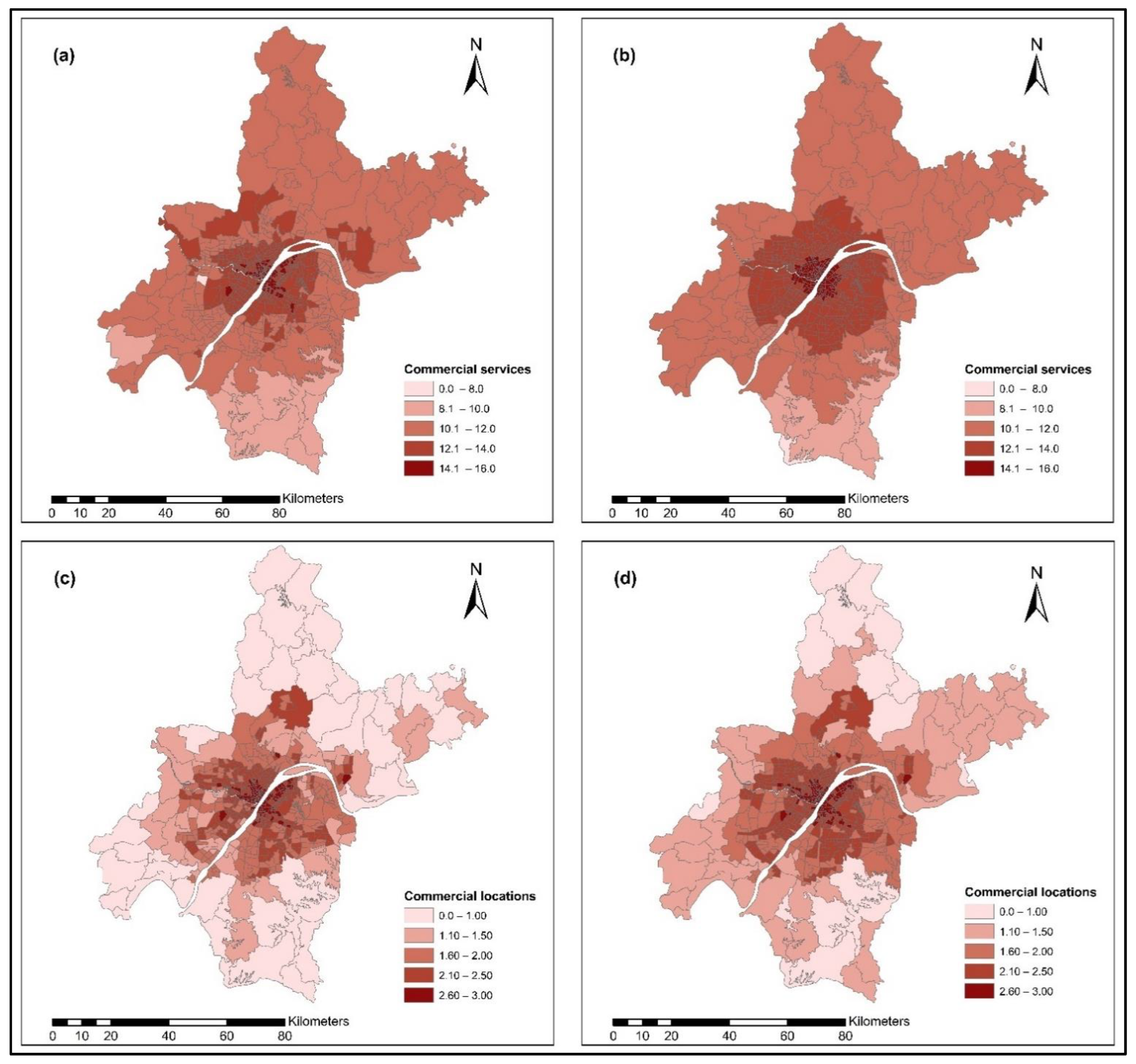
Figure 8 depicts the commercial activity buying and selling procedure process. Commercial activities typically buy labor and sell services to other activities, including households, and in the process consume a variety of other commodities and services. The enhancement of the road network and transit services increases accessibility and the location choice behavior of commercial services, with better accessibility attracting more commercial activity. Commercial activities (services obtained by households) prefer locations with low transport costs. However, it may vary depending on the nature of the commercial activity; some services are sensitive to auto accessibility, while others are sensitive to accessibility via other modes. It was revealed that the level of auto accessibility to household activities in 2015 was considerably high compared to 2012. Figure 13a,b indicates the range of auto accessibility to commercial activities for the years 2012 and 2015. The AI represents the following: low accessibility (0~8); low–medium accessibility (8.1~10); medium accessibility (10.1~12); medium–high accessibility (12.1~14); high accessibility (14.1~16).

Meanwhile, the ISE-estimated commercial locations are presented in Figure 13c,d. The results revealed that areas with high auto accessibility to commercial services showed a high level of commercial locations. Figure 13c,d shows the range of CLI as a result of ISE estimations using auto-based accessibility for the years 2012 and 2015. The CLI ISE-estimated value ranges using auto are as follows: low commercial locations (0.0~1.0); low–medium level of commercial locations (1.1~1.50); medium level of commercial locations (1.60~2.0); medium–high level of commercial locations (2.1~2.50); high level of commercial locations (2.6~3.0).

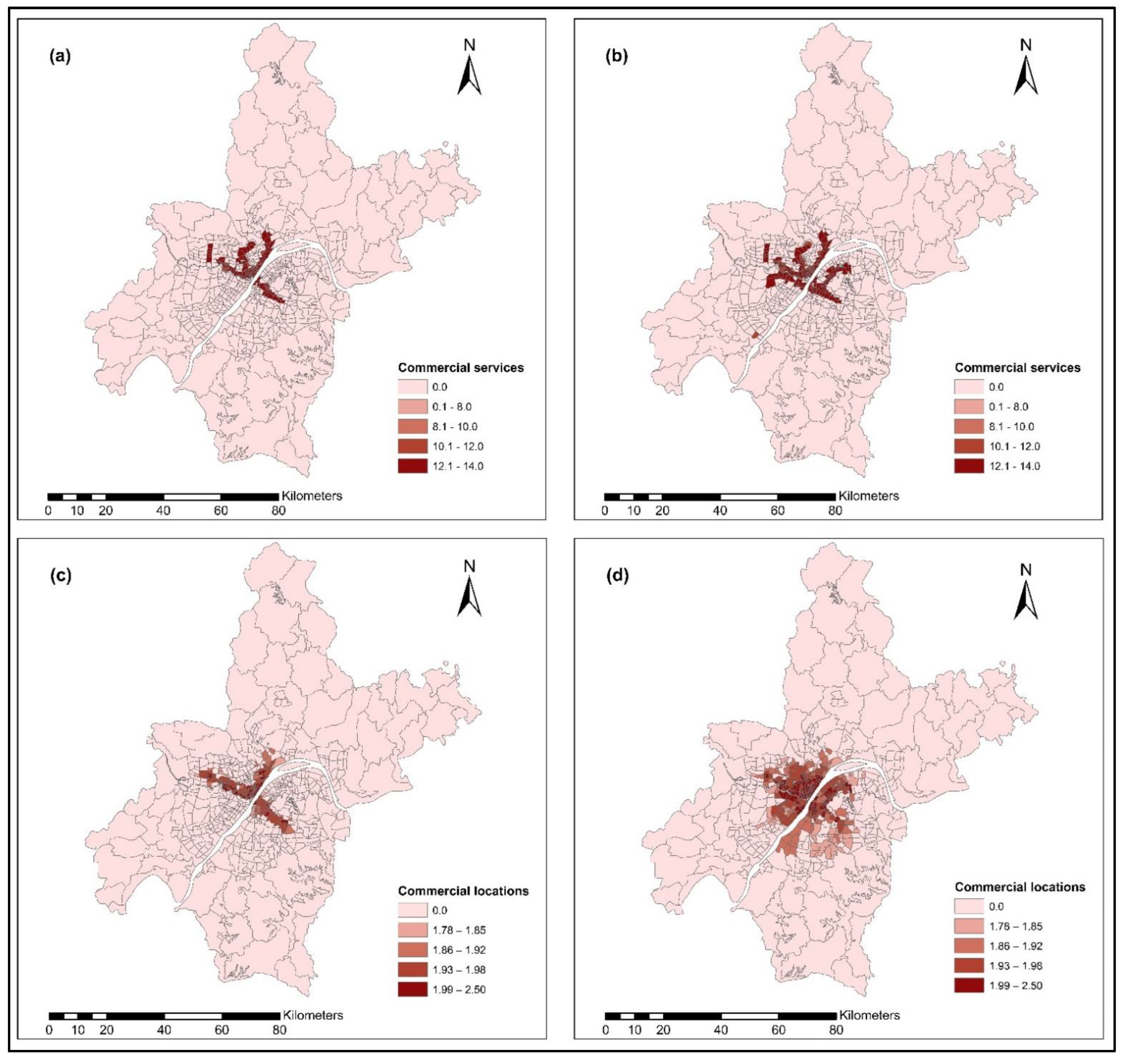
Figure 14a,b presents the result of metro accessibility to commercial services during 2012 and 2015. In 2015, metro accessibility to commercial services was relatively high compared to 2012, because of the new metro line, and most of the AI values are in the range 10–14. Figure 14a,b indicates the range of metro accessibility to commercial activities for the years 2012 and 2015: low accessibility (0.0); low–medium accessibility (0.1~8); medium accessibility (8.1~10); medium–high accessibility (10.1~12); high accessibility (12.1~14).

Meanwhile, Figure 14c,d results also reveal that areas with high metro accessibility to commercial services showed a high level of commercial locations, especially in the year 2015. The CLI ISE-estimated value ranges using metro are as follows: no commercial locations (0.0); low–medium level of commercial locations (1.78~1.85); medium level of commercial location (1.86~1.92); medium–high level of commercial locations (1.93~1.98); high level of commercial location (1.99~2.50).

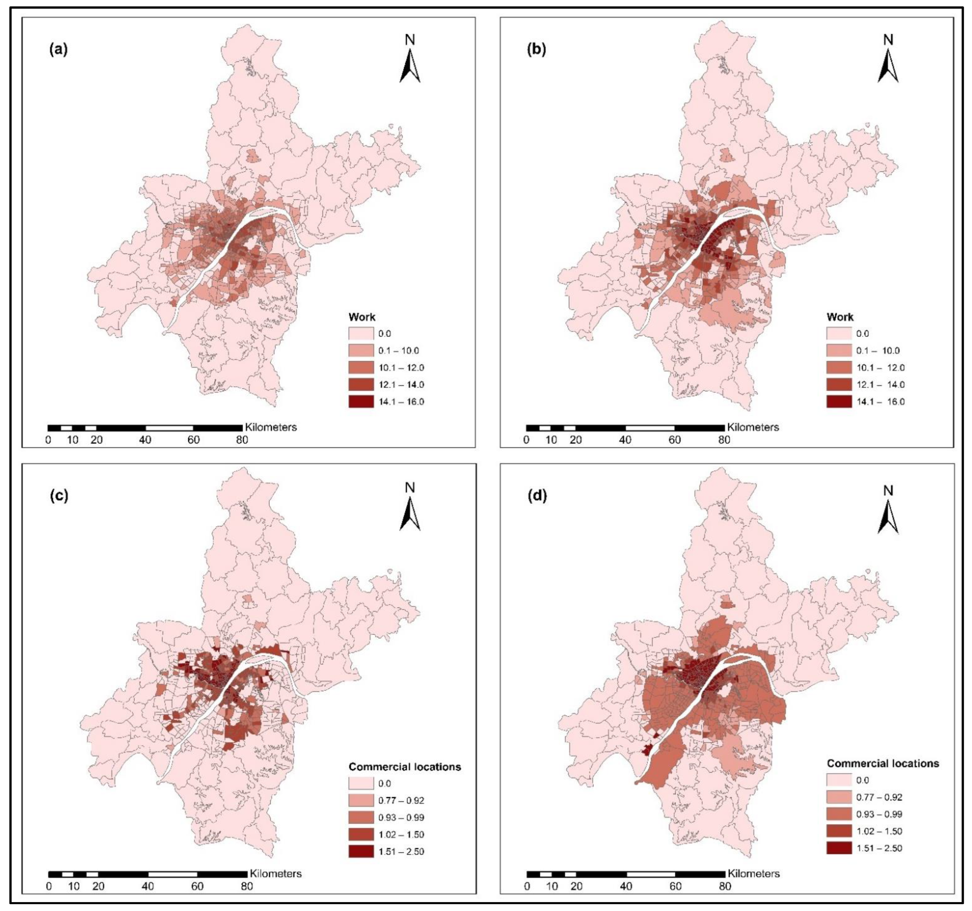
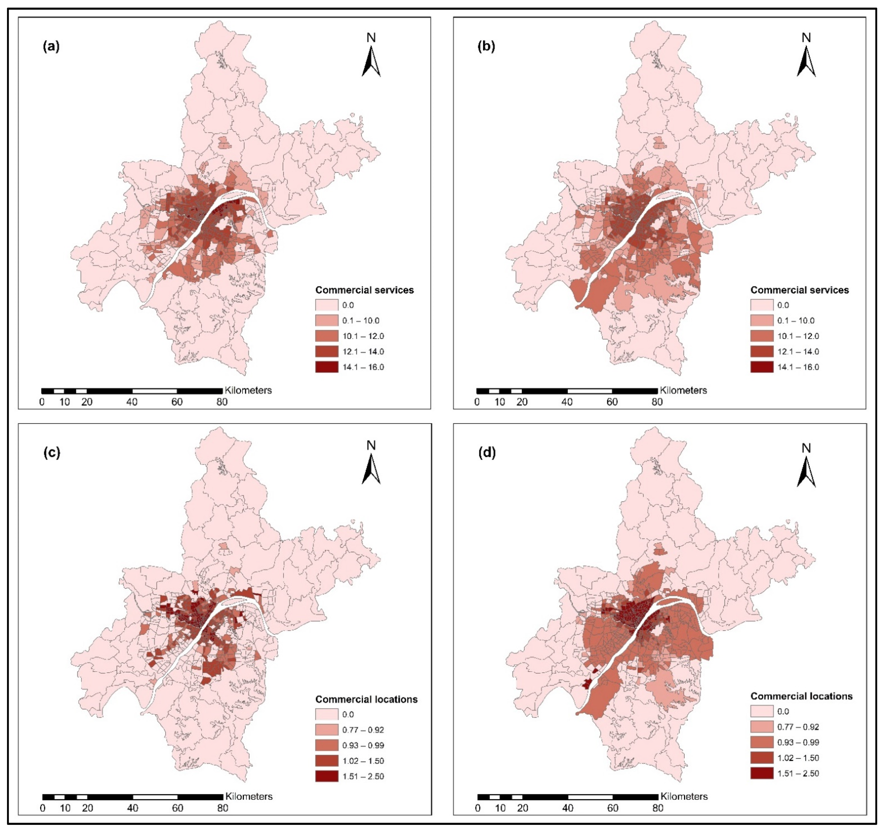
Figure 15a,b presents the results of bus accessibility to commercial services located within the study area. In 2015, new bus lines introduced were added, which eventually provided bus accessibility to a wider area. Results revealed that during 2015, the AIs increased significantly, and most of the AI values are in the range 10–14. Figure 15a,b indicates the range of bus accessibility values for commercial activities for 2012 and 2015: no accessibility (0); low–medium accessibility (5~8); medium accessibility (8.1~10); medium–high accessibility (10.1~12); high accessibility (12.1~14).

Meanwhile, the ISE-estimated commercial location using bus-dependent accessibility during the years 2012 and 2015 is presented in Figure 15c,d. The results revealed that areas with a high level of bus accessibility to commercial services showed a high level of commercial locations, especially during the year 2015. The CLI ISE-estimated commercial locations ranges are as follows: no commercial locations (0.0); low–medium level of commercial locations (0.77~0.92); medium level of commercial location (0.93~0.99); medium–high level of commercial locations (1.02~1.5); high level of commercial location (1.51~2.5).

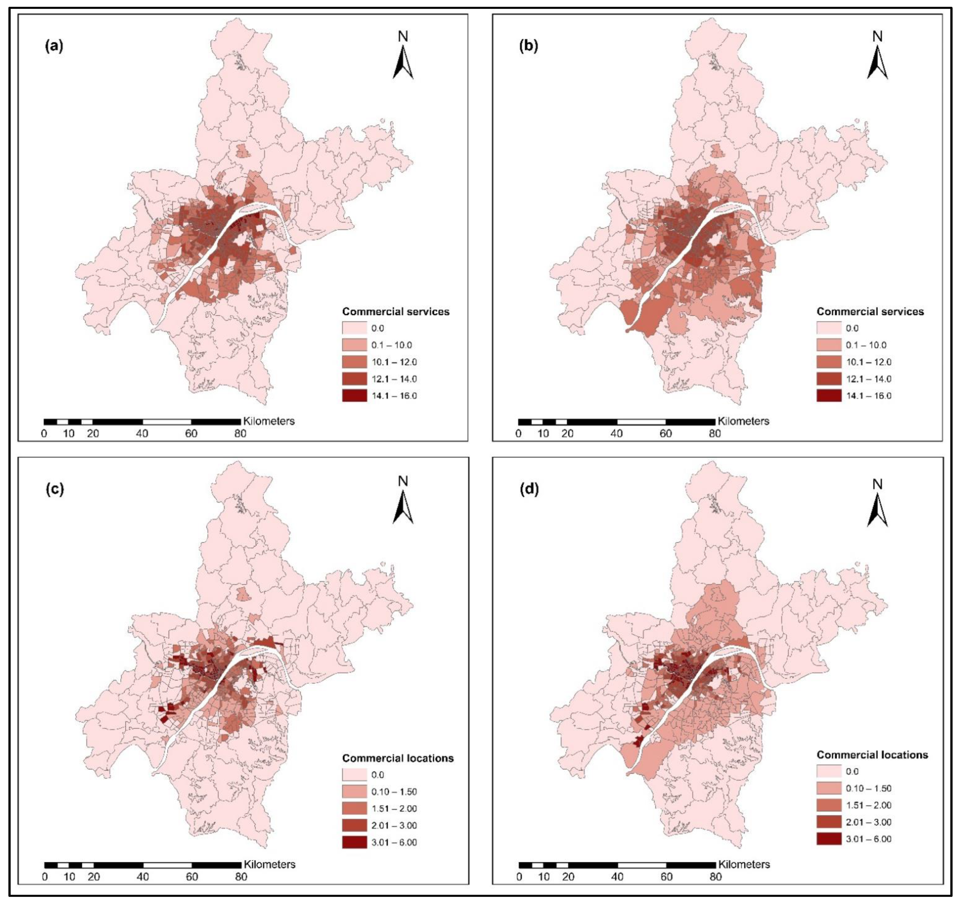
Accessibility to commercial services using transit as a combined mode is presented in Figure 16a,b for the years 2012 and 2015. Results indicated that areas with a high density of transit lines showed high transit accessibility to commercial services, especially during the year 2015, which was relatively high compared to 2012 because of new bus lines and metro lines introduced in the year 2015. Results revealed that during 2015, the AIs increased significantly. The range of transit AI to commercial activities in 2012 and 2015 were: low accessibility (0), low–medium accessibility (0.1~10), medium accessibility (10.1~12), medium–high accessibility (12.1~14), and high accessibility (14.1~16).

Meanwhile, the ISE-estimated commercial locations for the years 2012 and 2015 are presented in Figure 16c,d. Results revealed that areas with high transit accessibility to commercial services showed a high level of commercial locations estimated by the ISE model, and most of the CLI values were in the range 2.0–6. The results indicate the following: no commercial locations (0.0); low–medium level of commercial locations (0.1~1.5); medium level of commercial location (1.6~2.0); medium–high level of commercial locations (2.1~3.0); and high level of commercial location (3.1~6.0).

The ISE commercial services model activity locations results revealed that commercial services were susceptible to MDA rather than static accessibility measure.

5.2. Discussion

Accessibility plays a vital role in the social and environmental aspects. The impact of location rents is poorly known. Activities tend to be located close to high accessibility locations (which in turn influences rents as well). However, it is crucial to understand the actual effect of MDA on location choice behavior of activities and decisions of where to live, where to shop, and where to work. The MDA index provides a synthetic measurement of the ability to reach a particular type of opportunity within a specific time from a place of origin to a specific destination over time and space. Thus, accessibility is defined as a measurement of the capacity to communicate between human activities or settlements using a determined transport system. The usual measurement units are distance, time, mode, and the number of opportunities (activities) available at the destination. These opportunities include jobs, services, etc.; accessibility measures represent the impact that land use distribution and transport systems have on users. It indicates that both concepts, land use and transport, should be related because they allow individuals to participate in activities that take place in different locations. The utility of purchasing a commodity will influence the location utility of an activity that consumes a substantial amount of that commodity.

To understand and distinguish the location choice of various activities, the following two models are developed using ISE models: (i) Household activity location model; (ii) Commercial services activity location model. Location choice behavior of household activities depends on the nature of employment type and access to specific employment locations by a specific time of the day using specific modes. The location preference of household activities may vary depending on the household decision. Working households with no other priorities preferred location, which is within the range of adequate transport accessibility by a specific mode to their job location.

The ISE results revealed that urban households living in the downtown area of the City of Wuhan were sensitive to MDA offered by transit. It also revealed that urban households in the year 2015 showed high household activities estimated by transit-based ISE. This means urban households living in the downtown area are susceptible to MDA offered by the transit system. The results indicated that commercial activities were sensitive to MDA using transit during the years 2012 and 2015. Meanwhile, in the year 2015, when the new transit routes were added and improved the transit accessibility to commercial activities, it was found that commercial activities relocate to a location that offers high transit accessibility. The results also indicated that location decisions of commercial activities are influenced by MDA offered by transit. Nevertheless, the results indicate that commercial and household activities prefer locations with high accessibility offered by different modes.

The static and ISE–MDA models result revealed that household and commercial activities prefer locations that offer high MDA rather than the static accessibility offered, as shown in

Table 7. Comparison between static and ISE–MDA models.

	Static Logsum Model (R2)	ISE–MDA (R2)
Activities	Combined-Mode	Auto	Bus	Metro	Transit
Households	0.727	0.793	0.642	0.642	0.845
Commercial	0.485	0.842	0.530	0.698	0.905

. The auto-based ISE–MDA showed an R² value of 0.793, and the R² value for the static model was lower than 0.727. Meanwhile, transit-based ISE–MDA showed an R² value of 0.905 for commercial services, while the static logsum model showed an R² value of 0.485. The ISE–MDA models result indicates that location choice behavior of activities has a strong relationship with MDA and has weak relation or causal relationship with static accessibility models. The behavior point, the combined mode (all modes), is not usually considered when choosing the location. Instead, activities are sensitive to specific modes. It is concluded that MDA and ISE models affect the location choice behavior of activities rather than the static logsum models. Hence, for long-term and short-term urban planning exercises, planners and policymakers should consider MDA rather than static logsums.

6. Conclusions

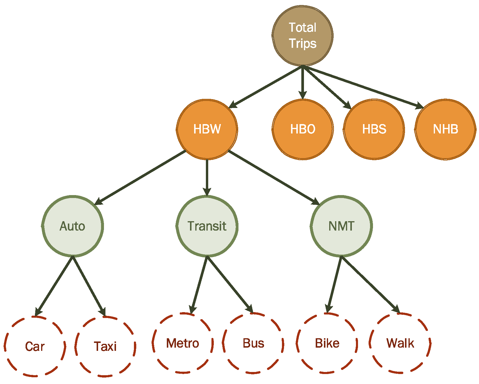
This study analyzed the impact of short-term spatial accessibility through Mode-Dependent Accessibility (MDA) on the location choice behaviors of urban activities such as households and commercialin the City of Wuhan, China. This study used auto (private cars and taxis) and public transit (metro, and bus) for measuring MDA. To comprehensively capture accessibility and location choice behaviors of urban activities, this study explicitly analyzed the effects of the metro and bus, as well as their combined effects. The current study used the data from the years 2012 and 2015. These data sets contained household travel survey data, transportation network, transit network, mobile phone signals, and land use data used to develop the land use and transportation interaction model. The study employed the M-TDM model to measure the impact of short-term MDA on household and commercial activities for the years 2012, and 2015. In addition, an advanced integrated spatial economic (ISE) models, i.e., PECAS (Production, Exchange, Consumption, Allocation, System) in order to investigate location preferences of urban activities over space and time. The PECAS approach imitates the spatial economic systems under consideration and has been improved with several distinct features such as an improved representation of socioeconomic systems through a social accounting matrix and microsimulation-based space development. Although locational model methodologies are based on a variety of attributes or characteristics, they all share a common theoretical background based on the random utility theory maximization. Moreover, location models do not function in an isolated way; rather, they are integrated into larger modeling systems such as land use—transport interaction (LUTI) modeling. It is crucial to recognize that the location selection of activities has a strong relationship with the transport system and is influenced by mode-specific accessibility. Accessibility is a dynamic feature of locations that varies in time and mode due to the changes in the transport network and changing patterns of activity distribution at different times of the day.

This study’s contribution was to evaluate the short-term MDA for the locational preference of household and commercial urban activities, which could help to capture the effect of MDA under diverse temporal and transport network impedance conditions on the location choice of urban activities. However, the traditional accessibility parameters do not adequately account for the short- and long-term requirements of urban activities. Therefore, it is crucial to create a solution that might provide a more effective planning tool for a thorough understanding of the urban system. This study examined the dynamic short-term accessibility of urban activities, which could be a more effective planning tool than typical “static” accessibility terms. Regarding household and commercial location choice, the ISE modeling results revealed that households and commercial activities are sensitive to MDA, especially using transit. In addition, their findings suggest that highly accessible locations that are well served by automobiles are more appealing for household and commercial activities. The ISE model results estimated that household and commercial location choice models show R² of 0.84–0.90 for transit-based accessibility, whereas the logsum-based static models show R² of 0.48–0.72. These results from the ISE models revealed that there was a strong relationship between the MDA and the location choice behavior of urban activities.

This study contributes to the existing body of literature with insightful findings, but there are a few limitations that must be acknowledged. This study assessed the short-term MDA for locational preference behaviors for urban activities. However, future studies should examine MDA over various time periods. The current study did not account for nonmotorized modes, which do not affect congestion time but can affect the accessibility of the first and last miles. Future studies must include nonmotorized modes to comprehensively capture the location choice behaviors. It is believed that data limitations pose the greatest hindrance to the development of such a complex model, especially in developing countries, because it requires large data sets such as economic and demographic data, household travel data, real state data, rent, occupancy, floorspace data, AADT, and mobile phone signal data. Due to the lack of self-reported travel data in developing countries, it is recommended that a survey is conducted to collect the necessary recent data for the model, which may yield useful findings. As time progresses, developments in information technology have provided new opportunities for data and tools to extract the required data. Our forthcoming research aims to address the above inadequacies when the necessary and most current data becomes available.