An Intelligent Homogeneous Model Based on an Enhanced Weighted Kernel Self-Organizing Map for Forecasting House Prices

Abstract

Accurately forecasting housing prices will enable investors to attain profits, and it can provide information to stakeholders that housing prices in the community are falling, stabilizing, or rising. Previous studies on housing price forecasting mostly used hedonic pricing and weighted regression methods, which led to the lack of consideration of the nonlinear relationship model and its explanatory power. Furthermore, the attribute data of housing price forecasts are a heterogeneous study, and they are difficult to forecast accurately. Therefore, this study proposes an intelligent homogeneous model based on an enhanced weighted kernel self-organizing map (EW-KSOM) for forecasting house prices; that is, this study proposes an EW-KSOM algorithm to cluster the collected data and then applies random forest, extra tree, multilayer perception, and support vector regression to forecast the house prices of full, district, and apartment complex data. In the experimental comparison, we compare the performance of the proposed enhanced weighted kernel self-organizing map with the listing clustering methods. The results show that the best forecast algorithm is the combined EW-KSOM and random forest under the root mean square error and root-relative square error, and the proposed method can effectively improve the forecast capability of housing prices and understand the influencing factors of housing prices in full and important districts. Furthermore, we obtain that the top five key factors influencing house prices are transferred land area, house age, building transfer total area, population percentage, and the total number of floors. Lastly, the research results can provide references for investors and related organizations.

1. Introduction

Housing is a basic human need, and everyone needs a place to live. Real estate is both a consumer product and an investment product [1], and it also has a significant impact on macroeconomics. Housing allocation is increasingly important for sustainable economic development and social stability because it is related to people’s lives, and the demand for residential land is also an important issue in real estate [2]. House price appraisal is one of the most important transaction decisions that affects the national real estate policy [3]. Hence, the stakeholders use various information about a house to measure the value-to-price ratio of it. Housing prices are affected by many factors, including the market economy, industrial policies, land price, income levels in different regions, living environment, public facilities, and the needs of the people [4]. Furthermore, the changes in housing prices cover various influencing factors, and important factors can be obtained through data analysis. Stakeholders understand how real estate buyers and sellers evaluate housing prices and produce better evaluation indicators, and then the government can propose corresponding policies to maintain the stability of the real estate market, including adjusting the land supply structure and buying houses.

Many people have expressed widespread concern about housing prices, and an effective tool for forecasting future housing price fluctuations is needed. Various methods have been applied to forecast housing prices. Multivariate statistical models can consider many factors that affect housing prices. However, they require some assumptions on data distribution, and the performance of these models is easily limited by sample size and data integrity. Compared with statistical models, intelligent forecast models are now becoming mainstream because they can identify the nonlinear relationship between variables and provide higher accuracy and deeper interpretation of the behavior of market interaction. The cost and efficiency of intelligent learning from external data and economic signals are no longer an obstacle, and more and more stakeholders are adopting intelligent predictions to forecast housing prices.

The data of housing price forecasts are part of a heterogeneous study. The most obvious heterogeneity of housing prices is that relatively low-priced properties are more likely to find buyers than those with higher prices. For an inexperienced agent, for a price higher than the inferred price, the price increase leads to a greater decrease in the probability of sales compared with a price lower than the inferred price. For any price, the more experienced agents are more likely to sell. It is very difficult to forecast housing prices correctly. However, we can use a large amount of collected data to reduce the forecast error by using the method of homogenizing the data, such as how a clustering algorithm can group heterogeneous data into similar clusters. Therefore, this research proposes an enhanced weighted kernel self-organizing map (EW-KSOM) to cluster the collected attribute data of real estate transactions and to forecast housing prices by using four intelligent models. The following are the contributions of this research:

• Collect data from the real price registration of real estate information in Taiwan and the population statistics data from the Civil Affairs Bureau of the Taichung City government. The originally collected data have a total of 16,617 records with 26 attributes. It is also found from the relevant literature that the collected data have 12 important attributes that affect the changes in housing prices.
• Use the proposed EW-KSOM to cluster the collected data and then compare it with the listing clustering algorithms.
• Apply random forest, extra tree, multilayer perception regression, and support vector regression to forecast the house prices of full and important districts, and we compare the performance of the proposed intelligent homogenous model with the listing methods.
• The results can be used as references for home buyers, real estate companies, and relevant government agencies.

The remaining sections of this paper are organized as follows. Section 2 introduces the related work, including the factors and forecasts of real estate prices, clustering techniques, and intelligent forecast methods. The proposed method and computational steps are described in Section 3. Section 4 explains the dataset and experimental environment. Section 5 illustrates the experimental results and comparisons. Section 6 presents the discussions, and Section 7 presents the conclusion.

2. Related Work

This section introduces the factors and forecasts of real estate prices, clustering techniques, and intelligent forecast methods.

2.1. Forecasts and Factors of Real Estate Prices

The research trend of real estate price forecasting in the past 10 years is based on hedonic regression and artificial intelligence methods to forecast real estate prices [3]. The location choice of dwellings and real estate prices are concerns of the public, and the location choice of buyers will affect real estate prices. These forecasting methods of real estate prices include spatial regression and hedonic models [5]. Kumar et al. [6] performed regression analysis on real estate prices based on various attributes of the residence (such as the number of rooms, bathrooms, and other attributes) to forecast future prices. Previous studies on housing prices are mostly based on the hedonistic method, which is a traditional statistical estimation method. The hedonic price model developed by Rosen [7] and its implicit prices can be derived from attributes that constitute goods or services. The hedonic price regression aims to select the living environment indicators based on the price that people are willing to pay in the living environment and use regression analysis to explore the relationship between the value of the real estate and the related attributes. The spatial regression method obtains spatial dependence in regression analysis, which avoids unstable statistical parameters and unreliable significance tests and provides information about the spatial relationship between variables. Taltavull de La Paz et al. [8] showed that there is a spatial autocorrelation between housing prices in the local market, and spatial factors also affect the growth of housing prices. Therefore, the spatial regression model can be applied to explore the influence of residential spatial factors on housing prices.

Park and Bae [3] pointed out that machine learning algorithms can improve housing price forecasts and compare the performance of various classifiers. Truong et al. [9] used various machine learning techniques to provide optimal results for housing price forecasts, and the results showed that random forest has the lowest error on the training dataset. Random forest can be used to explore the relationship between housing prices and their factors for helping to determine important attributes and forecast housing prices [10]. Rico-Juan and Taltavull de La Paz [11] used random forest and hedonic regression to evaluate the accuracy of housing price forecasts, and their results showed that the combination of technologies would increase the information about the nonlinear relationship between housing prices and housing attributes in the real estate market. Furthermore, Kumar et al. [6] used k-means to determine the central location of the house landmark and then selected the cluster closest to the household’s preference to select the best apartment. Furthermore, Kang et al. [12] used a deep learning model to extract features from street view images and house photos, and they used a machine learning model and two spatial scales of geographically weighted regression to establish a housing price model. The results showed that their framework could model the housing price appreciation with high accuracy.

According to a 2016 survey conducted by the National Association of Realtors, one-third of home buyers are first-time home buyers, and two-thirds are experienced home buyers [1]. Therefore, the vigorous development of the real estate industry has been regarded as an important economic industry and having a high degree of correlation with economic driving forces [2]. From an economic perspective, the potential factors affecting housing prices include four dimensions: structure (size, age, and decoration of a house), neighborhood (school, hospital, and parks), location (city center), and landscape. The location of the real estate in the city is one of the important factors, and it will affect the pricing standard for the best location [6,13]. Debrezion et al. [14] illustrated the positive impact of railway accessibility on housing prices from the sales data of three metropolitan areas in the Netherlands. We list some important housing price factors and methods in Table 1.

Table 1. Some important housing price factors and methods.

Factor	Method	Reference
Residential type	Multiple regression, principal component analysis, and vector autoregressive	Das et al. [1]
Population	Multiple regression and gradient boosting machine	Kang et al. [12]
Proximity to public facilities	Logistic regression	Shih et al. [15]
Living environment	Multiple regression	Tubadji and Nijkamp [16]
Location	Decision tree, principal component analysis, and k-means	Kumar et al. [6]
Floor of dwelling	Multiple regression	D’Acci [13]
The number of bedrooms	Multiple regression	D’Acci [13]
The number of bathrooms	Decision tree, principal component analysis, and k-means	Kumar et al. [6]
House age	Decision tree, principal component analysis, and k-means	Kumar et al. [6]
Building construction type	Decision tree, principal component analysis, and k-means	Kumar et al. [6]
Dining hall type	Decision tree, principal component analysis, and k-means	Kumar et al. [6]
Area of the house	C4.5, RIPPER, naïve Bayesian, and AdaBoost	Park et al. [3]

2.2. Clustering Techniques

Cluster analysis is a multivariate statistical method [17], and it involes the task of grouping data; that is, the data in the same clusters are more similar to the data in other clusters (e.g., the distance is closer). There are many clustering algorithms in the literature, such as k-means [18], kernel k-means [19], and self-organizing maps [20]. This section only introduces the relevant clustering algorithms used in this research, including k-means (KM), kernel k-means (KKM), self-organizing maps (SOMs), and kernel self-organizing maps (KSOMs).

1.

KM

KM is used to find outliers and group similar data groups, and it is a distance-based clustering algorithm. The smaller the distance to the object, the greater the similarity [21]. When the number of clusters is fixed to k, we find k cluster centers and assign the object to the nearest cluster center in order to minimize the squared distance from the cluster [22]. Determining the number of clusters is an important step in the KM clustering algorithm. We can use the elbow method [23] and the average silhouette method [24] to determine the number of clusters.

2.

KKM

The KM algorithm assumes that all data points are in a Euclidean space and that they cannot handle nonlinearly separable datasets. To solve this problem, the kernel is introduced into KM clustering [25], which is based on the kernel to cluster KM. It embeds data points in a high-dimensional nonlinear manifold and uses a nonlinear kernel distance function to define their similarity and capture the nonlinear structure in the dataset. KKM clustering can achieve a higher clustering quality than KM clustering, such as with a scalable KKM algorithm [26].

3.

SOM

SOM is unsupervised competitive learning developed by Kohonen [20], which performs clustering and nonlinear projection of datasets at the same time. SOM uses a set of neurons arranged according to a low-dimensional structure, and the original data are divided into as many homogeneous clusters as the model such that the close clusters contain close data points in the original space. The advantages of SOM are that it maps N-dimensional data to a two-dimensional space and keeps the topology of the data and it is not necessary to assign the number of clusters.

4.

KSOM

A kernel is a function which is a dot product operation of a high-dimensional feature space. MacDonald and Fyfe [27] proposed a k-means-based kernel SOM, and each mean is described as a weighted sum of the mapping function. Another KSOM is based on the normalized gradient descent method [28,29], and the algorithm aims to minimize the mean square error of the input and the corresponding prototype in the mapping space.

2.3. Intelligent Forecast Methods

1.

Random Forest (RF)

RF is a nonlinear computation method developed by Breiman [30] which is composed of many decision trees to solve regression and classification problems. RF is an ensemble learning method where when the number of trees increases, it can prevent overfitting. RF in regression is used to average the results of all independent trees, and the majority voting method is used to obtain the results in classification [31]. RF can handle both categorical and numerical variables in the forecast problem, and it can rank the importance of the variables from the most relevant to the least relevant for adding value to the attribute selection in data analysis [31,32].

2.

Extra Tree (ET)

ET is an ensemble learning algorithm, and it is an extension of the RF algorithm proposed by Geurts et al. [33]. ET increases the randomness of the RF algorithm, and it is very similar to RF in operation. The ET algorithm creates a series of original gradients or regression trees based on the traditional top-down procedure. The two main differences between ET and other tree-based methods are that it separates nodes by randomly selecting cut points and uses the entire learning sample to grow the tree. The ET algorithm increases randomization and the number of trees to control the stability of the performance and is immune to overfitting of the training dataset. Therefore, ET adds randomization but still has optimization to prevent overfitting and provide better performance [33,34].

3.

Multilayer Perceptron (MLP)

MLP is an artificial neural network which is basically composed of three layers: the input, hidden, and output layers. It is a feedforward neural network, and the neurons are connected together from the input layer to the hidden layer and finally to the output layer [35]. MLP uses the backpropagation method to adjust the error and weight of the network [36]. The error is generated by the neuron in the output layer, and the error is feedback. Finally, the weight is adjusted, and the process is repeated until the error is minimized. MLP uses activation functions and backpropagation methods to achieve a good learning model, and it is a nonlinear model with better fault tolerance. MLP can be used in regression forecast problems, namely MLP regression (MLPR), such as how Bin et al. [37] used MLP to build a real estate appraisal model which could find a more accurate forecast of house prices.

4.

Support Vector Regression (SVR)

SVM is a supervised learning algorithm for classification and regression forecasting developed by Vapnik et al. [38]. SVM is used for classification problems, called support vector machine (SVM), while in regression problems, it is called SVR. The main purpose of SVR is to find the best separating hyperplane to separate the clustered data, and it can solve a nonlinear problem. SVM can handle high-dimensional attributes for classification, but the disadvantage is that it will be very inefficient for a large number of samples and very sensitive to missing data. In addition, SVM needs to find suitable kernel functions, such as linear, polynomial, sigmoid, and radial basis functions. In the SVR application, Kamara et al. [39] used deep learning models, including SVR, to solve the forecast of the number of days on sale, and their results provide sellers the ability to adjust their prices in response to expected sales.

3. Proposed Model

This section introduces the proposed EW-KSOM and intelligent homogeneous model based on the EW-KSOM algorithm.

3.1. EW-KSOM Algorithm

Hung [40] applied k-means to cluster the heterogeneous data into the homogeneous data and presented a homogeneous attribute intelligent model for forecasting house prices. MacDonald and Fyfe [27] proposed a k-means-based KSOM, where each mean is described as a weighted sum of the mapping function. Based on the gradient descent method, Andras [29] proposed a kernel-Kohonen network, where the input and weights are transformed into the high-dimensional kernel Hilbert space. The Euclidean distance in the high-dimensional space is the updated weight. Another KSOM is also based on the normalized gradient descent method [28], in which the algorithm aims to minimize the mean square error of the input and the corresponding prototype in the mapping space. The SOM and KSOM are not necessarily assigned the number of clusters in advance. After training the weight coefficients by competitive learning, the center of each cluster is automatically obtained. Furthermore, Lau et al. [41] stated that these kernel extensions of the original SOM are to minimize the energy function, and a KSOM can provide slightly better performance than other methods. To enhance the clustering capability and reduce heterogeneity, this study proposes an EW-KSOM algorithm. First, we set the objective and enhanced the weighted function. Let i(X) be the index of the winning neuron with respect to the input X. Hence, the objective function is

$$i\left(X\right)=\arg \min E_w\left(j\right)\left|\right|X-W_j\left|\right|{}^2$$

(1)

The weighted function is E_w(j) = exp(−‖X − W_j‖²/σ²), and the parameter σ = [0.1,1].

Second, the EW-KSOM algorithm is as follows:

1.

Define the input and output layer.

Assuming that an input dataset is X’ = [x₁, x₂, x₃ … x_n], which is an n-dimensional vector, and the number of neurons in the input layer is n. The neurons in the output layer are arranged in a matrix in a two-dimensional space, and each neuron has a weight vector.

2.

Normalize the input vector and weight:

$$X=X^{\prime }/\left|\right|X\left|\right|$$

(2)

$$w_j=W_j/\left|\right|W\left|\right|$$

(3)

where ‖X‖ and ‖W‖ are the Euclidean norms of the input and weight vector, respectively.

3.

Input the data into the neural network.

Use the dot product to calculate the normalized data and weight vector. The output neuron with the largest dot product value wins the competition.

4.

Update the neurons in the topological neighborhood of the winning neuron.

The updating weight of the winning neuron is

$$w_j(t+1)=w_j\left(t\right)+E_w\left(j\right)\eta \left(j\right)h_j\nabla J\left(w_j\right)$$

(4)

where J(w_j)= ‖φ(X’) − φ(w_j)‖² = 2w_j − 2φ(X’), φ is a kernel function, ∇ is gradient descent, η(j) is the learning rate function of the training step j, and the topological distance from the winning neuron is defined.

Furthermore, the winning neighborhood function is

$$h_j=\exp \left(-\frac{d}{2{\delta }^2\left(j\right)}\right),$$

(5)

where δ(t) = d × (j_max − j)/j_max is the width of the topological neighborhood function, d = ‖r_i(x) − r_j‖², r_j is the location of neuron j, and r_i(x) is the location of winning neuron.

5.

Update the learning rate.

Change the different learning rate η and the topological neighborhood N, and η(j) = 1/j generally takes the reciprocal of the number of iterations. When N increases, the time and the distance decrease.

6.

Determine whether to converge.

If the learning rate η ≤ η_min or reaches the set number of iterations, then the algorithm ends.

3.2. Intelligent Homogeneous Model Based on the EW-KSOM Algorithm

The data of housing price forecasts are a heterogeneous study, and it is difficult to accurately forecast housing prices because there are many different data sources, including the category and numeric value. This study referred to Hung [40], who applied k-mean to cluster the heterogeneous data into the homogeneous data for improving housing price forecasting. Therefore, we proposed an EW-KSOM algorithm to cluster the collected data and named each cluster. Furthermore, we applied RF, ET, MLPR, and SVR to forecast the house prices of full and important districts, and we compared the performance of EW-KSOM with the listing clustering methods. The procedure of the proposed intelligent homogeneous model based on EW-KSOM for forecasting house prices is shown in Figure 1. The procedure contained five steps: data collection, data preprocessing, the proposed EW-KSOM algorithm, forecasting house prices, and evaluation and comparison. Steps 1 and 2 are described in Section 4, and steps 3 and 4 are explained in this section. Here, we only introduce the root mean square error (RMSE) and root relative squared error (RRSE) of step 5 as follows.

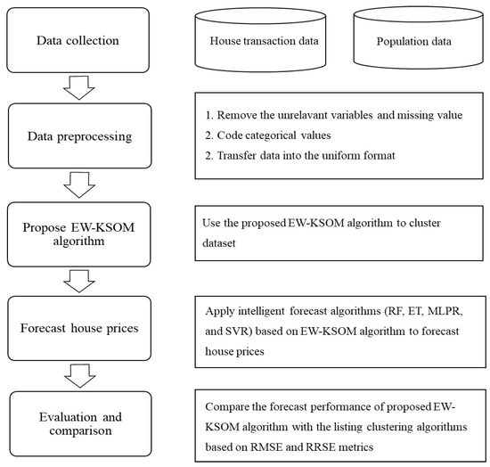
Figure 1. Procedure of intelligent homogeneous model based on EW-KSOM for forecasting house prices.

1.

RMSE

RMSE represents the sample standard error of the difference between the forecasted value and the observed value [42]. The RMSE is mainly used to aggregate the size of the error in the forecast with a value to show its forecast ability. The RMSE is a good measure of accuracy, but because it is related to the numerical range, it can only be used to compare the forecasted error of a specific variable between different models. The RMSE is defined as shown in Equation (6):

$$\mathrm{RMSE}=\sqrt{\frac{{{\displaystyle \sum }}_{i=1}^n{\left|T\left(i\right)-F\left(i\right)\right|}^2}{n}}$$

(6)

where T(i) represents the actual house prices, F(i) denotes the forecasted house prices, and n is the amount of data.

2.

RRSE

RRSE [43] takes the total square error and normalizes it by dividing the total square error of the actual values. By taking the square root of the relative square error, the error can be reduced to the same dimension as the forecasted amount. It is defined as shown in Equation (7):

$$\sqrt{{\displaystyle \sum }_{i=1}^n{\left|T\left(i\right)-F\left(i\right)\right|}^2/{\displaystyle \sum }_{\mathrm{i}=1}^{\mathrm{n}}{\left|T\left(i\right)-\overline{T\left(i\right)}\right|}^2}$$

(7)

where $\overline{T\left(i\right)}={\displaystyle \sum }_{i=1}^{n}T\left(i\right)/n$.

4. Dataset and Experimental Environment

Taichung City has a population of about 2.82 million and is the second-most populous city in Taiwan. Taichung City has 29 administrative districts, but the Heping and Daan districts have no house transaction records. Therefore, the collected data contained 27 administrative districts of Taichung City from the real price registration of real estate information in Taiwan (https://pip.moi.gov.tw/V3/Z/SCRZ0211.aspx?Mode=PN02 (accessed on 1 March 2021)), and the population statistics data were from the Civil Affairs Bureau of the Taichung City government (https://demographics.taichung.gov.tw/Demographic/index.html?s=12685860 (accessed on 1 March 2021)). The original data were collected from real estate registration data from 2019 to 2020, and we selected the residential transaction data with 26 attributes and 16,617 records. This study used the population percentage of 29 administrative districts and the average house prices (TWD/m²) in Taichung City to express the impact of community environment and economic development on housing prices, as shown in Table 2. After preprocessing, the retained attributes included the district population percentage, transfer floor, total floor, building construction type, house age, transferred land area, total area square meters of building transfer, bedroom, living room, bathroom, compartmented, management, and unit price per square meter. Then, we coded these categorical variables as digital for clustering and forecasting, and the descriptions and values of the 12 independent variables and 1 dependent variable (house prices) are shown in Table 3.

Table 2. The 29 administrative districts and average house prices in Taichung City.

District	Population Percentage (%)	The Number of Transactions	Transaction Percentage (%)	Average House Prices (Taiwan Dollars/m2)
Beitun	10.29	2954	18.51	59,495.57
Xitun	8.21	3349	20.99	65,704.80
Dali	7.54	249	1.56	64,986.94
Taiping	6.94	208	1.30	81,757.73
Nantun	6.27	2037	12.77	68,130.58
Fengyuan	5.87	538	3.37	54,178.21
North	5.15	2285	14.32	56,040.20
South	4.49	914	5.73	50,818.44
West	4.03	1045	6.55	59,443.05
Tanzi	3.87	604	3.79	52,382.98
Daya	3.40	258	1.62	49,804.59
Shalu	3.39	238	1.49	49,960.79
Qingshui	3.14	148	0.93	43,729.76
Longjing	2.77	210	1.32	44,988.53
Wuri	2.73	72	0.45	64,658.75
Dajia	2.69	98	0.61	42,124.94
East	2.68	267	1.67	51,379.72
Shengang	2.31	87	0.55	47,095.86
Wufeng	2.30	38	0.24	54,687.49
Wuqi	2.11	75	0.47	53,980.48
Dadu	2.01	76	0.48	36,590.17
Houli	1.92	60	0.38	56,764.40
Dongshi	1.73	75	0.47	35,527.01
Waipu	1.13	18	0.11	34,527.22
Xinshe	0.85	8	0.05	36,796.75
Daan	0.66	0	0	N/A
Central	0.63	40	0.25	36,400.72
Shigang	0.51	4	0.03	36,313.00
Heping	0.38	0	0	N/A

Note: Taichung’s population is 2,818,139, and the total number of transactions was 15,955.

Table 3. Operational definitions of the dependent and independent variables.

Variable	Description	Value
Population percentage	Population percentage of 29 administrative districts in Taichung City	Numeric value
Transfer floor	Transaction floor status: “0” denotes full floor, “i” represents transfer the i-th floor	Categorical value: 0, 1, 2… 22.
Total number of floors	The total number of floors in this house	Categorical value: 1, 2… 38.
Building construction type	Housing type: “1” denotes a small studio apartment, “2” represents an old condominium (below five floors and no elevator), “3” denotes house (townhouse, villa, mansion), “4” represents apartment complex (below 10 floors with elevator), and “5” means apartment complex (all floors with elevator)	Categorical value: 1, 2, 3, 4, and 5.
House age	The year and month of residential transaction minus the year and month of residential construction.	Numeric value
Transferred land area (m2)	The land area of the house	Numeric value
Building transfer total area (m2)	Building transfer total area	Numeric value
Bedroom	The number of bedrooms in the house	Integer value
Living room	The number of living rooms in the house	Integer value
Bathroom	The number of bathrooms in the house	Integer value
Compartmented	Does the house have compartments?	“1” denotes yes, and “0” means no
Management	Does the house have a housing management committee?	“1” denotes yes, and “0” means no
Unit price per square meter	Transaction price per square meter (Taiwan dollars)	Numeric value

To visualize the data, we used the Geocoding API of the Google Maps service to obtain the latitude and longitude based on the locations (address) of the transaction houses, and then we applied the Choropleth and HeatMap of map visualizations in the Python tool to generate visual maps. Figure 2 only shows the 27 administrative districts with transaction records, and it is a map visualization of the average house prices/m² for each district. The deeper color districts denote higher house prices. From Table 2 and Figure 2, we observe that the highest housing prices in the Taiping district were due to the new expressway (Taiwan Route 74), with convenient transportation close to the urban area, a large land area, and new residential buildings.

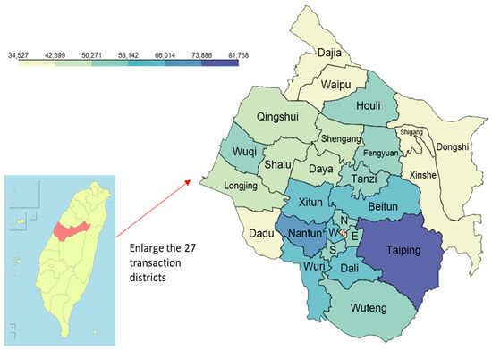
Figure 2. Average house price/m² for each district.

The experimental environment used Python 3.7.4 to compute all results and visualize data on an Intel i7-7700 with a Windows 10 operating system and a 3.6-GHz CPU. Four forecasting algorithms (RF, ET, MLPR, and SVR) were used to forecast the housing prices. The parameter settings of the clustering and forecast algorithms are shown in Table 4.

Table 4. Algorithms and their parameter settings.

Algorithm	Parameter	Reference
KM	n_clusters: k = 4, maxiteration = 500, and tolerance = 0.0001	Sinaga and Yang [18]
KKM	Kernel function: RBF, n_clusters: k = 4, maxiteration = 500, and tolerance = 0.0001	Dhillon et al. [19]
SOM	Dimension = 2, iterations = 3000, neighborhood: Guassian, topol shape: hexa and rect	Kohonen [20]
KSOM	Iterations = 3000, neighborhood: Guassian, kernel function: RBF	Pan et al. [28]
EW-KSOM	Iterations = 3000, neighborhood: Guassian, kernel function: RBF	Proposed
RF	Iterations = 100, batch size = 100	Breiman [30]
ET	Iterations = 10, batch size = 100	Geurts et al. [33]
SVR	Kernel function: RBF; epsilon = 0.001; gamma = 1/n (n is number of variables); C = 1	Cortes and Vapnik [38]
MLPR	activation function: sigmoid; loss function: square error; learning rate = 0.001; hidden layer sizes = 200	Relich and Świć [35]

5. Experimental Results and Comparisons

This section illustrates the proposed EW-KSOM algorithm to cluster the collected data and then applies RF, ET, MLPR, and SVR to forecast house prices. Furthermore, we compare the performance of the proposed enhanced weighted kernel self-organizing map with KM, SOM, KKM, KSOM, and no clustering algorithms. The experimental data was partitioned into 66% for training and 34% for testing, and the average of repeated implementation 100 times was taken to present their results for finding the best algorithm. After data preprocessing, we followed steps 3–5 of the proposed procedure in Figure 1 of Section 3.2. First, this experiment used the SOM family algorithms because the SOM, KSOM, and EW-KSOM do not need to assign the number of clusters in advance, and then the best number of clusters was four from the SOM family algorithms. Second, we implemented KM family algorithms based on the best number of clusters k = 4, and then we applied RF, ET, MLPR, and SVR to forecast house prices. The comparative results of the full data are shown in Table 5, and it shows that the proposed EW-KSOM algorithm combined with RF was the best forecast result in terms of the RMSE and RRSE metrics.

Table 5. Forecast results of different clustering methods.

Metric	Method	Cluster	RF	ET	MLPR	SVR
RMSE	SOM	Cluster_0	8635.49	9093.29	11,452.97	11,874.24
		Cluster_1	39,250.37	40,342.30	58,133.15	46,796.35
		Cluster_2	8473.34	8884.66	12,011.54	10,951.73
		Cluster_3	9105.38	9577.47	11,889.33	12,264.61
		Mean	16,366.15	16,974.43	23,371.75	20,471.73
	KM	Cluster_0	38,337.52	40,936.52	59,874.59	46,798.05
		Cluster_1	9156.01	9766.18	12,915.27	12,706.98
		Cluster_2	8548.91	9089.44	11,476.57	10,512.94
		Cluster_3	8631.88	9119.04	14,483.75	11,830.69
		Mean	16,168.58	17,227.80	24,687.55	20,462.17
	KSOM	Cluster_0	8635.49	9093.29	11,452.97	11,874.24
		Cluster_1	39,250.37	40,342.30	58,133.15	46,796.35
		Cluster_2	8473.34	8884.66	12,011.54	10,951.73
		Cluster_3	9105.38	9577.47	11,889.33	12,264.61
		Mean	14,207.27	16,974.43	23,371.75	20,471.73
	KKM	Cluster_0	7421.88	7773.32	10,283.38	9818.09
		Cluster_1	59,165.89	64,166.71	12,1929.04	73,348.07
		Cluster_2	80,135.18	86,157.62	13,4955.38	83,812.93
		Cluster_3	7496.00	7966.27	8397.17	8295.41
		Mean	38,554.74	41,515.98	68,891.24	43,818.63
	EW-KSOM	Cluster_0	29,146.84	31,800.90	64,375.41	37,768.25
		Cluster_1	5898.41	6159.44	6809.36	6684.28
		Cluster_2	6111.40	6461.76	7895.54	7085.51
		Cluster_3	9488.51	9978.76	14,927.50	12,803.43
		Mean	12,661.29	13,600.26	23,501.95	16,085.37
	No clustering		22,547.16	24,212.59	33,442.44	30,682.63
RRSE	SOM	Cluster_0	66.84	70.40	88.64	91.89
		Cluster_1	67.07	69.10	100.68	80.32
		Cluster_2	56.52	59.27	80.15	73.06
		Cluster_3	66.89	70.39	87.42	90.18
		Mean	64.33	67.29	89.22	83.86
	KM	Cluster_0	69.14	73.87	109.10	84.75
		Cluster_1	65.71	70.12	92.85	91.10
		Cluster_2	58.39	62.09	78.44	71.81
		Cluster_3	56.66	59.86	95.10	77.65
		Mean	62.48	66.49	93.87	81.33
	KSOM	Cluster_0	66.84	70.40	88.64	91.89
		Cluster_1	67.07	69.10	100.68	80.32
		Cluster_2	56.52	59.27	80.15	73.06
		Cluster_3	66.89	70.39	87.42	90.18
		Mean	64.33	67.29	89.22	83.86
	KKM	Cluster_0	74.51	78.04	103.19	98.56
		Cluster_1	95.73	104.14	190.42	119.51
		Cluster_2	90.75	98.77	159.11	90.39
		Cluster_3	85.41	90.77	95.69	94.52
		Mean	67.97	92.93	137.10	100.75
	EW-KSOM	Cluster_0	60.60	66.47	136.19	79.00
		Cluster_1	42.32	44.21	48.91	47.98
		Cluster_2	38.34	40.54	49.60	44.46
		Cluster_3	53.85	56.72	84.46	72.58
		Mean	48.78	51.99	79.79	61.01
	No clustering		64.62	69.64	95.37	88.37

Note: The bold digits denote the lowest error among the combined five clustering algorithms and four forecast methods in RMSE and RRSE metrics.

To further compare the performance of the proposed EW-KSOM algorithm, we chose the Beitun and Xitun districts, having the largest population and transaction volumes, to forecast house prices. In addition, the Xitun district is the location of the Taichung City government and council, being the most prosperous commercial area. From the comparative results of the full data in Table 5, we only used RF to forecast the house prices of the Beitun and Xitun districts. The results are shown in Table 6, and they show that the forecast capability of the proposed EW-KSOM was better than the listing methods (including no clustering) in terms of the RMSE and RRSE metrics. Furthermore, KKM was the worst clustering method, with results poorer than no clustering.

Table 6. District forecast results of proposed clustering and no clustering.

District	Metric	No Clustering	KM + RF	KKM + RF	SOM + RF	KSOM + RF	Proposed + RF
Beitun	RMSE	17,084.58	21,061.82	31,480.37	20,388.58	11,269.03	11,121.00
	RRSE	56.18	60.83	86.74	60.41	50.97	50.33
Xitun	RMSE	33,350.05	28,101.78	54,364.43	25,409.79	14,667.85	14,288.89
	RRSE	68.25	66.70	83.08	64.34	50.75	50.27

Note: The bold digits denote the lowest error among proposed clustering and the listing methods in RMSE and RRSE metrics.

6. Discussions

From the experimental results, the proposed EW-KSOM clustering algorithm was better than the listing algorithms based on the minimum RMSE and RRSE metrics. However, there are some findings and discussions, which are listed below:

1.

Key Factors

This study collected 13 factors (as Table 3) to forecast house prices, among which the population percentage was applied to express the importance of the geographical location of the region and its urban development. After the experimental results, we used the RF forecast model to rank the factors’ importance of full data, as shown in Figure 3. We observed that the top four positive factors are the following: transferred land area > house age > population percentage > total number of floors. The top four negative factors are as follows: building transfer total area > bedroom > living room > compartment. Our results are consistent with some literature: (1) housing prices in geographical locations with a large population would rise sharply [3,11], (2) the values of residential buildings on higher floors were relatively higher and has a positive impact [44], and (3) the house area was highly correlated with the house price [12]. Furthermore, we used apartment complex data (building construction type 5: all floors with the elevator, as in Table 3) from the collected data and ranked the factors’ importance of the apartment complex data, as shown in Figure 4. We observed that the four positive factors were the following: population percentage > building transfer total area > total number of floors > transfer floor. The top three negative factors were the following: house age > transferred land area > bedroom.

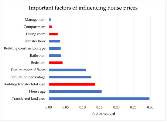
Figure 3. Important factors of influencing house prices (full data). Note: the blue bars denote positive factors, and the red bars mean negative factors.

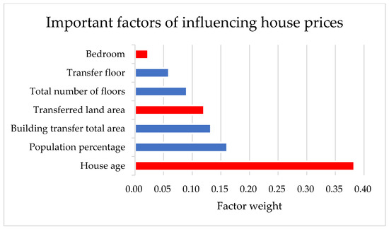
Figure 4. Important factors of influencing house prices (apartment complex data). Note: The blue bars denote positive factors, and the red bars mean negative factors.

2.

Homogeneous Effect

To improve forecast capabilities, this study proposes an intelligent homogeneous model based on EW-KSOM clustering to forecast house prices. The results show that the proposed EW-KSOM algorithm combined with RF had the best forecast results in the full and district data, as shown in Table 5 and Table 6. Furthermore, Kumar et al. [6] used k-means clustering to identify the locations of real estate investment based on user preferences and selected condominium and apartment complex data to rank the influencing factors of an apartment complex. Therefore, we also selected apartment complex data from the collected data and applied the proposed intelligent homogeneous model based on EW-KSOM clustering to forecast house prices. Here, we only compared the proposed algorithm with KSOM because the proposed EW-KSOM algorithm is a modified form of KSOM clustering. The results show that the proposed EW-KSOM algorithm combined with RF produced the best forecast result, as shown in Table 7. In summary, the clustering allowed the data to be homogeneous, the forecast effect was better than no clustering, and the proposed method was better than the listing methods.

Table 7. District comparison results of proposed clustering with no clustering.

Data	Metric	Cluster	KSOM + RF	EW-KSOM + RF
Apartment complex (floors with elevator)	RMSE	Cluster_0	7496.87	7460.05
		Cluster_1	5227.51	5361.11
		Cluster_2	5966.73	5928.15
		Cluster_3	7452.87	7194.46
		Mean	6536.00	6485.98
		No clustering		8225.22
	RRSE	Cluster_0	51.78	52.91
		Cluster_1	42.19	43.37
		Cluster_2	37.63	39.37
		Cluster_3	42.66	38.37
		Mean	43.57	43.50
		No clustering		53.88

Note: The bold digits denote the lowest error among proposed and listing methods in RMSE and RRSE metrics.

3.

Ensemble Forecast Algorithm

From the experimental results, as shown in Table 5, RF was the best forecast algorithm compared with the listing methods because RF is an ensemble learning and nonlinear algorithm to reduce overfitting, and it is very stable for categorical and continuous data [30]. Furthermore, RF in regression is used to average the results of all independent trees, and the majority voting method is used to obtain the results in classification [31]. RF can rank the importance of the variables from the most relevant to the least relevant for adding value to the attribute selection in data analysis [31,32]. In the experimental data of the full, district, and apartment complexes, the results show that the proposed EW-KSOM combined with RF produced the best forecast result.

7. Conclusions

Housing is the basic condition of people’s lives. When buying a house, one must have a variety of housing information, and the most important information that affects the purchase is the house’s price [6]. The changing trend of housing prices will be considered by a number of factors. This study collected 13 factors from the relevant literature and used the collected data of the 27 administrative districts of Taichung City to forecast house prices. Previous housing price forecasting mostly used hedonic pricing and weighted regression methods, which led to a lack of consideration of the nonlinear relationship model and its explanatory power. This research used the proposed EW-KSOM algorithm to homogenize the collected data, and then we applied an ensemble learning RF to forecast house prices. The results show that the proposed intelligent homogeneous model had better forecast capabilities, as shown in Table 5, Table 6 and Table 7. From the research results, the following summarizes the significance and contributions of this study:

• Finding the key factors of full, district, and apartment complex data using ensemble learning RF;
• Proposing EW-KSOM to cluster the full and apartment complex data and then compare their forecast capabilities with the listing methods;
• Applying RF, ET, MLPR, and SVR to forecast the house prices of full, district, and apartment complex data and then comparing the performance of the proposed intelligent homogenous model with the listing clustering methods;
• Providing the results to home buyers, real estate companies, and relevant government agencies for reference.

The limitation of this study is that the housing price factor is related to the sample used, and the important factors derived from the study will vary with different community samples. Therefore, we used two different datasets to describe their positive and negative factors: one was the full dataset, and the other was the complex apartment dataset. Furthermore, we refer to the work of Kazak et al. [45] to describe the influencing housing price factors. In the full dataset with 15,955 samples, the results show that the four important positive factors are transferred land area, house age, population percentage, and the total number of floors, while the four negative factors are the building transfer total area, bedroom, living room, and compartment, as shown in Figure 3. In terms of the complex apartment dataset with 6368 samples, the four positive factors are the population percentage, building transfer total area, total number of floors, and transfer floor, while the three negative factors are the house age, transferred land area, and bedroom, as shown in Figure 4.

In future work, we can collect a larger variety of city data to find the significant factors and enhance forecasting capabilities, such as those of the top six Taiwan cities. Furthermore, we can use text mining to build a knowledge graph of buyer behaviors.

References

- Das, P.; Füss, R.; Hanle, B.; Russ, I.N. The cross-over effect of irrational sentiments in housing, commercial property, and stock markets. J. Bank. Financ. 2020, 114, 105799. [Google Scholar] [CrossRef]
- Li, Y.; Zhu, D.; Zhao, J.; Zheng, X.; Zhang, L. Effect of the housing purchase restriction policy on the Real Estate Market: Evidence from a typical suburb of Beijing, China. Land Use Policy 2020, 94, 104528. [Google Scholar] [CrossRef]
- Park, B.; Bae, J.K. Using machine learning algorithms for housing price prediction: The case of Fairfax County, Virginia housing data. Expert Syst. Appl. 2015, 42, 2928–2934. [Google Scholar] [CrossRef]
- Liu, L.; Wu, L. Predicting housing prices in China based on modified Holt’s exponential smoothing incorporating whale optimization algorithm. Socio Econ. Plan. Sci. 2020, 72, 100916. [Google Scholar] [CrossRef]
- Zhuge, C.; Shao, C.; Gao, J.; Dong, C.; Zhang, H. Agent-based joint model of residential location choice and real estate price for land use and transport model. Comput. Environ. Urban Syst. 2016, 57, 93–105. [Google Scholar] [CrossRef]
- Kumar, S.; Talasila, V.; Pasumarthy, R. A novel architecture to identify locations for Real Estate Investment. Int. J. Inf. Manag. 2019, 56, 102012. [Google Scholar] [CrossRef]
- Rosen, S. Hedonic prices and implicit markets: Product differentiation in pure competition. J. Political Econ. 1974, 82, 34–55. [Google Scholar] [CrossRef]
- Taltavull de La Paz, P.; López, E.; Juárez, F. Ripple effect on housing prices. Evidence from tourist markets in Alicante, Spain. Int. J. Strateg. Prop. Manag. 2017, 21, 1–14. [Google Scholar] [CrossRef]
- Truong, Q.; Nguyen, M.; Dang, H.; Mei, B. Housing Price Prediction via Improved Machine Learning Techniques. Procedia Comput. Sci. 2020, 174, 433–442. [Google Scholar] [CrossRef]
- Čeh, M.; Kilibarda, M.; Lisec, A.; Bajat, B. Estimating the performance of random forest versus multiple regression for predicting prices of the apartments. ISPRS Int. J. Geo Inf. 2018, 7, 168. [Google Scholar] [CrossRef] [Green Version]
- Rico-Juan, J.R.; Taltavull de La Paz, P. Machine learning with explainability or spatial hedonics tools? An analysis of the asking prices in the housing market in Alicante, Spain. Expert Syst. Appl. 2021, 171, 114590. [Google Scholar] [CrossRef]
- Kang, Y.; Zhang, F.; Peng, W.; Gao, S.; Rao, J.; Duarte, F.; Ratti, C. Understanding house price appreciation using multi-source big geo-data and machine learning. Land Use Policy 2020, 111, 104919. [Google Scholar] [CrossRef]
- D’Acci, L. Quality of urban area, distance from city centre, and housing value. Case study on real estate values in Turin. Cities 2019, 91, 71–92. [Google Scholar] [CrossRef]
- Debrezion, G.; Pels, E.; Rietveld, P. The impact of rail transport on real estate prices: An empirical analysis of the Dutch housing market. Urban Stud. 2011, 48, 997–1015. [Google Scholar] [CrossRef]
- Shih, M.; Chiang, Y.H.; Chang, H.B. Where does floating TDR land? An analysis of location attributes in real estate development in Taiwan. Land Use Policy 2019, 82, 832–840. [Google Scholar] [CrossRef]
- Tubadji, A.; Nijkamp, P. Green Online vs Green Offline preferences on local public goods trade-offs and house prices. Socio Econ. Plan. Sci. 2017, 58, 72–86. [Google Scholar] [CrossRef]
- Hair, J.F.; Anderson, R.E.; Black, W.C. Multivariate Data Analysis, 7th ed.; Pearson: Harlow, UK, 2014. [Google Scholar]
- Sinaga, K.P.; Yang, M.-S. Unsupervised K-Means Clustering Algorithm. IEEE Access 2020, 8, 80716–80727. [Google Scholar] [CrossRef]
- Dhillon, I.S.; Guan, Y.; Kulis, B. Kernel k-means: Spectral clustering and normalized cuts. In Proceedings of the tenth ACM SIGKDD International Conference on Knowledge Discovery and Data Mining, Seattle, WA, USA, 22–25 August 2004; pp. 551–556. [Google Scholar] [CrossRef]
- Kohonen, T. Self-Organisation and Associative Memory; Springer: Berlin/Heidelberg, Germany, 1989. [Google Scholar]
- Zhu, C.; Idemudia, C.U.; Feng, W. Improved logistic regression model for diabetes prediction by integrating PCA and K-means techniques. Inform. Med. Unlocked 2019, 17, 100179. [Google Scholar] [CrossRef]
- Forgy, E.W. Cluster analysis of multivariate data: Efficiency versus interpretability of classifications. Biometrics 1965, 21, 768–769. [Google Scholar]
- Ketchen, D.J.; Shook, C.L. The application of cluster analysis in strategic management research: An analysis and critique. Strateg. Manag. J. 1996, 17, 441–458. [Google Scholar] [CrossRef]
- Rousseeuw, P.J. Silhouettes: A graphical aid to the interpretation and validation of cluster analysis. J. Comput. Appl. Math. 1987, 20, 53–65. [Google Scholar] [CrossRef] [Green Version]
- Kim, D.-W.; Lee, K.Y.; Lee, D.; Lee, K.H. Evaluation of the performance of clustering algorithms in kernel-induced feature space. Pattern Recognit. 2005, 38, 607–611. [Google Scholar] [CrossRef]
- Wang, S.; Gittens, A.; Mahoney, M.W. Scalable kernel k-means clustering with Nyström approximation: Relative-error bounds. J. Mach. Learn. Res. 2019, 20, 431–479. [Google Scholar]
- MacDonald, D.; Fyfe, C. The kernel self-organising map. In Proceedings of the KES’2000. Fourth International Conference on Knowledge-Based Intelligent Engineering Systems and Allied Technologies. Proceedings (Cat. No.00TH8516), Brighton, UK, 30 August–1 September 2000; Volume 1, pp. 317–320. [Google Scholar] [CrossRef]
- Pan, Z.S.; Chen, S.C.; Zhang, D.Q. A kernel-base SOM classifier in input space. Acta Electronica Sinica 2004, 32, 227–231. (In Chinese) [Google Scholar]
- Andras, P. Kernel–Kohonen networks. Int. J. Neural Syst. 2002, 12, 117–135. [Google Scholar] [CrossRef]
- Breiman, L. Random forests. Mach. Learn. 2001, 45, 5–32. [Google Scholar] [CrossRef] [Green Version]
- Callens, A.; Morichon, D.; Abadie, S.; Delpey, M.; Liquet, B. Using Random forest and Gradient boosting trees to improve wave forecast at a specific location. Appl. Ocean. Res. 2020, 104, 102339. [Google Scholar] [CrossRef]
- Simsekler, M.C.E.; Qazi, A.; Alalami, M.A.; Ellahham, S.; Ozonoff, A. Evaluation of patient safety culture using a random forest algorithm. Reliab. Eng. Syst. Saf. 2020, 204, 107186. [Google Scholar] [CrossRef]
- Geurts, P.; Ernst, D.; Wehenkel, L. Extremely randomized trees. Mach. Learn. 2006, 63, 3–42. [Google Scholar] [CrossRef] [Green Version]
- Sagi, O.; Rokach, L. Explainable decision forest: Transforming a decision forest into an interpretable tree. Inf. Fusion 2020, 61, 124–138. [Google Scholar] [CrossRef]
- Relich, M.; Świć, A. Parametric Estimation and Constraint Programming-Based Planning and Simulation of Production Cost of a New Product. Appl. Sci. 2020, 10, 6330. [Google Scholar] [CrossRef]
- Rosenblatt, F. Principles of Neurodynamics: Perceptrons and the Theory of Brain Mechanisms; Spartan Books: Washington, DC, USA, 1961. [Google Scholar]
- Bin, J.; Gardiner, B.; Li, E.; Liu, Z. Multi-source urban data fusion for property value assessment: A case study in Philadelphia. Neurocomputing 2020, 404, 70–83. [Google Scholar] [CrossRef]
- Cortes, C.; Vapnik, V. Support-vector networks. Mach. Learn. 1995, 20, 273–297. [Google Scholar] [CrossRef]
- Kamara, A.F.; Chen, E.; Liu, Q.; Pan, Z. A hybrid neural network for predicting Days on Market a measure of liquidity in real estate industry. Knowl. Based Syst. 2020, 208, 106417. [Google Scholar] [CrossRef]
- Hung, D.Z. A Homogeneous-Attribute Intelligent Model for Forecasting House Prices: Taking Taichung City as an Example. Master’s Thesis, Department of Information Management, National Yunlin University of Science and Technology, Yunlin, Taiwan, 2021. [Google Scholar]
- Lau, K.W.; Yin, H.; Hubbard, S. Kernel self-organising maps for classification. Neurocomputing 2006, 69, 2033–2040. [Google Scholar] [CrossRef]
- Hyndman, R.J.; Koehler, A.B. Another look at measures of forecast accuracy. Int. J. Forecast. 2006, 22, 679–688. [Google Scholar] [CrossRef] [Green Version]
- Rodrigues, É.O.; Pinheiro, V.H.A.; Liatsis, P.; Conci, A. Machine learning in the prediction of cardiac epicardial and mediastinal fat volumes. Comput. Biol. Med. 2017, 89, 520–529. [Google Scholar] [CrossRef]
- Yilmazer, S.; Kocaman, S. A mass appraisal assessment study using machine learning based on multiple regression and random forest. Land Use Policy 2020, 99, 104889. [Google Scholar] [CrossRef]
- Kazak, J.; Dziezyc, H.; Forys, I.; Szewranski, S. Indicator-based analysis of socially sensitive and territorially sustainable development in relation to household energy consumption. Eng. Rural Dev. 2018, 17, 1653–1661. [Google Scholar] [CrossRef]
Publisher’s Note: MDPI stays neutral with regard to jurisdictional claims in published maps and institutional affiliations. |
© 2022 by the authors. Licensee MDPI, Basel, Switzerland. This article is an open access article distributed under the terms and conditions of the Creative Commons Attribution (CC BY) license (https://creativecommons.org/licenses/by/4.0/).