Optimizing Land Use and Land Cover Allocation for Flood Mitigation Using Land Use Change and Hydrological Models with Goal Programming, Chaiyaphum, Thailand

Abstract

Floods represent one of the most severe natural disasters threatening the development of human society worldwide, including in Thailand. In recent decades, Chaiyaphum province has experienced a problem with flooding almost every year. In particular, the flood in 2010 caused property damage of 495 million Baht, more than 322,000 persons were affected, and approximately 1046.4 km² of productive agricultural area was affected. Therefore, this study examined how to optimize land use and land cover allocation for flood mitigation using land use change and hydrological models with optimization methods. This research aimed to allocate land use and land cover (LULC) to minimize the surface for flood mitigation in Mueang Chaiyaphum district, Chaiyaphum province, Thailand. The research methodology consisted of six stages: data collection and preparation, LULC classification, LULC prediction, surface runoff estimation, the optimization of LULC allocation for flood mitigation and mapping, and economic and ecosystem service value evaluation and change. According to the results of the optimization and mapping of suitable LULC allocation to minimize surface runoff for flood mitigation in dry, normal, and wet years using goal programming and the CLUE-S model, the suitable LULC allocation for flood mitigation in 2049 under a normal year could provide the highest future economic value and gain. In the meantime, the suitable LULC allocation for flood mitigation in 2049 under a drought year could provide the highest ecosystem service value and gain. Nevertheless, considering future economic and ecosystem service values and changes with surface runoff reduction, the most suitable LULC allocation for flood mitigation is a normal year. Consequently, it can be concluded that the derived results of this study can be used as primary information for flood mitigation project implementation. Additionally, the presented conceptual framework and research workflows can be used as a guideline for government agencies to examine other flood-prone areas for flood mitigation in Thailand.

1. Introduction

Floods represent one of the most severe natural disasters threatening the development of human society worldwide, including in Thailand. They cause enormous losses to economies, societies, and ecological environments [1], and the flood-related damage to agriculture and other related activities impacts a country’s economy and development [2].

In general, the primary cause of flooding is heavy rainfall [3]. However, many other causes are also due to human activities, such as land degradation; deforestation of catchment areas, urban growth, and increased population along riverbanks [4,5,6]; poor land use planning, zoning, and control of flood plain development; poor drainage, particularly in cities; and insufficient management of discharge from river reservoirs [7].

In the last two decades, Chaiyaphum province has experienced a problem with flooding almost every year, causing a loss of lives, as well as economic losses, asset or housing losses, inundated farmlands, and decreased crop productivity for people who live in this area. In particular, the flood in 2010 caused property damage of 495 million Baht. More than 322,000 persons were affected, at least seven persons lost their lives, and approximately 1046.4 km² of productive agricultural area was affected [8].

Due to the risk of large-scale damage to public and private property in Chaiyaphum province, the Royal Thai Government has allocated a significant budget to mitigate flood effects using structural measures, such as channel modification, bank protection, dikes, and reservoir development. However, the problems persist and are becoming exacerbated [9]. However, it is difficult to fundamentally mitigate flood damage using only flood prevention facilities [10]. A comprehensive flood control measure should consider land use and land cover change and optimum land use allocation.

In general, LULC strongly influences flood risk and affects the probability of floods and their consequences in several ways [11]. LULC change can affect the hydrological characteristics of a river basin through the influence of land use on runoff generation processes [12,13]. This study chose the SCS-CN method, which represents a distributed hydrologic model, to estimate the time series surface runoff according to LULC changes in the study period (2001–2019). These changes may alter the quantity of surface/subsurface runoff generation, river flooding regimes, and the extent [14]. Thus, defining optimal strategies for appropriate flood management, especially LULC management, is very important and necessary [15] for flood mitigation in Chaiyaphum province.

Land use optimization is one of the proper solutions for soil and water conservation at the watershed level. It can help decision-makers determine the best scenario of various land use alternatives without sacrificing the economic value obtained from the available land use [16,17]. Land use arrangement can be optimized using a programming model to increase land use earnings and reduce environmental impacts, especially surface runoff [16]. The essence of management science, manifested in modeling and programming techniques, is considered an essential tool for optimally allocating rare resources to gain the most benefits [18].

In recent decades, the new programming methods that have been developed can be employed under conflicting conditions of the goals and limited resources for decision-makers. In natural resource management, there are many optimization techniques. Some approaches such as linear programming (LP), goal programming (GP), and weighted goal programming (WGP) are widely employed in land use optimization at the watershed level [11]. For instance, Yeo et al. applied LP to optimize land use to peak discharge minimization at the Old Woman Cheek watershed, Ohio State, USA [19]. Owji et al. applied LP for land use optimization in the Jajrood watershed, Iran, to reduce surface runoff and sediment yield [20]. Likewise, Aldea et al. used GP for forest management in the Pinar Grande Forest, Spain [21]. Further, Gonfa and Kumar applied LP and GP for optimum land use to minimize soil erosion and maximize the net benefit in Ethiopia’s Mojo watershed [22], and Al-Zahrani et al. developed GP for optimizing water resources in Riyadh, Saudi Arabia [23]. Similarly, Sokouti and Nikkami applied LP to optimize land use patterns to reduce soil erosion in West Azerbaijan province, Iran [24]. WGP has been applied to optimize LULC allocation for surface runoff and sediment load minimization at Bayg watershed [11]. Moreover, LP has been used to maximize cropland allocation in Abaro Kebele, Ethiopia [25]. Recently, Han et al. applied LP to optimize the land use structure for carbon emission reduction in Shenzhen, China [26].

Nevertheless, the integration of the optimization technique (GP), advanced land use change modeling (CLUE-S model), and the distributed hydrological model (SCS-CN model) to minimize surface runoff for flood mitigation does not exist in Thailand. Therefore, a novel classification method, random forests, was first applied to classify LULC data in 2001, 2010, and 2019. Then, the classified data were further used to predict a time series LULC between 2001 and 2019 using the CLUE-S model for time series surface runoff estimation using the SCS-CN model. After this, goal programming was applied to minimize surface runoff for flood mitigation based on the surface runoff coefficient value of each LULC type in 2029, 2039, and 2049 in dry, normal, and wet years. Finally, economic and ecosystem service value change between the existing LULC data in 2019 and the suitable LULC allocation in dry, normal, and wet years was examined in terms of gain and loss using the present value (PV) model and the simple benefit transfer method.

The specific objectives of the study were (1) to classify LULC data in 2001, 2010, and 2019 using the random forest classifier, (2) to predict LULC change in two periods (2002–2009 and 2011–2018) using the CLLUE-S model, (3) to estimate surface runoff between 2001 and 2019, (4) to optimize and map LULC allocation for flood mitigation under three rainfall conditions, and (5) to evaluate economic and ecosystem service values and change for the most suitable LULC allocation for flood mitigation.

2. Study Area

The study area was the Second Part of the Lam Nam Chi watershed, Chaiyaphum province, Thailand, under the Chi River basin, covering approximately 3794 km². As mentioned earlier, the selected study area covers the flood-prone area in Mueang Chaiyaphum district, Chaiyaphum province. The topography of the area is generally characterized by rolling hilly terrain and flat areas. The elevation ranges from 162 m above the mean sea level (MSL) in the lower part of the watershed to approximately 1034 m above MSL in the upper part of the watershed (Figure 1). The study area consists of nine soil groups: clay, clay loam, loam, loamy sand, sandy loam, sandy clay loam, silty clay, silty loam, and silty clay loam [27]. Meanwhile, the top three dominant land use types in 2015 were paddy fields (43.47%), cassava (12.69%), and forest land (12.48%) [28].

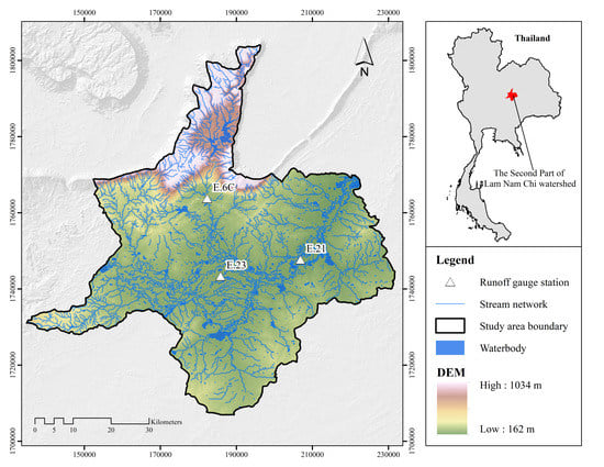
Figure 1. Terrain characteristics of the study area with runoff gauge stations.

3. Materials and Methods

The research methodology consisted of data collection and preparation and five significant components, which were (1) LULC classification, (2) LULC prediction, (3) surface runoff estimation, (4) optimization of LULC allocation for flood mitigation and mapping, and (5) economic and ecosystem service value evaluation and change (Figure 2). Details of each stage are separately described in the following sections.

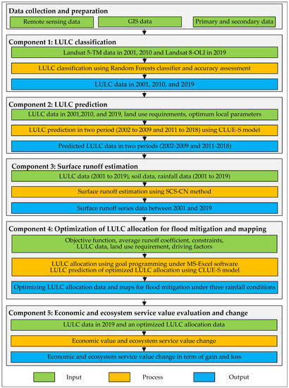
Figure 2. Workflow of the research methodology.

3.1. Data Collection and Preparation

The required input data for data analysis included GIS data, remote sensing data, and primary and secondary data, which were collected and prepared, as summarized in Table 1.

Table 1. List of data collection and preparation for data analysis in this study.

Data	Data Collection	Data Preparation	Source
Primary	Ground reference	-	-
Secondary	Runoff	-	RID
	Annual rainfall	Interpolation	TMD
	Socioeconomic data	Population density	DOPA
		Income per capita	NESDC
Remote Sensing	Landsat 5 TM: Path 128 Row 49, 6 January 2001 Landsat 5 TM: Path 129 Row 49, 14 February 2001 Landsat 5 TM: Path 128 Row 49, 16 February 2010 Landsat 5 TM: Path 129 Row 49, 23 February 2010 Landsat 8 OLI: Path 128 Row 49, 24 January 2019 Landsat 8 OLI: Path 129 Row 49, 31 January 2019	-	USGS
	Satellite image from Google Earth in 2010	-	Google
	Color orthophotograph	-	RTSD
GIS	Administrative boundary	-	DEQP
	Soil (soil series)	Recode	LDD
	Watershed boundary	-	RID
	Elevation	Extract from DEM	SRTM
	Slope	Extract from DEM	SRTM
	Road network	Buffering	MOT, DEQP
	Stream	Buffering	RTSD
	Urban area	Buffering	LULC data

Note: USGS, United States Geological Survey; RTSD, Royal Thai Survey Department; DEQP, Department of Environmental Quality Promotion; TMD, Thai Meteorological Department; RID, Royal Irrigation Department; LDD, Land Development Department; NESDC, Office of the National Economic and Social Development Council; SRTM, Shuttle Radar Topography Mission; MOT, Ministry of Transport; DOPA, Department of Provincial Administration.

3.2. LULC Classification

Landsat imageries in 2001, 2010, and 2019 were downloaded from the USGS website (www.earthexplore.usgs.gov, accessed on 22 November 2021) for LULC classification using the RF classifier of the EnMap-Box software. In practice, the training areas of each LULC type in a specific year were separately prepared to extract multiple decision trees for LULC classification. Spectral reflectance data (visible, NIR, and SWIR bands), additional spectral bands, and elevation were applied to classify the LULC types. The spectral bands that enhance particular features for LULC classification include the Normalized Difference Vegetation Index (NDVI) to represent vegetation features [29], the Modified Normalized Difference Wetness Index (MNDWI) to signify the moisture regime [30], and the Normalized Difference Built-up Index (NDBI) to indicate built-up areas [31]. Likewise, elevation is directly related to the spatial distribution of LULC type, e.g., paddy fields are generally situated in the floodplain, while forests are primarily located in mountainous areas.

In this study, the modified land use classification of the LDD consisted of (1) urban and built-up areas, (2) paddy fields, (3) sugarcane, (4) cassava, (5) other field crops, (6) para rubber, (7) perennial trees and orchards, (8) forest land, (9) waterbodies, (10) rangeland, (11) marshes and swamps, and (12) unused land.

After classification, the LULC maps in 2001, 2010, and 2019 were assessed for thematic accuracy (overall accuracy and Kappa hat coefficient) based on the reference data from color orthophotograph in 2000–2001, very high spatial resolution imageries from Google Earth in 2010, and field surveys in 2020, respectively. This study estimated the number of sample sizes for thematic accuracy assessment based on multinomial distribution with a stratified random sampling scheme, as suggested by [32].

3.3. LULC Prediction

The CLUE-S model was selected to predict LULC data in two periods, 2002–2009 and 2011–2018, for filling the gap of LULC data between three classified LULC data in 2001, 2010, and 2019. As a result, time-series LULC data between 2001 and 2019 will be available for annual surface runoff estimation in this study.

3.3.1. Optimal Local Driving Factors on Land Use Change Identification for LULC Prediction

The land use change model CLUE-S was selected to predict the LULC data in two periods, 2002–2009 and 2011–2018, for data analysis. The local driving factors on land use change for LULC prediction were identified by comparing the predicted LULC map in 2019 with the classified LULC map in 2019. The basic parameters of the CLUE-S model, which include (1) elasticity value, (2) LULC conversion matrix, and (3) land requirement of each LULC type in 2019, were firstly extracted based on the final LULC map in 2001 and 2010 using the Markov Chain model. At the same time, the selected three driving factor categories on LULC change, including physical, socioeconomic, and proximity data, which were reviewed from the previous studies of many researchers [33,34,35,36,37,38,39,40,41,42,43,44,45], were examined multicollinearity, and significant driving factors for LULC identified by allocating using binomial logistic regression analysis, as follows:

$$\mathrm{Log}\left(\frac{{\mathrm{P}}_{\mathrm{i}}}{1-{\mathrm{P}}_{\mathrm{i}}}\right)={\mathsf{\beta }}_0+{\mathsf{\beta }}_1{\mathrm{X}}_{1,\mathrm{i}}+{\mathsf{\beta }}_2{\mathrm{X}}_{2,\mathrm{i}}\dots \dots +{\mathsf{\beta }}_{\mathrm{n}}{\mathrm{X}}_{\mathrm{n},\mathrm{i}}$$

(1)

where P_i is the probability of a grid cell for the considered land use type on location i, and the Xs are the location factors. The coefficients (β) were estimated through logistic regression using the actual land use pattern as the dependent variable [46].

After this, the predicted LULC map in 2019 was compared to the classified map in 2019 using a wall-to-wall thematic accuracy assessment with overall accuracy and Kappa hat coefficient. If the overall accuracy and Kappa hat coefficient were equal to or more than 80%, then the derived significant driving factors by binomial logistic regression analysis were chosen as the optimal local driving factors on land use change for LULC prediction using the CLUE-S model.

3.3.2. LULC Prediction of Two Periods: 2002–2009 and 2011–2018

The optimal local driving factors on land use change for LULC prediction, namely, elasticity value, LULC conversion matrix, and land requirement of each LULC type in two time periods (2002–2009 and 2011–2018), which were extracted using the Markov Chain model based on the corresponding LULC data in 2001, 2010, and 2019, were applied to predict the LULC data in the two periods using the CLUE-S model.

3.4. Surface Runoff Estimation

This study estimated the time series surface runoff between 2001 and 2019 based on the classified and predicted LULC data, soil series, and rainfall data using the SCS-CN method with suitable AMC via ESRI ArcGIS software.

In practice, the required input data included LULC, soil series, rainfall, and hydrologic soil group data, prepared and operated for surface runoff estimation using the SCS-CN method in raster format with a cell size of 30 m in a raster-based GIS environment. The surface runoff depth in each cell was semi-automatically generated based on runoff curve numbers (CNs) according to hydrologic soil group–land cover complex using the Model Builder of ArcGIS, as shown in Figure 3.

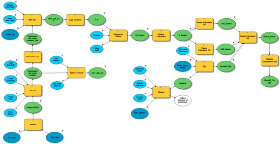
Figure 3. Schematic diagram of Model Builder for surface runoff estimation.

The soil series data, which were applied to classify soil texture classes based on the percentage of sand, silt, and clay of each soil series unit, are displayed in Figure 4a. Meanwhile, the hydrologic soil group (HSG), which presents potential runoff in the study area according to soil texture classes, is shown in Figure 4b.

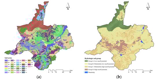
Figure 4. Spatial distribution of (a) soil series and (b) hydrologic soil group.

In this study, two significant steps implemented under this component include (1) suitable AMC for surface runoff estimation using the SCS-CN method and (2) surface runoff estimation between 2011 and 2019.

3.4.1. Suitable AMC for Surface Runoff Estimation Using the SCS-CN Method

The suitable AMC condition for surface runoff estimation using the SCS-CN method was examined based on the classified and predicted LULC data between 2001 and 2010 with three different CN values of three different AMCs, as suggested by [47] using the following equations:

$${\mathrm{CN}}_{\mathrm{I}}=\frac{4{.2\mathrm{CN}}_{\mathrm{II}}}{10-0{.058\mathrm{CN}}_{\mathrm{II}}}$$

(2)

$${\mathrm{CN}}_{\mathrm{III}}=\frac{{23\mathrm{CN}}_{\mathrm{II}}}{10+0{.13\mathrm{CN}}_{\mathrm{II}}}$$

(3)

where ${\mathrm{CN}}_{\mathrm{I}}$ is the runoff curve number value of each LULC type of AMC-I, ${\mathrm{CN}}_{\mathrm{II}}$ is the runoff curve number value of each LULC type of AMC-II, and ${\mathrm{CN}}_{\mathrm{III}}$ is the runoff curve number value of each LULC type of AMC-III (Table 2).

Table 2. Runoff curve number under AMC-I, -II, and -III.

LULC Types	CN Value of AMC-I				CN Value of AMC-II				CN Value of AMC-III
	A	B	C	D	A	B	C	D	A	B	C	D
Urban and built-up area	77.26	82.85	86.81	88.86	89	92	94	95	94.9	96.36	97.3	97.76
Cassava and other field crops	51.92	64.16	75.49	80.94	72	81	88	91	85.54	90.75	94.4	95.88
Sugarcane	28.75	48.32	61.24	68.8	49	69	79	84	68.85	83.66	89.64	92.35
Paddy fields	43.82	57.08	68.8	75.49	65	76	84	88	81.03	87.93	92.35	94.4
Rangeland	28.75	48.32	61.24	68.8	49	69	79	84	68.85	83.66	89.64	92.35
Para rubber and perennial trees and orchards	24.06	43.82	57.08	65.68	43	65	76	82	63.44	81.03	87.93	91.29
Forest land	15.25	33.92	49.49	58.44	30	55	70	77	49.64	73.76	84.29	88.51
Waterbodies and marshes and swamps	95.37	95.37	95.37	95.37	98	98	98	98	99.12	99.12	99.12	99.12
Unused land	58.44	72.07	80.94	86.81	77	86	91	94	88.51	93.39	95.88	97.3

In practice, the three runoff curve numbers of the hydrologic soil group of each LULC type were separately applied to estimate the potential maximum storage under three different AMCs using Equation (4).

$$\mathrm{S}=25.4\frac{1000}{\mathrm{CN}}-10$$

(4)

where $\mathrm{CN}$ is the runoff curve number of the hydrologic soil group (HSG)–land cover complex.

The calculated potential maximum storage was further applied to estimate the surface runoff depth of the three different AMCs [48,49], as follows:

$$\mathrm{Q}=\frac{{\left(\mathrm{P}-0.2\mathrm{S}\right)}^2}{\left(\mathrm{P}+0.8\mathrm{S}\right)}$$

(5)

where $\mathrm{Q}$ is the surface runoff depth (mm), $\mathrm{P}$ is the annual rainfall (mm), and $\mathrm{S}$ is the potential maximum storage.

Then, the estimated surface runoff depth of the three different AMCs from 2001 to 2010 was converted into surface runoff volume using Equation (6).

$$\mathrm{Surface}\mathrm{runoff}\mathrm{volume}=\frac{\mathrm{Surface}\mathrm{runoff}\mathrm{depth}}{1000} \times \mathrm{cell} \mathrm{size}$$

(6)

Later, they were used to identify the suitable AMC using model performance scale, including Nash and Sutcliffe’s coefficient of efficiency (NSE), the coefficient of determination (R²), and the percent of bias (PBIAS) (Equations (7)–(9)), as suggested by [50] (Table 3).

$$\mathrm{NSE}=1-\left[\frac{{{\displaystyle \sum }}_{\mathrm{i}}^{\mathrm{n}}{\left({\mathrm{Q}}_{\mathrm{simi}}-{\mathrm{Q}}_{\mathrm{obsi}}\right)}^2}{{{\displaystyle \sum }}_{\mathrm{i}}^{\mathrm{n}}{\left({\mathrm{Q}}_{\mathrm{obsi}}-{\mathrm{Q}}_{\mathrm{avg}}\right)}^2}\right]$$

(7)

where $\mathrm{n}$ is the number of years, ${\mathrm{Q}}_{\mathrm{simi}}$ is the simulated surface runoff, ${\mathrm{Q}}_{\mathrm{obsi}}$ is the observed surface runoff, and ${\mathrm{Q}}_{\mathrm{avg}}$ is the average observed surface runoff over the simulation period. The values for E can vary from –∞ to 1, with 1 indicating a perfect fit.

$${\mathrm{R}}^2={\left\{\frac{{{\displaystyle \sum }}_{\mathrm{i}=1}^{\mathrm{n}}\left({\mathrm{Q}}_{\mathrm{obsi}}-{\mathrm{Q}}_{\mathrm{obsavg}}\right)\left({\mathrm{Q}}_{\mathrm{simi}}-{\mathrm{Q}}_{\mathrm{simavg}}\right)}{{\left[{{\displaystyle \sum }}_{\mathrm{i}=1}^{\mathrm{n}}{\left({\mathrm{Q}}_{\mathrm{obsi}}-{\mathrm{Q}}_{\mathrm{obsav}}{}_{\mathrm{g}}\right)}^2{{\displaystyle \sum }}_{\mathrm{i}=1}^{\mathrm{n}}{\left({\mathrm{Q}}_{\mathrm{simi}}-{\mathrm{Q}}_{\mathrm{simavg}}\right)}^2\right]}^{0.5}}\right\}}^2$$

(8)

where ${\mathrm{Q}}_{\mathrm{obsi}}$ is the observed surface runoff in year $\mathrm{i}$, ${\mathrm{Q}}_{\mathrm{simi}}$ is the simulated surface runoff in year $\mathrm{i}$, ${\mathrm{Q}}_{\mathrm{obsavg}}$ is the average of the observed surface runoff over the calibration or validation period, ${\mathrm{Q}}_{\mathrm{simavg}}$ is the average of the simulated surface runoff over the validation period, $\mathrm{i}$ is the year, and $\mathrm{n}$ is the total count of data pairs.

$$\mathrm{PBIAS}=\left[\frac{{{\displaystyle \sum }}_{\mathrm{i}=1}^{\mathrm{n}}\left({\mathrm{Y}}_{\mathrm{i}}^{\mathrm{obs}}-{\mathrm{Y}}_{\mathrm{i}}^{\mathrm{sim}}\right)\text{×}\left(100\right)}{{{\displaystyle \sum }}_{\mathrm{i}=1}^{\mathrm{n}}{\mathrm{Y}}_{\mathrm{i}}^{\mathrm{obs}}}\right]$$

(9)

where ${\mathrm{Y}}_{\mathrm{i}}^{\mathrm{obs}}$ is the observed surface runoff in time step $\mathrm{i}$, and ${\mathrm{Y}}_{\mathrm{i}}^{\mathrm{sim}}$ is the simulated surface runoff in time step $\mathrm{i}$.

Table 3. Model performance scale.

Statistics Measurement	Performance Ratings
	Unsatisfactory	Satisfactory	Good	Very Good
NSE	<0.5	0.5–0.65	0.65–0.75	0.75–1
R2	<0.5	0.5–0.6	0.6–0.7	0.7–1
PBIAS	>25	15–25	10–15	<10

In this study, the observed runoff data between 2001 and 2010 from the hydrological station at E.21, E.23, and E.6C of the RID were used to calculate an average NSE, R², and PBIAS for suitable AMC identification (see the location of the station in Figure 1).

3.4.2. Surface Runoff Estimation between 2011 and 2019

The runoff curve number of the suitable AMC was applied to estimate the surface runoff between 2011 and 2019 based on the classified and predicted LULC data in the same period. The estimated surface runoff data between 2011 and 2019 were further examined for model validation based on the observed runoff data in the same period from the same gauges of the RID using NSE, R², and PBIAS.

The time series surface runoff estimation (between 2001 and 2019) from two steps will be further applied to extract the average runoff coefficient of each LULC type of three rainfall conditions for optimizing LULC allocation for flood mitigation in the next component.

3.5. Optimization of LULC Allocation for Flood Mitigation and Mapping

Goal programming was first applied to optimize LULC allocation for flood mitigation under dry, normal, and wet years. Then, the suitable LULC allocation data of dry, normal, and wet years were mapped using the CLUE-S model.

3.5.1. SPI Calculation for the Rainfall Condition Identification

Annual rainfall data between 1987 and 2019 were first used to calculate the 12-month SPI values. Then, they were reclassified into three rainfall conditions according to the SPI drought classification of [51] as follows:

• If any year had a 12-month SPI value less than or equal to –0.50, the annual rainfall was categorized as a dry year;
• If any year had a 12-month SPI value between –0.49 and 0.49, the annual rainfall was categorized as a normal year;
• If any year had a 12-month SPI value more than or equal to 0.50, the annual rainfall was categorized as a wet year.

After that, the average surface runoff coefficient for each LULC type of three rainfall conditions (dry, normal, and wet years) was extracted from the time series surface runoff and LULC data using zonal statistical analysis for optimization of LULC allocation to minimize surface runoff for flood mitigation.

3.5.2. Optimization of LULC Allocation to Minimize Surface Runoff for Flood Mitigation

This study assigned the constraint sets for optimizing LULC allocation in 2029, 2039, and 2049 using the Markov Chain model based on the historical LULC development between 2010 and 2019. The changing area of each LULC type was considered according to the derived transitional change area from the Markov Chain model. Then, the derived average runoff coefficient and constraints of the objective function were applied to optimize LULC allocation to minimize surface runoff for flood mitigation under dry, normal, and wet years using goal programming with “What’s Best!” as an extension program in an MS Excel environment.

The goal programming model, working as the surface runoff minimization function, can be expressed as the following equations:

Minimize surface runoff:

$$\mathrm{Min}\left(\mathrm{z}\right)={\displaystyle \sum }_{\mathrm{i}=1}^{\mathrm{n}}{\mathrm{C}}_{\mathrm{i}}{\mathrm{X}}_{\mathrm{i}}$$

(10)

Subject to constraints:

$${\displaystyle \sum }_{\mathrm{i}=1}^{\mathrm{n}}{\mathrm{X}}_{\mathrm{i}}=\mathrm{A}$$

(11)

$${\displaystyle \sum }_{\mathrm{i}=1}^{\mathrm{n}}{\mathrm{X}}_{\mathrm{i}}\ge \mathrm{A}$$

(12)

$${\displaystyle \sum }_{\mathrm{i}=1}^{\mathrm{n}}{\mathrm{X}}_{\mathrm{i}}\le \mathrm{A}$$

(13)

$${\mathrm{X}}_{\mathrm{i}}\ge 0$$

(14)

where $\mathrm{Z}$ is the total annual surface runoff of the study area (m³/year), ${\mathrm{C}}_{\mathrm{i}}$ is the average surface runoff coefficient in each land use type (m³/km²/year), ${\mathrm{X}}_{\mathrm{i}}$ is the area of land use class $\mathrm{i}$ (km²), $\mathrm{n}$ is the number of land use classes, and $\mathrm{A}$ is the total area of land use classes (km²).

Finally, the suitable LULC allocation to minimize surface runoff for flood mitigation under dry, normal, and wet years was separately identified based on surface runoff reduction compared to the actual data in 2019.

3.5.3. Mapping of Suitable LULC Allocation for Flood Mitigation

The suitable LULC allocation to minimize surface runoff for flood mitigation under dry, normal, and wet years was separately mapped using the CLUE-S model. The required input data for LULC mapping included LULC data in 2019, local driving factors on land use change, elasticity value, LULC conversion matrix, and suitable LULC allocation data of three rainfall conditions as the land requirement.

3.6. Economic and Ecosystem Service Value Evaluation and Change

Economic and ecosystem service value evaluation and change were separately evaluated using the present value (PV) model and the simple benefit transfer method based on LULC data in 2019 and suitable LULC allocation data to minimize surface runoff for flood mitigation under dry, normal, and wet years in terms of gain and loss.

3.6.1. Economic Value Evaluation and Change

For economic value evaluation, the LULC data in 2019 and the suitable LULC allocation data to minimize surface runoff under dry, normal, and wet years were first calculated in terms of economic values using Equation (15), as suggested by [52]. Then, the future economic value changes between the LULC data in 2019 and the suitable LULC allocation data to minimize surface runoff under dry, normal, and wet years were compared using the image algebra change detection algorithm for gain and loss.

$$\mathrm{PV}=\mathrm{FV}\cdot {\left[\frac{100}{100+\mathrm{IR}}\right]}^{\mathrm{Y}}$$

(15)

where $\mathrm{PV}$ is the present value, $\mathrm{FV}$ is the future value, $\mathrm{IR}$ is the interest rate in percent, and $\mathrm{Y}$ is the number of years from the present, counting from zero.

3.6.2. Ecosystem Service Value Evaluation and Change

In general, ecosystem services represent a dynamic field in current scientific research, linking ecological, economic, and social aspects, demanding practical applications and methodologies at different spatial scales, and maintaining environmental management and decision-making processes [53,54,55].

This study applied a simple benefit transfer method [53] to evaluate the ecosystem service values of LULC data in 2019 and suitable LULC allocation data to minimize surface runoff under dry, normal, and wet years using Equation (16) with the coefficient value for different LULC types (Table 4). Then, the ecosystem service value change between the LULC data in 2019 and the suitable LULC allocation data to minimize surface runoff under dry, normal, and wet years was compared using the image algebra change detection algorithm for gain and loss.

$$\mathrm{ESV}={{\displaystyle \sum }}^{ }\left({\mathrm{A}}_{\mathrm{k}}{ \times \mathrm{VC}}_{\mathrm{k}}\right)$$

(16)

where $\mathrm{ESV}$ denotes the total value of the ecosystem service, while ${\mathrm{A}}_{\mathrm{k}}$ and ${\mathrm{VC}}_{\mathrm{k}}$ represent the area and value coefficient for proxy LULC type $“\mathrm{k},”$ respectively.

Table 4. LULC type and coefficient value for ESV evaluation.

No.	LULC Classification for RF	LULC Classification for ESV 1	Coefficient Values (USD/ha/year) 1
1	Urban and built-up areas	Construction land	12.7
2	Paddy fields	Cultivated land	1032.3
3	Field crops	Cultivated land	1032.3
4	Para rubber	Forest land	1949.0
5	Perennial trees and orchards	Forest land	1949.0
6	Forest land	Forest land	1949.0
7	Waterbodies	Waterbodies	6873.7
8	Rangeland	Rangeland	808.6
9	Wetland	Wetland	9368.7
10	Miscellaneous land	Unused land	96.3

¹ Modified from [56].

Finally, the future economic and ecosystem service values and their changes in suitable LULC allocation for flood mitigation by each rainfall condition (dry, normal, and wet years) were compared to justify the most suitable LULC allocation for flood mitigation among three rainfall conditions.

4. Results and Discussion

4.1. Land Use and Land Cover Classification and Change Detection

The results of the LULC classification in 2001, 2010, and 2019 using the random forests (RF) classifier based on Landsat imageries and supplementary data, including NDVI, MNDWI, NDBI, and DEM, are reported in Table 5 and displayed in Figure 5.

Table 5. Area and percentage of LULC data in 2001, 2010, and 2019.

No.	LULC Type	LULC 2001		LULC 2010		LULC 2019
		Area (km2)	Percentage	Area (km2)	Percentage	Area (km2)	Percentage
1	Urban and built-up areas	46.17	1.22	53.21	1.4	65.84	1.74
2	Paddy fields	2344.39	61.79	2070.71	54.58	2012.16	53.03
3	Sugarcane	61.25	1.61	153.52	4.05	306.85	8.09
4	Cassava	532.95	14.05	629.33	16.59	489.91	12.91
5	Other field crops	2.09	0.06	5.19	0.14	6.19	0.16
6	Para rubber	16.56	0.44	30.05	0.79	97.03	2.56
7	Perennial trees and orchards	55.76	1.47	50.21	1.32	88.95	2.34
8	Forest land	632	16.66	604.7	15.94	481.3	12.68
9	Waterbodies	36.81	0.97	57.46	1.51	53.3	1.4
10	Rangeland	26.03	0.69	72.11	1.9	71.65	1.89
11	Marshes and swamps	11.64	0.31	33.4	0.88	27.73	0.73
12	Unused land	28.57	0.75	34.33	0.9	93.32	2.46
Total		3794.22	100.00	3794.22	100.00	3794.22	100.00

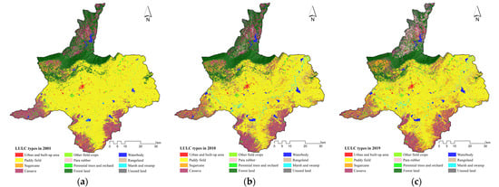
Figure 5. Spatial distribution of the LULC classification in: (a) 2001, (b) 2010, and (c) 2019.

The results reveal that in 2001, the top three most dominant LULC types were paddy fields (61.79%), forest land (16.66%), and cassava (14.05%). On the contrary, the top three least dominant LULC types were other field crops (0.06%), marshes and swamps (0.30%), and para rubber (0.44%), which are randomly distributed in the study area. Meanwhile, the top three most dominant in 2019 were paddy fields (54.58%), cassava (16.59%), and forest land (15.94%). Conversely, the top three least dominant LULC types in 2001 were other field crops (0.14%), marshes and swamps (0.79%), and para rubber (0.88%). Recently, the top three most dominant LULC types in 2019 were paddy fields (53.03%), cassava (12.91%), and forest land (12.68%). In contrast, the top three least dominant LULC types were other field crops (0.16%), marshes and swamps (0.73%), and waterbodies (1.40%). The temporal change in LULC type coverage in 2001, 2010, and 2019 is presented in Figure 6.

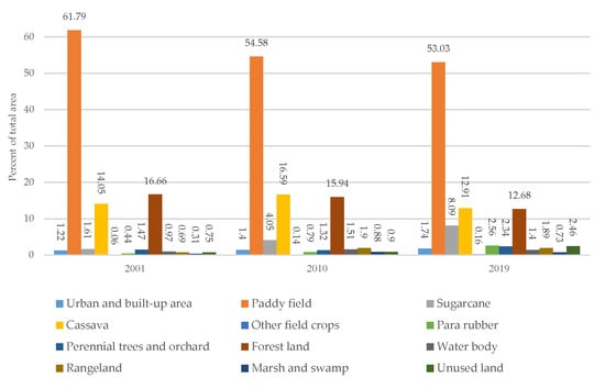
Figure 6. Multitemporal change of LULC type coverage in 2001, 2010, and 2019.

Furthermore, a simple comparison of the LULC type coverage with the changing area, annual change rate, and percentage of in two short periods (2001–2010 and 2010–2019) and in the long period (2001–2019) are reported in Table 6, Table 7 and Table 8. The annual change rate of the short- and long-term periods plays a significant role in land requirement estimation for LULC prediction using the CLUE-S model.

Table 6. Simple LULC change detection between 2001 and 2010.

LULC	LULC Type (Area, km2)
	UR	PA	SU	CA	PC	PR	PO	FO	WA	RA	MA	UL
In 2001	46.17	2344.39	61.25	532.95	2.09	16.56	55.76	632.00	36.81	26.03	11.64	28.57
In 2010	53.21	2070.71	153.52	629.33	5.19	30.05	50.21	604.70	57.46	72.11	33.40	34.33
Change area	7.04	–273.68	92.27	96.38	3.11	13.49	–5.54	–27.30	20.65	46.08	21.76	5.76
Annual change rate	0.78	–30.41	10.25	10.71	0.35	1.50	–0.62	–3.03	2.29	5.12	2.42	0.64
Percentage of change	0.19	–7.21	2.43	2.54	0.08	0.36	–0.15	–0.72	0.54	1.21	0.57	0.15

Table 7. Simple LULC change detection between 2010 and 2019.

LULC	LULC Type (Area, km2)
	UR	PA	SU	CA	PC	PR	PO	FO	WA	RA	MA	UL
In 2010	53.21	2070.71	153.52	629.33	5.19	30.05	50.21	604.70	57.46	72.11	33.40	34.33
In 2019	65.84	2012.16	306.85	489.91	6.19	97.03	88.95	481.30	53.30	71.65	27.73	93.32
Change area	12.63	–58.55	153.33	–139.41	1.00	66.99	38.73	–123.41	–4.16	–0.47	–5.67	58.99
Annual change rate	1.40	–6.51	17.04	–15.49	0.11	7.44	4.30	–13.71	–0.46	–0.05	–0.63	6.55
Percentage of change	0.33	–1.54	4.04	–3.67	0.03	1.77	1.02	–3.25	–0.11	–0.01	–0.15	1.55

Table 8. Simple LULC change detection between 2001 and 2019.

LULC	LULC Type (Area, km2)
	UR	PA	SU	CA	PC	PR	PO	FO	WA	RA	MA	UL
In 2001	46.17	2344.39	61.25	532.95	2.09	16.56	55.76	632	36.81	26.03	11.64	28.57
In 2019	65.84	2012.16	306.85	489.91	6.19	97.03	88.95	481.3	53.3	71.65	27.73	93.32
Change area	19.67	–332.23	245.6	–43.04	4.1	80.47	33.19	–150.7	16.49	45.62	16.09	64.75
Annual change rate	1.09	–18.46	13.64	–2.39	0.23	4.47	1.84	–8.37	0.92	2.53	0.89	3.60
Percentage of change	0.52	–8.76	6.47	–1.13	0.11	2.12	0.87	–3.97	0.43	1.20	0.42	1.71

Moreover, by considering the performance of the RF classifier for LULC classification, the overall accuracy and Kappa hat coefficient of the classified LULC maps in 2001 were 89.88% and 84.88%, in 2010 were 90.71% and 87.03%, and in 2019 were 91.37% and 88.26%. The overall accuracy of more than 85% of the three maps provides acceptable results, as suggested by [57]. Likewise, the Kappa hat coefficient of the three maps was more than 80%, representing strong agreement or accuracy between the classified map and the ground reference information [58]. The derived overall accuracy and Kappa hat coefficient values of the classified LULC maps are comparable to those of other researchers who classified LULC maps based on Landsat data with the RF classifier [44,59,60,61,62,63,64,65]

4.2. Driving Factor Identification for LULC Change

The results of the binary logistics regression analysis for identifying LULC type location preference after the multicollinearity test are reported in Table 9. The most common vital driving factor for all LULC type changes was elevation. Meanwhile, the most important driving factors for field crops (sugarcane, cassava, and other field crops) included elevation, slope, and annual rainfall. The specific driving factors for each LULC type preference from binary logistics regression are further applied to allocate LULC type for predicting LULC change under the CLUE-S model.

Table 9. Multiple linear equations of each LULC type location preference and area under the curve value from logistic regression analysis.

Driving Factors	LULC Type
	UR	PD	SU	CA	FC	PR	OP	FO	WA	RA	MA	UL
Constant	0.0930	10.8831	94.6560	–38.4766	207.9784	24.1870	–38.4831	87.3484	–4.6862	–80.0118	5.0436	–8.6344
X1	n. s.	–0.0947	–0.0001	0.0042	0.0101	0.0083	n. s.	0.0032	0.0068	–0.0043	–0.0467	0.0093
X2	n. s.	n. s.	–0.1943	–0.1030	–0.2144	–0.0730	–0.1314	0.1886	–0.6715	n. s.	n. s.	–0.0290
X3	n. s.	0.0130	–0.1264	0.0477	–0.2850	–0.0398	0.0454	–0.1167	n. s.	0.0991	n. s.	n. s.
X4	n. s.	n. s.	n. s.	n. s.	n. s.	n. s.	n. s.	n. s.	n. s.	n. s.	n. s.	n. s.
X5	0.0008	–0.0018	–0.0117	–0.0148	n. s.	–0.0186	–0.0043	–0.0113	n. s.	–0.0060	–0.0059	n. s.
X6	–0.0064	n. s.	n. s.	n. s.	n. s.	n. s.	n. s.	n. s.	0.0014	n. s.	n. s.	n. s.
X7	n. s.	n. s.	n. s.	0.0010	n. s.	–0.0014	n. s.	n. s.	–0.0037	n. s.	–0.0053	n. s.
X8	–0.0182	n. s.	n. s.	n. s.	n. s.	n. s.	n. s.	n. s.	n. s.	n. s.	n. s.	n. s.
AUC	0.9824	0.9763	0.7677	0.7942	0.9355	0.9440	0.6186	0.9289	0.8318	0.7445	0.8628	0.8693

Note: Elevation (X₁), slope (X₂), annual rainfall (X₃), average income per capita at the sub-district level (X₄), population density at the sub-district level (X₅), distance to road network (X₆), distance to stream (X₇), and distance to the existing urban area (X₈).

Moreover, the derived area under the curve (AUC) values for each LULC type allocation varied from 0.6185 to 0.9824. This finding suggests a fair-to-excellent fit between the predicted and real LULC transition [66,67,68].

4.3. Local Parameter for LULC Prediction Using the CLUE-S Model

After a wall-to-wall accuracy assessment, by comparison, for the predicted LULC in 2019 with the classified LULC in 2019, the overall accuracy was 86.95%, and the Kappa hat coefficient was 80.72%. Thus, the significant driving factors by binomial logistic regression analysis were chosen as the optimal local driving factors on land use change for LULC prediction using the CLUE-S model in this study (see Table 9).

In the meantime, the optimal conversion matrix for each LULC type possibly changed between 2010 and 2019 (Table 10) and the land use type resistance (elasticity) values based on the transition probability matrix of LULC changed between 2010 and 2019 from the Markov Chain model (Table 11), identified as a local parameter for LULC prediction. Thus, the elasticity value of the urban and built-up areas, paddy fields, sugarcane, cassava, other field crops, para rubber, perennial trees and orchards, forest land, waterbodies, rangeland, marshes and swamps, and unused land were 1.00, 0.93, 0.93, 0.65, 0.99, 0.80, 0.99, 0.80, 0.91, 0.89, 0.39, and 0.96, respectively.

Table 10. Conversion matrix of possible changes between 2010 and 2019.

	LULC Types	LULC Type Possible Change in 2019
		UR	PA	SU	CA	FC	PR	PO	FO	WA	RA	MA	UL
LULC in 2010	Urban and built-up areas (UR)	1	0	0	0	0	0	0	0	0	0	0	0
	Paddy fields (PA)	0	1	1	1	0	0	1	0	0	1	1	0
	Sugarcane (SU)	1	1	1	1	0	0	1	0	0	0	0	0
	Cassava (CA)	1	1	1	1	0	1	1	0	0	1	0	1
	Other field crops (FC)	0	0	1	1	1	0	0	0	0	0	0	0
	Para rubber (PR)	0	0	0	1	1	1	0	0	0	0	0	1
	Perennial trees and orchards (PO)	0	0	1	0	0	0	1	0	0	0	0	0
	Forest land (FO)	1	0	0	0	0	1	1	1	0	1	0	1
	Waterbodies (WA)	1	0	1	0	0	0	0	0	1	0	1	0
	Rangeland (RA)	0	1	0	0	0	0	1	0	0	1	0	0
	Marshes and swamps (MA)	1	1	1	1	0	0	1	0	0	0	1	0
	Unused land (UL)	1	1	0	0	0	0	0	0	0	0	0	1

Table 11. Elasticity of LULC change for LULC prediction between 2010 and 2019.

	LULC Types	LULC Type Possible Change in 2019
		UR	PA	SU	CA	FC	PR	PO	FO	WA	RA	MA	UL
LULC in 2010	Urban and built-up areas (UR)	1.00	-	-	-	-	-	-	-	-	-	-	-
	Paddy fields (PA)	-	0.93	0.03	0.02	-	-	0.01	-	-	-	0.01	-
	Sugarcane (SU)	0.01	0.01	0.93	0.05	-	-	0.01	-	-	-	-	-
	Cassava (CA)	0.01	0.06	0.16	0.65	-	0.07	0.01	-	-	-	-	0.04
	Other field crops (FC)	-	-	-	-	0.99	-	0.01	-	-	-	-	-
	Para rubber (PR)	-	-	-	0.11	0.01	0.80	0.03	-	-	-	-	0.05
	Perennial trees and orchards (PO)	-	-	0.01	0.01	-	-	0.99	-	-	-	-	-
	Forest land (FO)	-	0.02	-	0.05	-	0.05	0.01	0.80	-	-	-	0.06
	Waterbodies (WA)	-	0.04	0.02	0.01	-	-	-	-	0.91	-	0.01	-
	Rangeland (RA)	-	0.08	-	0.02	-	-	0.01	-	-	0.89	-	-
	Marshes and swamps (MA)	0.01	0.55	0.03	-	-	-	0.02	-	-	-	0.39	-
	Unused land (UL)	0.01	0.03	-	-	-	-	-	-	-	-	-	0.96

4.4. LULC Prediction between 2002 and 2009

LULC prediction data between 2002 and 2009, which were simultaneously allocated based on the conversion matrix of LULC change (Table 10), elasticity value (Table 11), annual land demand (Table 12), and driving factors on LULC change for specific LULC type location preference (Table 9), are reported in Table 13 and displayed in Figure 7.

Table 12. Annual land requirement of each LULC type between 2001 and 2010.

Year	LULC Type (Area, km2)												Total
	UR	PA	SU	CA	FC	PR	PO	FO	WA	RA	MA	UL
2001	46.17	2344.39	61.25	532.95	2.09	16.56	55.76	632.00	36.81	26.03	11.64	28.57	3794.22
2002	46.95	2314.01	71.53	543.60	2.45	18.03	55.15	628.98	39.12	31.16	14.03	29.19	3794.22
2003	47.71	2283.59	81.77	554.34	2.79	19.54	54.54	625.95	41.40	36.28	16.46	29.84	3794.22
2004	48.50	2253.18	91.96	565.05	3.13	21.09	53.90	622.90	43.70	41.38	18.94	30.47	3794.22
2005	49.30	2222.70	102.27	575.78	3.50	22.54	53.27	619.88	46.00	46.51	21.30	31.16	3794.22
2006	50.05	2192.30	112.51	586.50	3.83	24.10	52.66	616.83	48.28	51.63	23.78	31.74	3794.22
2007	50.82	2161.94	122.76	597.16	4.17	25.57	52.07	613.81	50.57	56.77	26.17	32.40	3794.22
2008	51.61	2131.48	133.03	607.87	4.51	27.08	51.47	610.77	52.86	61.90	28.60	33.03	3794.22
2009	52.41	2101.12	143.27	618.63	4.87	28.53	50.84	607.74	55.16	66.99	30.97	33.69	3794.22
2010	53.21	2070.70	153.51	629.33	5.19	30.05	50.21	604.70	57.46	72.11	33.40	34.33	3794.22
Annual rate	0.79	–30.42	10.24	10.71	0.33	1.52	–0.63	–3.03	2.29	5.12	2.44	0.64

Table 13. Area of predicted LULC type between 2002 and 2009.

LULC Types	Area of Predicted LULC Type (km2)
	2002	2003	2004	2005	2006	2007	2008	2009
Urban and built-up areas (UR)	46.95	47.71	48.5	49.3	50.05	50.82	51.61	52.41
Paddy fields (PD)	2314.01	2283.59	2253.18	2222.70	2192.30	2161.94	2131.48	2101.12
Sugarcane (SU)	71.53	81.77	91.96	102.27	112.51	122.76	133.03	143.27
Cassava (CA)	543.6	554.34	565.05	575.78	586.5	597.16	607.87	618.63
Other field crops (FC)	2.45	2.79	3.13	3.5	3.83	4.17	4.51	4.87
Para rubber (PR)	18.03	19.54	21.09	22.54	24.1	25.57	27.08	28.53
Perennial trees and orchards (PO)	55.15	54.54	53.9	53.27	52.66	52.07	51.47	50.84
Forest land (FO)	628.98	625.95	622.9	619.88	616.83	613.81	610.77	607.74
Waterbodies (WA)	39.12	41.4	43.7	46	48.28	50.57	52.86	55.16
Rangeland (RA)	31.16	36.28	41.38	46.51	51.63	56.77	61.9	66.99
Marshes and swamps (MA)	14.03	16.46	18.94	21.3	23.78	26.17	28.6	30.97
Unused land (UL)	29.19	29.84	30.47	31.16	31.74	32.4	33.03	33.69
Total	3794.22	3794.22	3794.22	3794.22	3794.22	3794.22	3794.22	3794.22

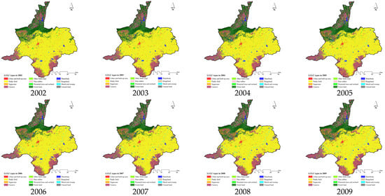
Figure 7. Spatial distribution of predicted LULC data between 2002 and 2009.

As a result, the LULC prediction between 2002 and 2009 was dictated by the historical LULC development between 2001 and 2010. The results indicate that the most increasing LULC types were cassava and sugarcane, with an increasing annual change rate of 10.71 and 10.24 km² per year, while the paddy field was the most decreasing LULC type with a decreasing annual change rate of 30.42 km² per year.

4.5. LULC Prediction between 2011 and 2018

The derived optimum local parameter of the CLUE-S model with annual land demand between 2010 and 2019 based on the annual change rate of the Markov Chain model (Table 14) was simultaneously combined with driving factors for LULC change for a specific LULC type location preference (Table 9) to predict LULC data, as shown by the results in Table 15 and Figure 8.

Table 14. Annual land requirement of each LULC type between 2010 and 2019.

Year	LULC Type (Area, km2)												Total
	UR	PA	SU	CA	FC	PR	PO	FO	WA	RA	MA	UL
2010	53.21	2070.71	153.52	629.33	5.19	30.05	50.21	604.70	57.46	72.11	33.40	34.33	3794.22
2011	54.58	2064.15	170.56	613.86	5.32	37.51	54.49	591.02	57.00	72.09	32.75	40.88	3794.22
2012	55.99	2057.68	187.61	598.35	5.43	44.93	58.80	577.30	56.54	72.03	32.13	47.42	3794.22
2013	57.46	2051.17	204.62	582.86	5.53	52.39	63.17	563.53	56.06	71.98	31.48	53.98	3794.22
2014	58.81	2044.70	221.65	567.39	5.65	59.83	67.42	549.87	55.61	71.85	30.90	60.55	3794.22
2015	60.27	2038.20	238.68	551.89	5.74	67.26	71.78	536.14	55.15	71.81	30.21	67.07	3794.22
2016	61.65	2031.64	255.75	536.39	5.87	74.71	76.06	522.43	54.70	71.81	29.59	73.61	3794.22
2017	63.06	2025.15	272.80	520.90	5.97	82.14	80.37	508.74	54.25	71.71	28.95	80.18	3794.22
2018	64.41	2018.69	289.83	505.42	6.08	89.59	84.63	495.02	53.76	71.71	28.33	86.75	3794.22
2019	65.84	2012.16	306.85	489.91	6.19	97.03	88.95	481.30	53.30	71.65	27.73	93.32	3794.22
Annual rate	1.40	–6.51	17.04	–15.49	0.11	7.44	4.30	–13.71	–0.46	–0.05	–0.63	6.55

Table 15. Area of predicted LULC type between 2011 and 2018.

LULC Types	Area of Predicted LULC Type (km2)
	2011	2012	2013	2014	2015	2016	2017	2018
Urban and built-up areas (UR)	54.58	55.99	57.46	58.81	60.27	61.65	63.06	64.41
Paddy fields (PD)	2064.15	2057.68	2051.17	2044.70	2038.20	2031.64	2025.15	2018.69
Sugarcane (SU)	170.56	187.61	204.62	221.65	238.68	255.75	272.8	289.83
Cassava (CA)	613.86	598.35	582.86	567.39	551.89	536.39	520.9	505.42
Other field crops (FC)	5.32	5.43	5.53	5.65	5.74	5.87	5.97	6.08
Para rubber (PR)	37.51	44.93	52.39	59.83	67.26	74.71	82.14	89.59
Perennial trees and orchards (PO)	54.49	58.8	63.17	67.42	71.78	76.06	80.37	84.63
Forest land (FO)	591.02	577.3	563.53	549.87	536.14	522.43	508.74	495.02
Waterbodies (WA)	57	56.54	56.06	55.61	55.15	54.7	54.25	53.76
Rangeland (RA)	72.09	72.03	71.98	71.85	71.81	71.81	71.71	71.71
Marshes and swamps (MA)	32.75	32.13	31.48	30.9	30.21	29.59	28.95	28.33
Unused land (UL)	40.88	47.42	53.98	60.55	67.07	73.61	80.18	86.75
Total	3794.22	3794.22	3794.22	3794.22	3794.22	3794.22	3794.22	3794.22

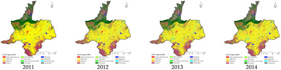
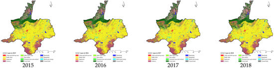
Figure 8. Spatial distribution of the predicted LULC data between 2011 and 2018.

As with the previous results, the LULC prediction between 2011 and 2018 was enforced by the historical LULC development between 2010 and 2019. Again, the results revealed that sugarcane was the most increasing LULC type, with an increasing annual rate of 17.04 km² per year, while cassava and forest land were the most decreasing LULC types, with decreasing annual change rates of 15.49 and 13.71 km² per year.

In summary, the proportional area of the time series LULC data between 2001 and 2019 based on RF classification and CLUE-S prediction is displayed in Figure 9.

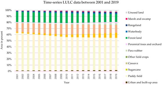
Figure 9. Proportion area of LULC type of LULC data between 2001 and 2019.

4.6. Surface Runoff Estimation between 2001 and 2010

The surface runoff estimation between 2001 and 2010 was estimated with three runoff curve number (CN) values assigned based on three different AMC conditions (see Table 3) for suitable AMC identification in the study area. In principle, the AMC is an indicator of watershed wetness and availability of soil storage. The annual surface runoff volume of the three AMC conditions with rainfall data between 2001 and 2010 is presented in Table 16 and Figure 10.

Table 16. Annual surface runoff volume of the three AMC conditions and rainfall data between 2001 and 2010.

Year	Surface Runoff Volume (million m3)			Annual Rainfall * (mm)
	AMC-I	AMC-II	AMC-III
2001	1178.41	939.70	1537.88	939.70
2002	4057.74	1191.60	4652.40	1191.60
2003	1444.46	900.80	1836.21	900.80
2004	1335.34	915.40	1716.51	915.40
2005	1754.45	1039.00	2185.22	1039.00
2006	4229.13	1196.00	4847.85	1196.00
2007	3234.72	1342.90	3795.55	1342.90
2008	5869.54	1695.20	6558.70	1695.20
2009	4189.38	1502.10	4804.03	1502.10
2010	5761.81	1506.30	6437.31	1506.30

* Annual rainfall data at Chaiyaphum meteorological station, located at the center of the study area.

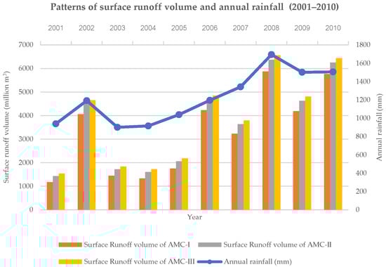
Figure 10. Patterns of surface runoff volume of the three AMC conditions and annual rainfall data between 2001 and 2010.

According to the results, the accumulated surface runoff volume under three AMC conditions was relatively different, because the CN values of these conditions were different (Table 3), while annual rainfall data were the same. The patterns of surface runoff volume under the three AMC conditions and annual rainfall between 2001 and 2010 were similar. The higher the annual rainfall, the higher the surface runoff. This finding was confirmed by simple linear regression analysis, as shown in Figure 11. The surface runoff volume under the three AMC conditions positively correlated with annual rainfall, with R² values of 0.8503, 0.8511, and 0.8513, respectively. These coefficient values show a strong relationship between annual rainfall and surface runoff, according to [50].

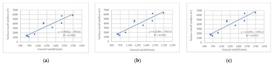
Figure 11. Relationship between surface runoff volume and annual rainfall: (a) AMC-I, (b) AMC-II, and (c) AMC-III.

In addition, the results of model performance using NSE, R², and PBIAS for identifying the suitable AMC for surface runoff estimation based on observed and simulated data between 2001 and 2010 (Table 17) are reported in Table 18.

Table 17. Annual surface runoff volume of the three AMC conditions and rainfall data between 2001 and 2010.

Year	E.21 Hydrological Station				E.23 Hydrological Station				E.6C Hydrological Station
	Qobs	AMC-I	AMC-II	AMC-III	Qobs	AMC-I	AMC-II	AMC-III	Qobs	AMC-I	AMC-II	AMC-III
		Qsim	Qsim	Qsim		Qsim	Qsim	Qsim		Qsim	Qsim	Qsim
2001	633.4	601.82	695.9	725.99	373.1	292.79	354.69	382.87	36.64	25.82	45.19	61.25
2002	1954.20	1820.05	1959.27	2001.76	1500.70	929.33	1032.16	1074.94	166.38	113.11	169.23	204.97
2003	656.7	650.03	746.73	777.44	575.6	316.3	379.93	408.74	50.63	21.6	37.64	51.78
2004	549.9	838.14	945	978.53	542.4	409.53	482.1	514.13	41.21	31.16	53.41	71.19
2005	854.7	1077.71	1195.42	1232.06	653.8	530	612.45	648.2	84.33	54.38	90.48	116.27
2006	2230.50	2439.22	2590.81	2636.54	1630.70	1246.65	1364.56	1412.19	73.37	35.22	61.22	81.35
2007	1914.30	1450.86	1581.28	1621.40	845.5	724.36	819.84	859.75	85.42	47.58	82.78	107.02
2008	3494.50	3173.60	3334.97	3383.21	1932.20	1625.72	1754.19	1804.98	180.45	146.87	214.7	256.12
2009	2180.20	2181.08	2328.33	2372.98	1560.00	1121.68	1234.52	1280.50	151.03	122.82	184.17	222.61
2010	3188.90	3033.46	3189.97	3237.17	2174.40	1570.83	1698.55	1749.15	206.15	181.51	255.45	299.02
Average	1765.73	1726.60	1856.77	1896.71	1178.84	876.72	973.3	1013.54	107.56	78.01	119.43	147.16

Table 18. Statistical data of model performance for suitable AMC identification and model validation.

AMC	Year	E.21 Station			E.23 Station			E.6C Station
		NSE	R2	PBIAS	NSE	R2	PBIAS	NSE	R2	PBIAS
AMC-II	2001	0.95	0.96	0.18	0.67	0.96	0.68	0.71	0.96	1.01
	2002			0.76			4.85			4.95
	2003			0.04			2.20			2.70
	2004			–1.63			1.13			0.93
	2005			–1.26			1.05			2.78
	2006			–1.18			3.26			3.55
	2007			2.62			1.03			3.52
	2008			1.82			2.60			3.12
	2009			–0.01			3.72			2.62
	2010			0.88			5.12			2.29
AMC-II	2001	0.94	0.96	–0.35	0.82	0.96	0.16	0.85	0.97	–0.79
	2002			–0.03			3.97			–0.27
	2003			–0.51			1.66			1.21
	2004			–2.24			0.51			–1.13
	2005			–1.93			0.35			–0.57
	2006			–2.04			2.26			1.13
	2007			1.89			0.22			0.25
	2008			0.90			1.51			–3.18
	2009			–0.84			2.76			–3.08
	2010			–0.01			4.04			–4.58
AMC-III	2001	0.94	0.96	–0.52	0.86	0.96	–0.08	0.32	0.97	–2.29
	2002			–0.27			3.61			–3.59
	2003			–0.68			1.42			–0.11
	2004			–2.43			0.24			–2.79
	2005			–2.14			0.05			–2.97
	2006			–2.30			1.85			–0.74
	2007			1.66			–0.12			–2.01
	2008			0.63			1.08			–7.03
	2009			–1.09			2.37			–6.66
	2010			–0.27			3.61			–8.63

As a result, in Table 18, under the AMC-I condition, the NSE value varied from 0.67 to 0.95, while the R² value varied from 0.71 to 0.96 (Figure 12). The PBIAS values ranged from –1.63% for overestimation to 2.62% for underestimation. Meanwhile, under the AMC-II condition, the NSE value varied from 0.86 to 0.94, while the R² value varied from 0.96 to 0.97 (Figure 13). The PBIAS values ranged from –4.58% for overestimation to 1.21% for underestimation. In the meantime, under the AMC-III condition, the NSE value varied from 0.32 to 0.96, while the R² value varies from 0.96 to 0.97 (Figure 14). The PBIAS values ranged from –8.63% to –0.11% for overestimation.

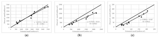
Figure 12. Relationship between the observed and estimated runoff between 2001 and 2010 under the AMC-I condition at the three stations: (a) E.21 station, (b) E.23 station, and (c) E.6C station.

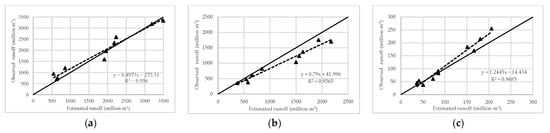
Figure 13. Relationship between the observed and estimated runoff between 2001 and 2010 under the AMC-II condition at the three stations: (a) E.21 station, (b) E.23 station, and (c) E.6C station.

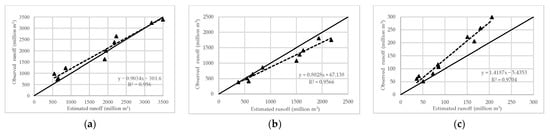
Figure 14. Relationship between the observed and estimated runoff between 2001 and 2010 under the AMC-III condition at the three stations: (a) E.21 station, (b) E.23 station, and (c) E.6C station.

These findings indicate that the NSE values under the three AMCs conditions can provide a perfect fit for surface runoff estimation. Likewise, the R² values indicate a very high correlation between the observed and estimated surface runoff for all AMC conditions. Similarly, the PBIAS values show a relatively different overestimation and underestimation among three AMC conditions less than ±10%. These results show a very good fit between the observed and estimated surface runoff for the surface runoff estimation using the SCS-CN method, as suggested by [50] (see Table 3).

Furthermore, the NSE, R², and PBIAS of all of the AMCs were compared to identify the suitable AMC for surface runoff estimation between 2011 and 2019, as shown in Table 19. As a result, AMC-II provided better overall average statistics measurements than the other AMCs. Thus, the AMC-II condition was chosen as the suitable AMC for surface runoff estimation in the second period (2011–2019).

Table 19. Comparison of the average statistics measurement for suitable AMC examination.

AMC	Average Statistics Measurement
	NSE	R2	PBIAS
AMC-I	0.7767	0.9600	1.8443
AMC-II	0.8700	0.9633	0.0423
AMC-III	0.7067	0.9633	–1.0067

4.7. Surface Runoff Estimation between 2011 and 2019

The LULC and annual rainfall data between 2011 and 2019 as dynamic input with the hydrologic soil group were applied to estimate the surface runoff with the suitable AMC-II using the Model Builder of ArcGIS (See Figure 3). The annual surface runoff volume with rainfall data between 2011 and 2019 is reported in Table 20 and Figure 15.

Table 20. Annual surface runoff volume and rainfall data between 2011 and 2019.

Year	Surface Runoff Volume (million m3)	Annual Rainfall (mm)
2011	6142.43	1428.30
2012	3583.03	1087.20
2013	4200.48	1333.30
2014	1003.60	793.50
2015	1233.80	919.30
2016	3475.16	1044.20
2017	5433.33	1281.80
2018	2588.57	809.00
2019	1445.54	752.60

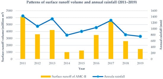
Figure 15. Pattern of surface runoff volume and annual rainfall of AMC-II between 2011 and 2019.

As a result, the surface runoff volume ranged from approximately 1004 million m³ in 2014 to approximately 6142 million m³ in 2011. The pattern of surface runoff volume and annual rainfall between 2011 and 2019 was similar. As mentioned in the previous section, the surface runoff volume positively correlated with annual rainfall, with an R² of 0.8511. This finding is consistent with previous studies [69,70].

Furthermore, the results of model performance using NSE, R², and PBIAS for validating surface runoff estimation based on observed and simulated data between 2011 and 2019 (Table 21) are reported in Table 22.

Table 21. Comparison of the observed (Q_obs) and simulated (Q_sim) surface runoff between 2011 and 2019 of the three stations.

	E.21 Station		E.23 Station		E.63 Station
Year	Qobs	Qsim	Qobs	Qsim	Qobs	Qsim
2011	2943.40	2919.23	2283.30	1954.57	175.78	158.26
2012	1989.10	1694.14	677.20	882.97	112.15	151.54
2013	1884.80	2058.57	1646.70	1492.01	70.59	79.15
2014	339.30	600.38	330.40	299.17	19.87	23.05
2015	440.80	547.04	418.70	272.62	27.32	53.76
2016	1563.30	1490.67	1058.30	771.66	87.26	75.27
2017	2732.70	2668.97	1823.20	1563.06	182.55	166.29
2018	923.60	1089.07	665.80	573.76	64.48	78.83
2019	60.10	795.50	84.20	412.55	38.25	59.31
Average	1430.79	1540.40	998.64	913.60	86.47	93.94

Note: Observed (Q_obs) and simulated (Q_sim) surface runoff in a million m³.

Table 22. Statistical model performance data for the surface runoff estimation between 2011 and 2019 at the three stations.

Year	E.21 Station			E.23 Station			E.6C Station
	NSE	R2	PBIAS	NSE	R2	PBIAS	NSE	R2	PBIAS
2011	0.91	0.94	0.19	0.90	0.94	3.66	0.87	0.90	2.25
2012			2.29			–2.29			–5.06
2013			–1.35			1.72			–1.10
2014			–2.03			0.35			–0.41
2015			–0.83			1.63			–3.40
2016			0.56			3.19			1.54
2017			0.49			2.89			2.09
2018			–1.28			1.02			–1.84
2019			–5.71			–3.65			–2.71

As a result, in Table 22, the NSE value from three stations varied from 0.87 to 0.91, with an average of 0.8933. The R² value varied from 0.87 to 0.94, with an average of 0.9033 (Figure 16). The PBIAS values ranged from –5.71% for overestimating to 3.66% for underestimating.

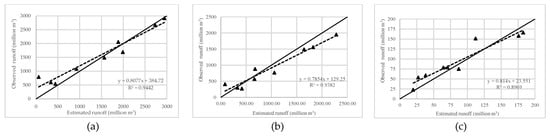
Figure 16. Relationship between the observed and estimated runoff between 2011 and 2019 at the three stations: (a) E.21 station, (b) E.23 station, and (c) E.6C station.

According to a statistical report of model performance for surface runoff estimation between 2011 and 2019, the derived NSE and R² values were more than 0.87 and the PBIAS value was less than ±10. These results show a very good fit for the surface runoff estimation with a very high correlation between the observed and estimated surface runoff, as suggested by [50] (see Table 3). Thus, it can be concluded that the surface runoff estimation using the SCS-CN method in the current study can be validated with acceptable results.

4.8. SPI Calculation for Rainfall Condition Identification

The available historical rainfall data records from 33 years (1987–2019) of the Chaiyaphum meteorological station (Figure 17) were applied to calculate the 12-month SPI index, as shown in Figure 18. The derived SPI values were classified into seven drought types and grouped into three rainfall conditions: dry, normal, and wet years, as summarized in Table 23.

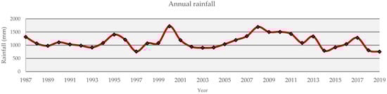
Figure 17. Annual rainfall of Chaiyaphum meteorological station (1987–2019).

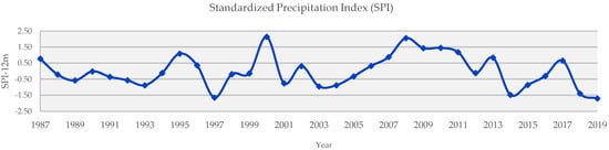
Figure 18. The 12-month SPI values of Chaiyaphum meteorological station (1987 and 2019).

Table 23. The 12-month SPI values, drought classification, and rainfall conditions of Chaiyaphum meteorological station (1987–2019).

Year	SPI	Drought Classification 1	Rainfall Conditions	Year	SPI	Drought Classification 1	Rainfall Conditions
1987	0.77	Mild wet	Wet year	2004	–0.88	Mild drought	Dry year
1988	–0.21	Near normal	Normal year	2005	–0.32	Near normal	Normal year
1989	–0.58	Mild drought	Dry year	2006	0.32	Near normal	Normal year
1990	–0.02	Near normal	Normal year	2007	0.87	Mild wet	Wet year
1991	–0.35	Near normal	Normal year	2008	2.06	Extreme wet	Wet year
1992	–0.57	Mild drought	Dry year	2009	1.43	Moderate wet	Wet year
1993	–0.88	Mild drought	Dry year	2010	1.45	Moderate wet	Wet year
1994	–0.12	Near normal	Normal year	2011	1.18	Moderate wet	Wet year
1995	1.09	Moderate wet	Wet year	2012	–0.12	Near normal	Normal year
1996	0.36	Mild wet	Wet year	2013	0.84	Mild wet	Wet year
1997	–1.65	Severe drought	Dry year	2014	–1.48	Moderate drought	Dry year
1998	–0.19	Near normal	Normal year	2015	–0.86	Mild drought	Dry year
1999	–0.14	Near normal	Normal year	2016	–0.30	Near normal	Normal year
2000	2.14	Extreme wet	Wet year	2017	0.65	Mild wet	Wet year
2001	–0.76	Mild drought	Dry year	2018	–1.40	Moderate drought	Dry year
2002	0.31	Near normal	Normal year	2019	–1.70	Severe drought	Dry year
2003	–0.95	Mild drought	Dry year

Note: ¹ SPI drought classification by [51].

As a result, the dry years were found to be 2001, 2003, 2004, 2014, 2015, 2018, and 2019. Meanwhile, normal years occurred in 2002, 2005, 2006, 2012, and 2016, and wet years in 2007, 2008, 2009, 2010, 2011, 2013, and 2017.

4.9. Optimization of LULC Allocation for Flood Mitigation

Goal programming of multi-objective decision analysis (MODA) was applied to allocate the optimum LULC to minimize surface runoff for flood mitigation based on the average surface runoff coefficient from LULC under three rainfall conditions. In this study, an average of each LULC type was separately extracted from the time series surface runoff between 2001 and 2019 for dry, normal, and wet years, as presented in Table 24.

Table 24. Runoff coefficient and its average in dry years.

No.	LULC Type	Average Surface Runoff Coefficient (million m3/km2)
		Dry Year	Normal Year	Wet Year
1	Urban and built-up areas	0.45	1.03	1.46
2	Paddy fields	0.44	1.01	1.44
3	Sugarcane	0.38	0.90	1.30
4	Cassava	0.45	1.00	1.41
5	Other field crops	0.39	0.88	1.31
6	Para rubber	0.37	0.83	1.30
7	Perennial trees and orchards	0.38	0.84	1.31
8	Forest land	0.28	0.76	1.17
9	Waterbodies	0.49	1.04	1.51
10	Rangeland	0.42	0.92	1.36
11	Marshes and swamps	0.54	1.14	1.59
12	Unused land	0.46	1.02	1.41

At the same time, the constraints of goal programming subjected to the change of LULC area in the study area were assigned for optimizing the LULC allocation for flood mitigation based on the historical LULC development between 2010 and 2019. In this study, a 10-year period was chosen to predict LULC data in 2029, 2039, and 2049 based on a period of input data (2010–2019) for transitional area prediction by the Markov Chain model. Accordingly, the changing area of each LULC type was categorized into two groups: Decreased area (paddy fields, cassava, forest land, waterbodies, rangeland, and marshes and swamps) and increased area (urban and built-up areas, sugarcane, other field crops, para rubber, perennial trees and orchards, and unused land) according to the derived transitional change area from the Markov Chain model. Details of the LULC change to minimize surface runoff in 2029, 2039, and 2049 as constraints of goal programming are summarized in Table 25.

Table 25. Existing and predicted areas of LULC in 2029, 2039, and 2049 for constraint setting.

LULC Types	Existing Area (km2)	LULC in 2029 (km2)		LULC in 2039 (km2)		LULC in 2049 (km2)
		Predicted Area	Remark	Predicted Area	Remark	Predicted Area	Remark
Urban and built-up areas (X1)	65.84	77.38	0.17% increase	88.31	0.34% increase	99.03	0.50% increase
Paddy fields (X2)	2012.16	1947.12	0.03% decrease	1879.30	0.06% decrease	1812.16	0.09% decrease
Sugarcane (X3)	306.85	424.95	0.38% increase	520.31	0.69% increase	599.36	0.95% increase
Cassava (X4)	489.91	408.26	0.16% decrease	358.65	0.26% decrease	330.32	0.32% decrease
Other field crops (X5)	6.19	7.72	0.27% increase	9.4525	0.52% increase	11.26	0.81% increase
Para rubber (X6)	97.03	134.43	0.38% increase	152.02	0.56% increase	164.41	0.69% increase
Perennial trees and orchards (X7)	88.95	125.36	0.40% increase	160.12	0.80% increase	193.13	1.17% increase
Forest land (X8)	481.30	382.63	0.20% decrease	304.44	0.36% decrease	242.23	0.49% decrease
Waterbodies (X9)	53.30	49.52	0.07% decrease	47.01	0.13% decrease	42.78	0.19% decrease
Rangeland (X10)	71.65	70.54	0.01% decrease	69.91	0.02% decrease	66.05	0.07% decrease
Marshes and swamps (X11)	27.73	25.13	0.09% decrease	24.66	0.11% decrease	21.61	0.07% decrease
Unused land (X12)	93.31	141.20	0.51% increase	180.07	0.93% increase	212.00	1.27% increase
Total	3794.22	3794.22		3794.22		3794.22

Based on the linearity of the objective function and constraints, the objective functions of the surface runoff minimization problem for optimizing LULC allocation in dry, normal, and wet years were formulated as shown in Equations (17)–(19).

$$\begin{array}{c}\mathrm{Min}\left(\mathrm{Z}\right)=0{.45\mathrm{X}}_1+0{.44\mathrm{X}}_2+0{.38\mathrm{X}}_3+0{.45\mathrm{X}}_4+0{.39\mathrm{X}}_5+0{.37\mathrm{X}}_6+0{.38\mathrm{X}}_7+0{.28\mathrm{X}}_8+0{.49\mathrm{X}}_9+\\ 0.42{\mathrm{X}}_{10}+0.54{\mathrm{X}}_{11}+0.46{\mathrm{X}}_{12}\end{array}$$

(17)

$$\begin{array}{c}\mathrm{Min}\left(\mathrm{Z}\right)=1.03{\mathrm{X}}_1+1.01{\mathrm{X}}_2+0.90{\mathrm{X}}_3+1.00{\mathrm{X}}_4+0.88{\mathrm{X}}_5+0.83{\mathrm{X}}_6+0.84{\mathrm{X}}_7+0.76{\mathrm{X}}_8+1.04{\mathrm{X}}_9+\\ 0.92{\mathrm{X}}_{10}+1.14{\mathrm{X}}_{11}+1.02{\mathrm{X}}_{12}\end{array}$$

(18)

$$\begin{array}{c}\mathrm{Min}\left(\mathrm{Z}\right)=1.46{\mathrm{X}}_1+1.44{\mathrm{X}}_2+1.30{\mathrm{X}}_3+1.41{\mathrm{X}}_4+1.31{\mathrm{X}}_5+1.30{\mathrm{X}}_6+1.31{\mathrm{X}}_7+1.17{\mathrm{X}}_8+1.51{\mathrm{X}}_9+\\ 1.36{\mathrm{X}}_{10}+1.59{\mathrm{X}}_{11}+1.41{\mathrm{X}}_{12}\end{array}$$

(19)

The constraints for optimizing LULC allocation in 2029, 2039, and 2049 to minimize runoff under three rainfall conditions using objective functions (Equations (17)–(19)) are summarized in Table 26. Additionally, two mandatory constraints, as described by Equations (11) and (14) in Section 3.5.2, were set under the three rainfall conditions as follows:

Table 26. Summary of the constraint setting for each LULC type in 2029, 2039, and 2049.

LULC Types	Constraints Setting for Each LULC Type
	Constrain in 2029	Constrain in 2039	Constrain in 2049
Urban and built-up areas (X1)	65.84 ≤ X1 ≤ 77.38	65.84 ≤ X1 ≤ 88.31	65.84 ≤ X1 ≤ 99.03
Paddy fields (X2)	2012.16 ≥ X2 ≥ 1947.12	2012.16 ≥ X2 ≥ 1879.30	2012.16 ≥ X2 ≥ 1812.16
Sugarcane (X3)	306.85 ≤ X3 ≤ 424.95	306.85 ≤ X3 ≤ 520.31	306.85 ≤ X3 ≤ 599.36
Cassava (X4)	489.91 ≥ X4 ≥ 408.26	489.91 ≥ X4 ≥ 358.65	489.91 ≥ X4 ≥ 330.32
Other field crops (X5)	6.19 ≤ X5 ≤ 7.72	6.19 ≤ X5 ≤ 9.45	6.19 ≤ X5 ≤ 11.26
Para rubber (X6)	97.03 ≤ X6 ≤ 134.43	97.03 ≤ X6 ≤ 152.02	97.03 ≤ X6 ≤ 164.41
Perennial trees and orchards (X7)	88.95 ≤ X7 ≤ 125.36	88.95 ≤ X7 ≤ 160.12	88.95 ≤ X7 ≤ 193.13
Forest land (X8)	481.30 ≥ X8 ≥ 382.63	481.30 ≥ X8 ≥ 304.44	481.30 ≥ X8 ≥ 242.23
Waterbodies (X9)	53.30 ≥ X9 ≥ 49.52	53.30 ≥ X9 ≥ 47.01	53.30 ≥ X9 ≥ 42.78
Rangeland (X10)	71.65 ≥ X10 ≥ 70.54	71.65 ≥ X10 ≥ 69.91	71.65 ≥ X10 ≥ 66.05
Marshes and swamps (X11)	27.73 ≥ X11 ≥ 25.13	27.73 ≥ X11 ≥ 24.66	27.73 ≥ X11 ≥ 21.61
Unused land (X12)	93.31 ≤ X12 ≤ 141.20	93.31 ≤ X12 ≤ 180.07	93.31 ≤ X12 ≤ 211.89

The first mandatory constraint, related to the area of all land use classes, must be equal to the allowable area of 3794.22 km², as shown in Equation (20).

$${\mathrm{X}}_1{+\mathrm{X}}_2{+\mathrm{X}}_3{+\mathrm{X}}_4{+\mathrm{X}}_5{+\mathrm{X}}_6{+\mathrm{X}}_7{+\mathrm{X}}_8{+\mathrm{X}}_9{+\mathrm{X}}_{10}{+\mathrm{X}}_{11}{+\mathrm{X}}_{12}=3794.22$$

(20)

The second mandatory constraint is related to the non-negative variable. The area of each land use class should be more than or equal to 0 km², as shown in Equation (21).

$${\mathrm{X}}_1{+\mathrm{X}}_2{+\mathrm{X}}_3{+\mathrm{X}}_4{+\mathrm{X}}_5{+\mathrm{X}}_6{+\mathrm{X}}_7{+\mathrm{X}}_8{+\mathrm{X}}_9{+\mathrm{X}}_{10}{+\mathrm{X}}_{11}{+\mathrm{X}}_{12}\ge 0$$

(21)

The objective functions for dry, normal, and wet years (Equations (17)–(19)) were then transformed into a goal programming form as follows:

$${\mathrm{f}}_{\mathrm{k}}\left(\mathrm{x}\right)+{\mathrm{d}}_{\mathrm{k}}^{-}-{\mathrm{d}}_{\mathrm{k}}^{+}{=\mathrm{a}}_{\mathrm{k}}$$

(22)

The results of the optimized LULC allocation to minimize surface runoff for flood mitigation in 2029, 2039, and 2049 under the three rainfall conditions (dry, normal, and wet years) are presented in Table 27, Table 28 and Table 29.

Table 27. Optimization of LULC allocation to minimize surface runoff in dry years.

LULC Types	2019		2029		2039		2049
	Area of LULC	Surface Runoff	Allocated LULC	Surface Runoff	Allocated LULC	Surface Runoff	Allocated LULC	Surface Runoff
Urban and built-up areas	65.84	29.84	65.84	29.84	65.84	29.84	65.84	29.84
Paddy fields	2012.16	942.32	1947.12	856.54	1879.30	826.71	1812.16	797.17
Sugarcane	306.85	70.96	387.24	148.87	454.94	174.90	517.13	198.81
Cassava	489.91	242.89	408.26	184.27	359.65	162.33	330.32	149.09
Other field crops	6.19	1.75	6.19	2.39	6.19	2.39	6.19	2.39
Para rubber	97.03	19.65	134.43	49.86	152.02	56.39	164.41	60.99
Perennial trees and orchards	88.95	25.76	125.36	47.40	160.12	60.54	193.13	73.02
Forest land	481.30	159.21	481.30	136.03	481.30	136.03	481.30	136.03
Waterbodies	53.30	23.81	49.52	24.29	47.01	23.06	42.78	20.99
Rangeland	71.65	23.23	70.54	29.36	69.91	29.10	66.05	27.49
Marshes and swamps	27.73	12.69	25.13	13.59	24.66	13.34	21.61	11.69
Unused land	93.31	25.85	93.31	42.57	93.31	42.57	93.31	42.57
Total	3794.22	1577.96	3794.22	1565.01	3794.22	1557.18	3794.22	1550.07

Note: Area of LULC in kilometers squared, surface runoff in million meters cubed, and allocated LULC in kilometers squared.

Table 28. Optimization of LULC allocation to minimize surface runoff in normal years.

LULC Types	2019		2029		2039		2049
	Area of LULC	Surface Runoff	Allocated LULC	Surface Runoff	Allocated LULC	Surface Runoff	Allocated LULC	Surface Runoff
Urban and built-up areas	65.84	67.58	65.84	67.58	65.84	67.58	65.84	67.58
Paddy fields	2012.16	2038.95	1947.12	1973.05	1879.30	1904.33	1812.16	1836.29
Sugarcane	306.85	277.30	385.71	348.56	451.67	408.18	512.06	462.76
Cassava	489.91	489.07	408.26	407.56	359.65	359.03	330.32	329.75
Other field crops	6.19	5.43	7.72	6.78	9.45	8.30	11.26	9.88
Para rubber	97.03	80.36	134.43	111.33	152.02	125.89	164.41	136.16
Perennial trees and orchards	88.95	74.28	125.36	104.68	160.12	133.70	193.13	161.27
Forest land	481.30	366.03	481.30	366.03	481.30	366.03	481.30	366.03
Waterbodies	53.30	55.23	49.52	51.30	47.01	48.70	42.78	44.33
Rangeland	71.65	65.95	70.54	64.93	69.91	64.35	66.05	60.80
Marshes and swamps	27.73	31.56	25.13	28.60	24.66	28.06	21.61	24.59
Unused land	93.31	95.33	93.31	95.33	93.31	95.33	93.31	95.33
Total	3794.22	3647.07	3794.22	3625.72	3794.22	3609.48	3794.22	3594.76

Note: Area of LULC in kilometers squared, surface runoff in million meters cubed, and allocated LULC in kilometers squared.

Table 29. Optimization of LULC allocation to minimize surface runoff in wet years.

LULC Types	2019		2029		2039		2049
	Area of LULC	Surface Runoff	Allocated LULC	Surface Runoff	Allocated LULC	Surface Runoff	Allocated LULC	Surface Runoff
Urban and built-up areas	65.84	95.82	65.84	95.82	65.84	95.82	65.84	95.82
Paddy fields	2012.16	2889.20	1947.12	2795.81	1879.30	2698.43	1812.16	2602.02
Sugarcane	306.85	400.38	422.14	552.77	520.31	678.91	599.36	782.05
Cassava	489.91	688.86	408.26	574.05	358.65	505.70	330.32	464.46
Other field crops	6.19	8.09	6.19	8.09	9.45	12.36	11.26	14.71
Para rubber	97.03	126.18	134.43	174.82	152.02	197.69	164.41	213.81
Perennial trees and orchards	88.95	116.42	88.95	116.42	90.48	119.73	103.83	138.51
Forest land	481.30	563.35	481.30	563.35	481.30	563.35	481.30	563.35
Waterbodies	53.30	80.24	50.02	74.55	48.01	70.77	43.78	64.41
Rangeland	71.65	97.12	70.54	95.60	69.91	94.76	66.05	89.52
Marshes and swamps	27.73	44.10	26.13	39.97	25.66	39.21	22.61	34.37
Unused land	93.31	131.74	93.31	131.74	93.31	131.74	93.31	131.74
Total	3794.22	5241.52	3794.22	5223.01	3794.22	5208.46	3794.22	5194.79

Note: Area of LULC in kilometers squared, surface runoff in million meters cubed, and allocated LULC in kilometers squared.

In dry years, the significant increasing LULC type after optimizing LULC allocation in 2029, 2039, and 2049 were sugarcane, with approximately 80, 148, and 210 km². In contrast, the significantly decreasing LULC type was cassava, with approximately 82, 133, and 200 km². Additionally, the annual surface runoff decreased in 2029, 2039, and 2049 by 12.95, 20.78, and 27.89 million m³, or approximately 0.82%, 1.32%, and 1.77% of total estimated surface runoff in 2019 (See Table 27).

Meanwhile, the most increased LULC area under the normal year was also sugarcane, with an area of approximately 79, 145, and 205 km². In contrast, the significant decreasing LULC types were paddy fields, with approximately 65, 133, and 200 km², and sugarcane, with an area of approximately 82, 130, and 160 km². Additionally, the annual surface runoff decreased in 2029, 2039, and 2049 by 21.34, 37.59, and 52.31 million m³, or 0.59%, 1.03%, and 1.43% of the total estimated surface runoff in 2019 (see Table 28).

In the meantime, the most increasing LULC type in wet years was sugarcane, with an area of approximately 115, 213, and 293 km², respectively. Conversely, the significant decreasing LULC types were paddy fields, with approximately 65, 133, and 200 km², and sugarcane, with approximately 82, 131, and 160 km². Additionally, the annual surface runoff decreased in 2029, 2039, and 2049 by 18.52, 33.06, and 46.73 million m³, or approximately 0.35%, 0.63%, and 0.89% from the total estimated surface runoff in 2019 (see Table 29).

According to these results, the optimized LULC allocation data in 2049 of the dry, normal and wet years were suitable for flood mitigation according to surface runoff reduction. The surface runoff under dry, normal and wet years in 2049 reduced by approximately 27.89, 52.31, and 46.73 million m³ (Figure 19).

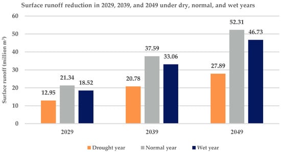
Figure 19. Surface runoff reduction in 2029, 2039, and 2049 in dry, normal, and wet years.

Moreover, notable reductions in annual surface runoff under the three rainfall conditions occurred in paddy fields and cassava to sugarcane, para rubber, and perennial trees and orchards after optimization, which changed the hydrological properties. Paddy and cassava fields provided higher runoff coefficients than sugarcane, rubber, and perennial trees and orchards (see Table 27, Table 28 and Table 29). This finding is consistent with previous studies [19,20,71].

The deviation in annual surface runoff after minimization by goal programming is presented in Table 30. As a result, the percentage deviation from the goal varied from –1.77% to –0.35%, which is acceptable.

Table 30. Deviation of annual surface runoff after minimization by goal programming.

Items	Surface Runoff Minimization (million m3)
	Dry Years			Normal Years			Wet Years
	2029	2039	2049	2029	2039	2049	2029	2039	2049
Goal of annual surface runoff (million m3)	1577.96	1577.96	1577.96	3647.07	3647.07	3647.07	5241.52	5241.52	5241.52
Annual surface runoff after optimization (million m3)	1565.01	1557.18	1550.07	3625.72	3609.48	3594.76	5223.01	5208.46	5194.79
Deviation from goal (million m3)	–12.95	–20.78	–27.89	–21.34	–37.59	–52.31	–18.52	–33.06	–46.73
Deviation from goal (%)	–0.82	–1.32	–1.77	–0.59	–1.03	–1.43	–0.35	–0.63	–0.89

4.10. Mapping of LULC Allocation for Flood Mitigation

LULC data in 2019 and the derived optimum local parameter of the CLUE-S model were applied to map the suitable LULC allocation to minimize surface runoff for flood mitigation in 2049 of the three rainfall conditions. The conversion matrix for each possible LULC type change in 2049 was based on transitional LULC change between 2010 and 2019, as shown in Table 31. Meanwhile, the elasticity values were assigned based on the transition probability matrix of LULC change between 2019 and 2049 from the Markov Chain model, as shown in Table 32. Thus, the elasticity values of the urban and built-up areas, paddy fields, sugarcane, cassava, other field crops, para rubber, perennial trees and orchards, forest land, waterbodies, rangeland, marshes and swamps, and unused land for LULC prediction in 2049 were 1.00, 0.83, 0.83, 0.31, 0.97, 0.52, 0.96, 0.70, 0.76, 0.71, 0.76, and 0.87, respectively.

Table 31. Conversion matrix of the possible change in 2029, 2039, and 2049.

	LULC Types	LULC Type Possible Change in 2029, 2039, and 2049
		UR	PA	SU	CA	FC	PR	PO	FO	WA	RA	MA	UL
LULC in 2019	Urban and built-up areas (UR)	1	0	0	0	0	0	0	0	0	0	0	0
	Paddy fields (PA)	0	1	1	1	0	0	0	0	0	1	1	0
	Sugarcane (SU)	1	0	1	1	0	1	1	0	0	0	0	0
	Cassava (CA)	1	1	1	1	0	1	1	0	0	1	0	1
	Other field crops (FC)	0	0	0	0	1	0	0	0	0	0	0	0
	Para rubber (PR)	0	0	1	1	1	1	0	0	0	0	0	1
	Perennial trees and orchards (PO)	0	0	1	1	0	0	1	0	0	0	0	0
	Forest land (FO)	0	0	0	0	0	1	1	1	0	1	0	1
	Waterbodies (WA)	0	0	0	0	0	0	0	0	1	0	1	0
	Rangeland (RA)	0	1	0	1	0	0	1	0	0	1	0	0
	Marshes and swamps (MA)	0	1	1	0	0	0	1	0	0	0	1	0
	Unused land (UL)	1	0	0	0	0	0	0	0	0	0	0	1

Table 32. Elasticity of LULC change for LULC prediction between 2019 and 2049.

	LULC Typess	LULC Type Possible Change in 2049
		UR	PA	SU	CA	FC	PR	PO	FO	WA	RA	MA	UL
LULC in 2019	Urban and built-up areas (UR)	1.00	-	-	-	-	-	-	-	-	-	-	-
	Paddy fields (PA)	-	0.83	0.08	0.04	-	-	0.03	-	-	-	0.01	-
	Sugarcane (SU)	0.02	0.03	0.83	0.09	-	0.01	0.02	-	-	-	-	0.01
	Cassava (CA)	0.03	0.12	0.31	0.31	-	0.11	0.03	-	-	0.01	-	0.08
	Other field crops (FC)	-	-	-	-	0.97	-	0.02	-	-	-	-	-
	Para rubber (PR)	0.01	0.02	0.05	0.18	0.02	0.52	0.07	-	-	-	-	0.13
	Perennial trees and orchards (PO)	-	0.01	0.02	0.01	-	-	0.96	-	-	-	-	-
	Forest land (FO)	0.01	0.01	0.03	0.04	-	0.10	0.04	0.70	-	0.01	-	0.04
	Waterbodies (WA)	0.01	0.10	0.07	0.03	-	-	0.01	-	0.76	-	0.01	-
	Rangeland (RA)	-	0.21	0.02	0.03	-	-	0.02	-	-	0.71	-	-
	Marshes and swamps (MA)	0.01	0.06	0.08	0.03	-	-	0.05	-	-	-	0.77	-
	Unused land (UL)	0.02	0.08	0.01	0.01	-	-	0.01	-	-	-	-	0.87

In addition, the optimized LULC allocation in 2049 in dry, normal, and wet years (see Table 27, Table 28 and Table 29) was applied to calculate the annual land requirement between 2019 and 2049 for LULC prediction.

The spatial distribution of the LULC allocation maps in 2049 for dry, normal, and wet years is displayed in Figure 20. Meanwhile, the area and percentage of LULC type in 2049 for dry, normal, and wet years are summarized in Table 33. The derived map of suitable LULC allocation to minimize surface runoff for flood mitigation of dry, normal, and wet years was further applied to evaluate economic and ecosystem service values and change.

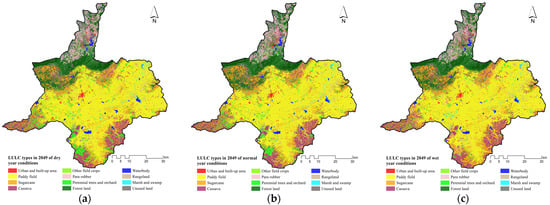
Figure 20. Spatial distribution of predicted LULC data in 2049: (a) Dry years, (b) normal years, and (c) wet years.

Table 33. Area and percentage of optimized LULC allocation to mitigate flood in 2049 in dry, normal, and wet years.

LULC Type	Dry Year		Normal Year		Wet Year
	Area (km2)	Percentage	Area (km2)	Percentage	Area (km2)	Percentage
Urban and built-up areas	65.84	1.74	65.84	1.74	65.84	1.74
Paddy fields	1812.14	47.76	1812.14	47.76	1812.18	47.76
Sugarcane	517.12	13.63	517.12	13.63	599.34	15.80
Cassava	330.33	8.71	330.33	8.71	330.34	8.71
Other field crops	6.19	0.16	6.19	0.16	11.25	0.30
Para rubber	164.42	4.33	164.42	4.33	164.41	4.33
Perennial trees and orchards	193.17	5.09	193.17	5.09	103.88	2.74
Forest land	481.26	12.68	481.26	12.68	481.3	12.69
Waterbodies	42.77	1.13	42.77	1.13	43.78	1.15
Rangeland	66.07	1.74	66.07	1.74	66.01	1.74
Marshes and swamps	21.57	0.57	21.57	0.57	22.56	0.59
Unused land	93.3	2.46	93.3	2.46	93.28	2.46
Total	3794.22	100.00	3794.22	100.00	3794.22	100.00

4.11. Economic Value Evaluation and Change

The actual LULC data in 2019 and suitable LULC data in 2049 for flood mitigation in dry, normal, and wet years (Table 34) were applied to evaluate future economic values using the PV model (Table 35), and the results are shown in Table 36 and Figure 21.

Table 34. Areas of actual LULC in 2019 and suitable LULC allocation for flood mitigation in 2049 in dry, normal, and wet years.

No.	LULC Type	Actual LULC 2019	Suitable LULC Allocation in 2049 (km2)
			Dry Years	Normal Years	Wet Years
1	Urban and built-up areas	65.84	65.84	65.84	65.84
2	Paddy fields	2012.16	1812.14	1812.13	1812.18
3	Sugarcane	306.85	517.12	512.07	599.34
4	Cassava	489.91	330.33	330.33	330.34
5	Other field crops	6.19	6.19	11.27	11.25
6	Para rubber	97.03	164.42	164.41	164.41
7	Perennial trees and orchards	88.95	193.17	193.15	103.88
8	Forest land	481.30	481.26	481.30	481.30
9	Waterbodies	53.30	42.77	42.80	43.78
10	Rangeland	71.65	66.07	66.04	66.01
11	Marshes and swamps	27.73	21.57	21.58	22.56
12	Unused land	93.32	93.30	93.28	93.28
Total		3794.22	3794.22	3794.22	3794.22

Table 35. Present and future economic value of agricultural and forest land.

LULC Type	Price (Baht/ton)	Yield (ton/km2)	Present Value (Baht/ km2)	Discount Rate 5 (%)	Future Value in 2049 Using PV Model (Baht/km2)
Paddy field 1	13,287.75	218.75	2,906,695.31	6.50	19,225,947.12
Sugarcane 2	900.00	4468.75	4,021,875.00	6.50	26,602,153.91
Cassava 1	1430.00	2240.63	3,204,093.75	6.50	21,193,049.28
Other field crops 1	8092.50	415.63	3,363,445.31	6.50	22,247,058.87
Para rubber 3	43,685.83	131.25	5,733,765.63	6.50	37,925,225.34
Perennial trees and orchard 1	25,600.00	247.24	6,329,440.00	6.50	41,865,233.77
Forest land 4	-	-	25,000,000.00	6.50	165,359,154.08

Source: ¹ [72], ² [73], ³ [74], ⁴ [75], and ⁵ discount rate was based on the minimum retail rate of Bank for [76].

Table 36. Economic value by LULC types of actual LULC 2019 and suitable LULC allocation for flood mitigation in 2049.

LULC Type	Economic Value in 2049 (Baht)
	Actual LULC in 2019	Suitable LULC Allocation for Flood Mitigation in 2049
		Dry Year	Normal Year	Wet Year
Paddy fields	38,654.20	34,629.20	34,822.30	34,826.09
Sugarcane	8147.42	13,678.87	13,614.03	15,920.81
Cassava	10,347.30	6783.21	6979.08	6968.65
Other field crops	137.81	136.47	200.36	200.68
Para rubber	3675.10	6145.56	6235.43	6222.15
Perennial trees and orchards	3717.46	9041.53	8055.82	4404.83
Forest land	79,388.71	78,164.79	79,303.89	79,315.05
Total in million Baht	144,068.00	148,579.64	149,210.92	147,858.27

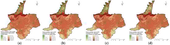
Figure 21. Spatial distribution of economic value in 2049: (a) Actual LULC 2019, (b) dry years, (c) normal years, and (d) wet years.

According to results, the top three dominant LULC types of actual LULC data in 2019 were paddy fields, cassava, and forest land, while the top three dominant LULC types of suitable LULC allocation data in 2049 for flood mitigation in dry, normal, and wet years were paddy field, sugarcane, and forest land. Moreover, the top three highest future values were forest land, perennial trees and orchards, and para rubber (Table 35).

As a result, in Table 36, the suitable LULC allocation data for flood mitigation in normal years provided the highest economic value, approximately 149,211 million Baht. In contrast, the actual LULC allocation in 2019 provided the lowest economic value, approximately 144,068 million Baht. The contribution of the economic value by LULC type from the actual LULC and suitable LULC allocation data for flood mitigation from three rainfall conditions are displayed in Figure 22.

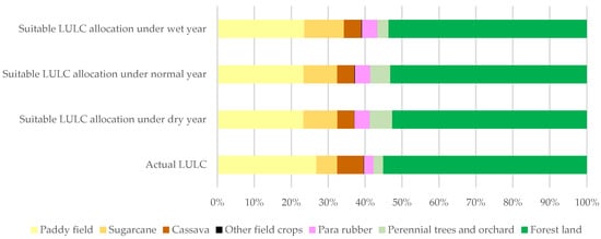
Figure 22. Contribution of the future economic value of LULC type of actual LULC and suitable LULC allocation for flood mitigation (dry, normal, and wet years).

According to the data in Figure 22, the top three dominant LULC types of actual LULC in 2019, including paddy fields, cassava, and forest land, will provide future economic value in 2049, about 89% of the total value. Meanwhile, the top three dominant LULC types of suitable LULC allocation for flood mitigation under dry, normal, and wet years, including paddy fields, sugarcane, and forest land, deliver future economic value in 2049 of approximately 85%, 86%, and 88% of the total value, respectively.

Moreover, the future economic value of forest land from actual LULC and suitable LULC allocation data for flood mitigation (dry, normal, and wet years) contributed the highest values compared to the other LULC types because the present economic value, approximately 25,000,000 Baht per km², or the future economic value, approximately 165,359,154 Baht per km², was exceptionally high when compared to other LULC types (see Table 35).

Furthermore, the results of the future economic value change by comparing the values of actual LULC data and each suitable LULC allocation for flood mitigation (dry, normal, and wet years) in terms of gain (+sign) and loss (-sign) are reported in Table 37, Table 38 and Table 39 and spatially displayed in Figure 23.

Table 37. Future economic value change in 2049 between actual LULC in 2019 and suitable LULC allocation in dry years.

	LULC Type	Suitable LULC Allocation in 2049 of Dry Years							Total
		PA	SU	CA	FC	PR	PO	FO
Actual LULC in 2019	Paddy fields (PA)	0	1507.30	28.21	0.02	18.11	602.05	1656.23	3811.92
	Sugarcane (SU)	–188.27	0	–105.11	–0.99	14.05	173.00	790.00	682.69
	Cassava (CA)	–28.21	207.96	0	0.28	813.50	1983.53	1249.23	4226.29
	Other field crops (FC)	–0.01	0.91	–0.11	0	12.19	0.42	104.33	117.73
	Para rubber (PR)	0	–2.68	–25.43	–8.99	0	2.45	1167.21	1132.55
	Perennial trees and orchards (PO)	–193.53	–123.84	–86.03	–0.35	–5.10	0	237.52	–171.32
	Forest land (FO)	–131.26	–2240.87	–630.19	–95.31	–2467.68	–305.09	0	–5870.41
	Total	–541.27	–651.22	–818.66	–105.34	–1614.92	2456.36	5204.51	3929.45

Table 38. Future economic value change in 2049 between actual LULC in 2019 and suitable LULC allocation in normal years.

	LULC Type	Suitable LULC Allocation in 2049 of Normal Years							Total
		PA	SU	CA	FC	PR	PO	FO
Actual LULC in 2019	Paddy fields (PA)	0	1453.48	28.90	0.02	38.03	563.56	1656.23	3740.22
	Sugarcane (SU)	–190.75	0	–108.03	–1.06	21.53	151.87	790.00	663.57
	Cassava (CA)	–29.13	224.39	0	0.59	975.32	1546.54	1252.86	3970.57
	Other field crops (FC)	–0.01	0.94	–0.11	0	12.05	0.41	104.46	117.74
	Para rubber (PR)	0	–2.69	–26.55	–41.85	0	2.45	1206.43	1137.79
	Perennial trees and orchards (PO)	–196.66	–123.25	–88.76	–0.64	–6.05	0	237.74	–177.62
	Forest land (FO)	–152.56	–2237.12	–645.50	–142.20	–1666.34	–286.86	0	–5130.59
	Total	–569.12	–684.25	–840.06	–185.14	–625.45	1977.96	5247.72	4321.67

Table 39. Future economic value change in 2049 between actual LULC in 2019 and suitable LULC allocation in wet years.

	LULC Type	Suitable LULC Allocation in 2049 of the Wet Year							Total
		PA	SU	CA	FC	PR	PO	FO
Actual LULC in 2019	Paddy fields (PA)	0	1525.95	27.55	0.02	58.57	323.42	1656.23	3591.74
	Sugarcane (SU)	–190.82	0	–105.43	–1.06	19.27	97.94	790.00	609.90
	Cassava (CA)	–29.16	565.99	0	0.59	971.75	245.81	1252.86	3007.84
	Other field crops (FC)	-0.01	0.95	–0.12	0	11.92	0.35	104.46	117.55
	Para rubber (PR)	0	–2.69	–31.35	–41.89	0	2.45	1206.89	1133.40
	Perennial trees and orchards (PO)	–196.68	–141.72	–90.29	–0.64	–6.21	0	237.74	–197.81
	Forest land (FO)	–152.83	–2360.51	–653.55	–143.61	–1569.08	–259.19	0	–5138.76
	Total	–569.50	–412.03	–853.19	–186.59	–513.78	410.78	5248.17	3123.86

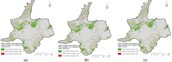
Figure 23. Gain and loss of future economic value of suitable LULC allocation for flood mitigation in 2049: (a) Dry years, (b) normal years, and (c) wet years.

According to change detection, suitable LULC allocation for flood mitigation in 2049 in normal years gained the highest future economic value of approximately 4322 million Baht (Table 38). On the contrary, suitable LULC allocation for flood mitigation in 2049 in wet years gained the highest future economic value of approximately 3124 million Baht (Table 39). These results show the consequence of LULC allocation for flood mitigation in 2049 using goal programming on future economic value, because the future economic value depends on the areas of LULC type and their values.

4.12. Ecosystem Service Value Evaluation and Change

The actual LULC data in 2019 and the suitable LULC data in 2049 for flood mitigation under dry, normal, and wet years (Table 40) were applied to evaluate the ecosystem service values using a simple benefit transfer method according to a coefficient value of LULC type (see Table 4), and the results are shown in Table 41 and Figure 24.

Table 40. Area of each LULC type for ESV evaluation of actual LULC and suitable LULC allocation for flood mitigation under dry, normal, and wet years.

No.	ESV-LULC Type	Actual LULC 2019	Suitable LULC Allocation in 2049
			Dry Years	Normal Years	Wet Years
1	Urban and built-up areas	65.84	65.84	65.84	65.84
2	Paddy fields	2012.16	1812.16	1812.16	1812.16
3	Field crop	802.95	853.64	853.64	940.94
4	Forest land	667.28	838.84	838.84	749.54
5	Waterbodies	53.3	42.78	42.78	43.78
6	Rangeland	71.65	66.05	66.05	66.05
7	Marshes and swamps	27.73	21.61	21.61	22.61
8	Unused land	93.32	93.31	93.31	93.31
Total		3794.22	3794.22	3794.22	3794.22

Table 41. Ecosystem service value by ESV-LULC types of actual LULC 2019 and suitable LULC allocation for flood mitigation in 2049.

ESV-LULC Type	Ecosystem Service Value (Baht)
	Actual LULC in 2019	Suitable LULC Allocation for Flood Mitigation in 2049
		Dry Years	Normal Years	Wet Years
Urban and built-up areas (UR)	2.60	2.62	2.62	2.62
Paddy fields (PA)	6478.73	5804.11	5836.47	5837.11
Field crops (FC)	2580.20	2708.13	2739.31	3017.20
Forest land (FO)	4050.69	5175.68	5088.76	4556.47
Waterbodies (WA)	1143.07	1019.07	923.23	951.98
Rangeland (RA)	180.65	176.46	167.47	163.55
Marshes and swamps (MA)	810.57	567.00	642.80	679.99
Unused land (UL)	27.92	27.94	27.94	27.94
Total in million Baht	15,274.42	15,481.00	15,428.61	15,236.86

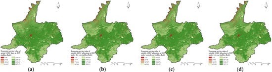
Figure 24. Spatial distribution of the ecosystem service value: (a) Actual LULC 2019, (b) dry years, (c) normal years, and (d) wet years.

As a result, the ESV of actual LULC in 2019 and the suitable LULC allocation for flood mitigation in 2049 in dry, normal, and wet years are slightly different. The suitable LULC allocation for flood mitigation in 2049 under the dry year provided the highest ESV, approximately 15,481 million Baht, while the suitable LULC allocation for flood mitigation in 2049 in wet years delivered the lowest ESV, approximately 15,237 million Baht. The contributions of ESV of each LULC type from actual LULC in 2019 and the suitable LULC allocation for flood mitigation in 2049 under the three rainfall conditions are compared in Figure 25.

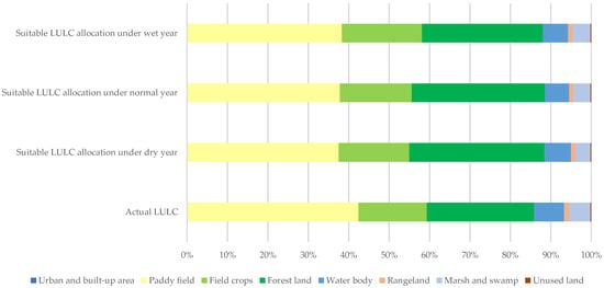
Figure 25. Contribution of the ecosystem service value of each LULC type of actual LULC and suitable LULC allocation for flood mitigation (dry, normal, and wet years).

As shown in Figure 25, paddy fields provided the highest ESV value from the actual LULC and the suitable LULC allocation data for flood mitigation in 2049 under the three rainfall conditions, because paddy fields were the most dominant type in the area. Additionally, the top three dominant LULC types, namely, paddy fields, field crops, and forest land, delivered ESVs of approximately 86%, 88%, 89%, and 88% of the total value.

Furthermore, the results of the ESV change upon comparison between values of actual LULC data and each suitable LULC allocation for flood mitigation (dry, normal, and wet years) in terms of gain (+sign) and loss (-sign) are reported in Table 42, Table 43 and Table 44 and spatially displayed in Figure 26.

Table 42. Ecosystem service value change between actual LULC in 2019 and suitable LULC allocation in 2049 in dry years.

	LULC Type	Suitable LULC Allocation in 2049 of Dry Years								Total
		UR	PA	FC	FO	WA	RA	MA	UL
Actual LULC in 2019	Urban and built-up areas (UR)	0	33.07	14.03	14.06	4.88	0.17	2.05	0.08	68.34
	Paddy fields (PA)	–36.36	0	0	111.30	40.04	–10.79	119.19	–1.86	221.52
	Field crops (FC)	–14.69	0	0	495.14	16.80	–3.06	5.11	–18.86	480.44
	Forest land (FO)	–9.60	–27.03	–102.47	0	13.13	–3.09	0.65	–91.86	–220.28
	Waterbodies (WA)	–4.93	–46.67	–15.46	–20.49	0	–0.14	39.86	–0.82	–48.65
	Rangeland (RA)	–0.16	8.88	4.30	12.49	0.19	0	0.75	–0.02	26.42
	Marshes and swamps (MA)	–1.97	–184.81	–6.07	–249.41	–0.91	–1.64	0	0	–444.81
	Unused land (UL)	–0.07	1.28	8.82	112.93	0.63	0.01	0	0	123.60
Total		–67.79	–215.28	–96.84	476.01	74.76	–18.53	167.60	–113.35	206.58

Table 43. Ecosystem service value change between the actual LULC in 2019 and the suitable LULC allocation in 2049 in normal years.

	LULC Types	Suitable LULC Allocation in 2049 of Normal Years								Total
		UR	PA	FC	FO	WA	RA	MA	UL
Actual LULC in 2019	Urban and built-up areas (UR)	0	33.21	14.25	13.47	4.68	0.15	2.18	0.08	68.02
	Paddy fields (PA)	–36.36	0	0	109.49	31.33	–10.30	119.54	–1.86	211.83
	Field crops (FC)	–14.69	0	0	460.30	16.74	–2.72	4.87	–18.86	445.63
	Forest land (FO)	–9.60	–27.85	–110.14	0	13.13	–2.75	0.65	–91.86	–228.41
	Waterbodies (WA)	–4.93	–46.67	–16.38	–19.96	0	–0.14	70.47	–0.82	–18.44
	Rangeland (RA)	–0.16	8.98	4.27	20.19	0.15	0	0.77	–0.02	34.19
	Marshes and swamps (MA)	–1.97	–184.81	–54.01	–238.61	–0.69	–1.64	0	0	–481.73
	Unused land (UL)	–0.07	1.32	9.31	111.90	0.63	0.01	0	0	123.09
Total		–67.79	–215.81	–152.70	456.77	65.98	–17.39	198.47	–113.35	154.18

Table 44. Ecosystem service value change between the actual LULC in 2019 and the suitable LULC allocation in 2049 in wet years.

	LULC Types	Suitable LULC Allocation in 2049 of Wet Years								Total
		UR	PA	FC	FO	WA	RA	MA	UL
Actual LULC in 2019	Urban and built-up areas (UR)	0	33.22	15.59	10.91	4.76	0.14	2.10	0.08	66.81
	Paddy fields (PA)	–36.36	0	0	82.27	34.28	–10.04	130.26	–1.86	198.55
	Field crops (FC)	–14.69	0	0	268.93	16.79	–2.64	3.65	–18.86	253.17
	Forest land (FO)	–9.60	–27.85	–117.37	0	13.13	–2.62	0.85	–91.86	–235.33
	Waterbodies (WA)	–4.93	–46.67	–19.20	–17.57	0	–0.14	61.42	–0.82	–27.92
	Rangeland (RA)	–0.16	8.99	4.68	21.78	0.15	0	0.72	–0.02	36.14
	Marshes and swamps (MA)	–1.97	–184.81	–214.16	–48.07	–0.76	–1.64	0	0	–451.40
	Unused land (UL)	–0.07	1.32	10.00	110.52	0.63	0.01	0	0	122.41
Total		–67.79	–215.81	–320.47	428.78	68.99	–16.92	199.01	–113.35	–37.56

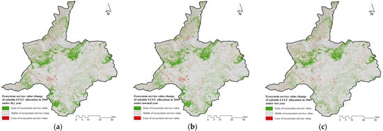
Figure 26. Gain and loss of ESV of suitable LULC allocation for flood mitigation in 2049: (a) Dry years, (b) normal years, and (c) wet years.

According to the results in Table 42, Table 43 and Table 44, the suitable LULC allocation for flood mitigation in 2049 under dry years gained the highest ESV of approximately 207 million Baht. On the contrary, the suitable LULC allocation for flood mitigation in 2049 in wet years resulted in losses in ESV of approximately 38 million Baht. These findings indicate that the ESV of suitable LULC allocation for flood mitigation in 2049 in wet years is lower than the actual LULC in 2019 (see Table 45). Similar to the change in future economic value, these results show the consequence of LULC allocation for flood mitigation in 2049 using goal programming on ESV, because the ESV depends on areas of LULC type and their coefficient values. Moreover, it can be observed that forest land, waterbodies, and marshes and swamps provide a gain in ESV (+sign), while urban and built-up areas, paddy fields, field crops, rangeland, and unused land results in a loss of ESV (-sign) for all three rainfall conditions. These findings indicate that the ecosystem service value was dictated by the coefficient value of each LULC type.

Table 45. Future economic and ESV value evaluation and change and reduction in surface runoff of each suitable LULC allocation for flood mitigation by comparison to the baseline information of LULC data in 2019.

Item	Suitable LULC Allocation for Flood Mitigation in 2049
	Dry Years	Normal Years	Wet Years
Future economic value (million Baht)	148,579.64	149,210.92	147,858.27
Gain or loss by economic value (million Baht)	3929.45	4321.67	3123.86
Ecosystem service value (million Baht)	15,481.00	15,428.61	15,236.86
Gain or loss by ESV (million Baht)	206.58	154.18	–37.56
Runoff reduction (million m3)	27.89	52.31	46.73

In summary, the suitable LULC allocation for flood mitigation in 2049 in normal years provides the highest value for future economic value evaluation and the highest gain value compared to actual LULC in 2019. In the meantime, the suitable LULC allocation for flood mitigation in 2049 in dry years provided the highest value for ecosystem service evaluation and the highest gain the ESV by comparing it with actual LULC in 2019. Meanwhile, the suitable LULC allocation for flood mitigation in 2049 in normal years can reduce the highest surface runoff by approximately 52 million m³ compared to the actual LULC in 2019 (see Table 45).

Consequently, it can be concluded that the most suitable LULC allocation for flood mitigation in 2049 in Chaiyaphum district, Chaiyaphum province under the Second Part of the Lam Nam Chi watershed, based on the future economic value and ecosystem service value evaluation, is a suitable LULC allocation for flood mitigation in 2049 in the normal year scenario. This information can be used as primary data for supporting project implementation.

5. Conclusions

This study applied the supervised method to classify LULC data in 2001, 2010, and 2019 based on Landsat 5-TM and Landsat 8-OLI with supplementary data, including NDVI, MNDWI, NDBI, and DEM, using an RF classifier under EnMap BOX software. The derived thematic accuracy of the LULC maps showed an overall accuracy and Kappa hat coefficient between classified LULC maps and ground reference data in 2001, 2010, and 2019 of 89.88% and 84.88%, 90.71% and 87.03%, and 91.37% and 88.26%, respectively. Later, the classified LULC data in 2001, 2010, and 2019 were further applied to predict the LULC change in two periods, 2002–2009 and 2011–2018, using the CLUE-S model. The significant driving factors of LULC change for specific LULC type location preferences included elevation, slope, annual rainfall, average income per capita at the sub-district level, population density at the sub-district level, distance to the road network, distance to a stream, and distance to the existing urban area. As a result, the LULC prediction of both periods was dictated by the historical LULC development between 2001 and 2010 and 2010 and 2019, respectively. Then, time series surface runoff data between 2001 and 2019 were estimated using the SCS-CN method under a GIS raster-based environment. The process worked on spatial variation of land use, hydrologic soil group, and rainfall data. In this study, a suitable AMC condition was first examined and validated for time series surface runoff estimation between 2001 and 2010. Then, a suitable AMC condition was further chosen to estimate the time series surface runoff between 2011 and 2019.

After this, goal programming was applied to minimize the surface runoff for flood mitigation based on the surface runoff coefficient value of LULC types in dry, normal, and wet years for 2029, 2039, and 2049. Accordingly, the surface runoff could be reduced under all three rainfall conditions, and suitable LULC allocation for flood mitigation in dry, normal, and wet years was in 2049. The suitable LULC allocation for flood mitigation in 2049 of the normal year provided the highest value and gain for future economic value compared to the actual LULC in 2019. Meanwhile, the suitable LULC allocation for flood mitigation in 2049 of dry years provided the highest value and gain for ecosystem services compared to the actual LULC in 2019. Nonetheless, considering the future economic and ecosystem service values and changes in surface runoff reduction, the most suitable LULC allocation for flood mitigation in 2049 was normal years.

In conclusion, the derived results of this study can be used as primary information for flood mitigation project implementation in Chaiyaphum province. Likewise, the presented conceptual framework and research workflows can be used as a guideline for government agencies to examine flood-prone areas for flood mitigation in Thailand.

However, to apply the proposed method in other areas, we recommend that the CN value of the AMC-II condition, as the identified suitable value in this study, can directly apply to estimate time series surface runoff. In addition, rainfall conditions identification using SPI can be ignored to increase the number of years for calculating the average runoff coefficient value of each LULC type. This value plays a vital role in minimizing surface runoff for flood mitigation using goal programming.

References

- Yu, D.; Xie, P.; Dong, X.; Hu, B.; Ji, L.; Li, Y.; Peng, T.; Ma, H.; Wang, K.; Xu, S. Improvement of the SWAT model for event-based flood simulation on a sub-daily timescale. Hydrol. Earth Syst. Sci. Discuss. 2018, 22, 5001–5019. [Google Scholar] [CrossRef]
- Jothityangkoon, C.; Maskong, H.; Sangthong, P.; Kosa, P. Development processes of a master plan for flood protection and mitigation in a community area: A case study of Roi Et province. KKU Eng. J. 2015, 42, 287–291. [Google Scholar]
- Kuntiyawichai, K.; Sri-Amporn, W.; Wongsasri, S.; Chindaprasirt, P. Anticipating of potential climate and land use change impacts on floods: A case study of the lower Nam Phong river basin. Water 2020, 12, 1158. [Google Scholar] [CrossRef]
- Mbow, C.; Diop, A.; Diaw, A.T.; Niang, C.I. Urban sprawl development and flooding at Yeumbeul suburb (Dakar-Senegal). Afr. J. Environ. Sci. Technol. 2008, 2, 75–88. [Google Scholar]
- Prasad, A.S.; Pandey, B.W.; Leimgruber, W.; Kunwar, R.M. Mountain hazard susceptibility and livelihood security in the upper catchment area of the river Beas, Kullu Valley, Himachal Pradesh, India. Geoenvironmental Disasters 2016, 3, 1–17. [Google Scholar] [CrossRef]
- Billi, P.; Alemu, Y.T.; Ciampalini, R. Increased frequency of flash floods in Dire Dawa, Ethiopia: Change in rainfall intensity or human impact? Nat. Hazards 2015, 76, 1373–1394. [Google Scholar] [CrossRef]
- Danumah, J.H.; Odai, S.N.; Saley, B.M.; Szarzynski, J.; Thiel, M.; Kwaku, A.; Kouame, F.K.; Akpa, L.Y. Flood risk assessment and mapping in Abidjan district using multi-criteria analysis (AHP) model and geoinformation techniques, (cote d’ivoire). Geoenvironmental Disasters 2016, 3, 1–13. [Google Scholar] [CrossRef]
- Department of Disaster Prevention and Mitigation. Report of Damage from a Flooding Situation; Ministry of Interior: Bangkok, Thailand, 2019.
- Sriwongsitanon, N. Flood forecasting system development for the upper Ping River basin. Kasetsart J. Nat. Sci. 2010, 44, 717–731. [Google Scholar]
- Banba, M. Influences of regional development on land use of Nagara Basin and flood risk control. In Proceedings of the 3rd European Conference on Flood Risk Management, Lyon, France, 17–21 October 2016; pp. 1–7. [Google Scholar]
- Tajbakhsh, S.M.; Memarian, H.; Kheyrkhah, A. A GIS-based integrative approach for land use optimization in a semi-arid watershed. Glob. J. Environ. Sci. Manag. 2018, 4, 31–46. [Google Scholar]
- Garg, V.; Nikam, B.R.; Thakur, P.K.; Aggarwal, S.P.; Gupta, P.K.; Srivastav, S.K. Human-induced land use land cover change and its impact on hydrology. HydroResearch 2019, 1, 48–56. [Google Scholar] [CrossRef]
- Leta, M.K.; Demissie, T.A.; Tränckner, J. Hydrological responses of watershed to historical and future land use land cover change dynamics of Nashe watershed, Ethiopia. Water 2021, 13, 2372. [Google Scholar] [CrossRef]
- Kuntiyawichai, K. Interactions between Land Use and Flood Management in the Chi River Basin; Wageningen University: Wageningen, The Netherlands, 2012. [Google Scholar]
- Tingsanchali, T.; Karim, F. Flood-hazard assessment and risk-based zoning of a tropical flood plain: Case study of the Yom River, Thailand. Hydrol. Sci. J. 2010, 55, 145–161. [Google Scholar] [CrossRef]
- Riedel, C. Optimizing land use planning for mountainous regions using LP and GIS towards sustainability. India. J. Soil Conserv. 2003, 34, 121–124. [Google Scholar]
- Sadeghi, S.H.R.; Jalili, K.; Nikkami, D. Land use optimization in watershed scale. Land Use Policy 2009, 26, 186–193. [Google Scholar] [CrossRef]
- Nikkami, D.; Elektorowicz, M.; Mehuys, G.R. Optimizing the management of soil erosion. Water Pollut. Res. J. Can. 2002, 37, 577–586. [Google Scholar] [CrossRef][Green Version]
- Yeo, I.-Y.; Gordon, S.I.; Guldmann, J.-M. Optimizing patterns of land use to reduce peak runoff flow and nonpoint source pollution with an integrated hydrological and land use model. Earth Interact. 2004, 8, 1–20. [Google Scholar] [CrossRef]
- Owji, M.R.; Nikkami, D.; Mahdian, M.H.; Mahmoudi, S. Minimizing surface runoff by optimizing land use management. World Appl. Sci. J. 2012, 20, 170–176. [Google Scholar]
- Aldea, J.; Martínez-Peña, F.; Romero, C.; Diaz-Balteiro, L. Participatory goal programming in forest management: An application integrating several ecosystem services. Forests 2014, 5, 3352–3371. [Google Scholar] [CrossRef]
- Gonfa, Z.B.; Kumar, D. Optimal land use planning in mojo watershed with multi-objective linear programming. Am. Int. J. Res. Hum. Arts Soc. Sci. 2015, 13, 10–17. [Google Scholar]
- Al-Zahrani, M.; Musa, A.; Chowdhury, S. Multi-objective optimization model for water resource management: A case study for Riyadh, Saudi Arabia. Environ. Dev. Sustain. 2016, 18, 777–798. [Google Scholar] [CrossRef]
- Sokouti, R.; Nikkami, D. Optimizing land use pattern to reduce soil erosion. Eurasian J. Soil Sci. 2017, 6, 75–83. [Google Scholar] [CrossRef][Green Version]
- Mellaku, M.T.; Reynolds, T.W.; Woldeamanuel, T. Linear programming-based cropland allocation to enhance performance of smallholder crop production: A pilot study in Abaro Kebele, Ethiopia. Resources 2018, 7, 76. [Google Scholar] [CrossRef]
- Han, D.; Qiao, R.; Ma, X. Optimization of land-use structure based on the trade-off between carbon emission targets and economic development in Shenzhen, China. Sustainability 2019, 11, 11. [Google Scholar] [CrossRef]
- Land Development Department. Soil Series of Thailand; Ministry of Agriculture and Cooperatives: Bangkok, Thailand, 2019.
- Land Development Department. Land use data of Thailand; Land Development Department, Ministry of Agriculture and Cooperatives: Bangkok, Thailand, 2016.
- Rouse, J.; Haas, R.H.; Schell, J.A.; Deering, D. Monitoring vegetation systems in the great plains with ERTS. In Proceedings of the Third Earth Resources Technology Satellite-1 Symposium- Volume I: Technical Presentations. NASA SP-351, Greenbelt, MD, USA, 1 January 1973; pp. 3010–3017. [Google Scholar]
- Xu, H. A new index for delineating built-up land features in satellite imagery. Int. J. Remote Sens. 2008, 29, 4269–4276. [Google Scholar] [CrossRef]
- Zha, Y.; Gao, J.; Ni, S. Use of normalized difference built-up index in automatically mapping urban areas from TM imagery. Int. J. Remote Sens. 2003, 24, 583–594. [Google Scholar] [CrossRef]
- Congalton, R.G.; Green, K. Assessing the Accuracy of Remotely Sensed Data: Principles and Practices, 2nd ed.; CRC Press: Boca Raton, FL, USA, 2019. [Google Scholar]
- Trisurat, Y.; Alkemade, R.; Verburg, P.H. Projecting land-use change and its consequences for biodiversity in northern Thailand. Environ. Manag. 2010, 45, 626–639. [Google Scholar] [CrossRef] [PubMed]
- Han, H.; Yang, C.; Song, J. Scenario simulation and the prediction of land use and land cover change in Beijing, China. Sustainability 2015, 7, 4260–4279. [Google Scholar] [CrossRef]
- Ongsomwang, S.; Iamchuen, N. Integration of geospatial models for optimum land use allocation in three different scenarios. Suranaree J. Sci. Technol. 2015, 22, 377–396. [Google Scholar]
- Zheng, H.W.; Shen, G.Q.; Wang, H.; Hong, J. Simulating land use change in urban renewal areas: A case study in Hong Kong. Habitat Int. 2015, 46, 23–34. [Google Scholar] [CrossRef]
- Xu, X.; Du, Z.; Zhang, H. Integrating the system dynamic and cellular automata models to predict land use and land cover change. Int. J. Appl. Earth Obs. Geoinf. 2016, 52, 568–579. [Google Scholar] [CrossRef]
- Gao, C.; Zhou, P.; Jia, P.; Liu, Z.; Wei, L.; Tian, H. Spatial driving forces of dominant land use/land cover transformations in the Dongjiang River watershed, Southern China. Environ. Monit. Assess. 2016, 188, 84. [Google Scholar] [CrossRef]
- Ongsomwang, S.; Boonchoo, K. Integration of geospatial models for the allocation of deforestation hotspots and forest protection units. Suranaree J. Sci. Technol. 2016, 23, 283–307. [Google Scholar]
- Li, X.; Wang, Y.; Li, J.; Lei, B. Physical and socioeconomic driving forces of land-use and land-cover changes: A case study of Wuhan City, China. Discrete Dyn. Nat. Soc. 2016, 2016, 1–11. [Google Scholar] [CrossRef]
- Phompila, C.; Lewis, M.; Ostendorf, B.; Clarke, K. Forest cover changes in Lao tropical forests: Physical and socio-economic factors are the most important drivers. Land 2017, 6, 23. [Google Scholar] [CrossRef]
- Arowolo, A.O.; Deng, X. Land use/land cover change and statistical modelling of cultivated land change drivers in Nigeria. Reg. Environ. Change 2018, 18, 247–259. [Google Scholar] [CrossRef]
- Palchowdhuri, Y.; Roy, P.S. Driver based statistical model for simulating land use/land cover change in Indus river basin, India. Remote Sens. Land 2018, 2, 15–30. [Google Scholar] [CrossRef][Green Version]
- Ongsomwang, S.; Pattanakiat, S.; Srisuwan, A. Impact of land use and land cover change on ecosystem service values: A case study of Khon Kaen City, Thailand. Environ. Nat. Resour. J. 2019, 17, 43–58. [Google Scholar] [CrossRef]
- Nguyen, H.H.; Dargusch, P.; Moss, P.; Aziz, A.A. Land-use change and socio-ecological drivers of wetland conversion in Ha Tien Plain, Mekong Delta, Vietnam. Land Use Policy 2017, 64, 101–113. [Google Scholar] [CrossRef]
- Verburg, P.H.; Lesschen, J.-P. Practical: Explorative Modeling of Future Land Use for the Randstad Region of the Netherlands; Wageningen University: Wageningen, The Netherlands, 2014. [Google Scholar]
- Chow, V.T.; Maidment, D.R.; Mays, L.W. Applied Hydrology; McGraw-Hill: New York, NY, USA, 1988. [Google Scholar]
- United States Department of Agriculture. Urban Hydrology for Small Watersheds, Title 210-VI-TR-55, 2nd ed.; Conservation Engineering Division, National Resources Conservation Service, United States Department of Agriculture: Washington, DC, USA, 1986.
- Weng, Q. Remote Sensing and GIS Integration Theories, Methods, and Applications; McGraw-Hill: New York, NY, USA, 2010. [Google Scholar]
- Me, W.; Abell, J.M.; Hamilton, D.P. Effects of hydrologic conditions on SWAT model performance and parameter sensitivity for a small, mixed land use catchment in New Zealand. Hydrol. Earth Syst. Sci. 2015, 19, 4127–4147. [Google Scholar] [CrossRef]
- Liu, Y.; Zhou, Y.; Ju, W.; Wang, S.; Wu, X.; He, M.; Zhu, G. Impacts of droughts on carbon sequestration by China’ s terrestrial ecosystems from 2000 to 2011. Biogeosciences 2014, 11, 2583–2599. [Google Scholar] [CrossRef]
- Rossiter, D.G. Lecture Notes: “Land Evaluation”, Part 4: Economic Land Evaluation; College of Agriculture & Life Sciences, Department of Soil, Crop, & Atmospheric Sciences: Cornell University: Ithaca, NY, USA, 1994. [Google Scholar]
- Costanza, R.; d’Arge, R.; de Groot, R.; Farber, S.; Grasso, M.; Hannon, B.; Limburg, K.; Naeem, S.; O’Neill, R.V.; Paruelo, J.; et al. The value of the world’s ecosystem services and natural capital. Nature 1997, 387, 253–260. [Google Scholar] [CrossRef]
- Millennium Ecosystem Assessment. In Ecosystems and Human Well-Being: Synthesis; Island Press: Washington, DC, USA, 2005.
- TEEB. The Economics of Ecosystems and Biodiversity Ecological and Economic Foundations; Kumar, P., Ed.; Earthscan Publications: London, UK, 2010. [Google Scholar]
- Mamat, A.; Halik, Ü.; Rouzi, A. Variations of ecosystem service value in response to land-use change in the Kashgar Region, Northwest China. Sustainability 2018, 10, 200. [Google Scholar] [CrossRef]
- Anderson, J.R.; Hardy, E.E.; Roach, J.T.; Witmer, R.E. A Land Use and Land Cover Classification System for Use with Remote Sensor Data; 964; United States Government Printing Office: Washington, DC, USA, 1976; pp. 1–28. [Google Scholar]
- Fitzpatrick-Lins, K. Comparison of sampling procedures and data analysis for a land-use and land-cover map. Photogramm. Eng. Remote Sens. 1981, 47, 343–351. [Google Scholar]
- Na, X.; Zhang, S.; Li, X.; Yu, H.; Liu, C. Improved land cover mapping using random forests combined with landsat thematic mapper imagery and ancillary geographic data. Photogramm. Eng. Remote Sens. 2010, 76, 833–840. [Google Scholar] [CrossRef]
- Rodriguez-Galiano, V.F.; Ghimire, B.; Rogan, J.; Chica-Olmo, M.; Rigol-Sanchez, J.P. An assessment of the effectiveness of a random forest classifier for land-cover classification. ISPRS J. Photogramm. Remote Sens. 2012, 67, 93–104. [Google Scholar] [CrossRef]
- Gartzia, M.; Alados, C.L.; Pe’rez-Cabello, F.; Bueno, C.G. Improving the accuracy of vegetation classifications in mountainous areas: A case study in the Spanish Central Pyrenees. Mt. Res. Dev. 2013, 33, 63–74. [Google Scholar] [CrossRef]
- Jhonnerie, R.; Siregar, V.P.; Nababan, B.; Prasetyo, L.B.; Wouthuyzen, S. Random Forest Classification for mangrove land cover mapping using Landsat 5 TM and Alos Palsar imageries. Procedia Environ. Sci. 2015, 24, 215–221. [Google Scholar] [CrossRef]
- Eisavi, V.; Homayouni, S.; Yazdi, A.M.; Alimohammadi, A. Land cover mapping based on random forest classification of multitemporal spectral and thermal images. Environ. Monit. Assess. 2015, 187, 291. [Google Scholar] [CrossRef] [PubMed]
- Kulkarni, A.; Lowe, B. Random Forest algorithm for land cover classification. Int. J. Recent Innov. Trends Comput. Commun. 2016, 4, 58–63. [Google Scholar]
- Pareeth, S.; Karimi, P.; Shafiei, M.; De Fraiture, C. Mapping agricultural landuse patterns from time series of Landsat 8 using random forest based hierarchical approach. Remote Sens. 2019, 11, 601. [Google Scholar] [CrossRef]
- Pontius, R.G.; Schneider, L.C. Land-cover change model validation by an ROC method for the Ipswich watershed, Massachusetts, USA. Agric. Ecosyst. Environ. 2001, 85, 239–248. [Google Scholar] [CrossRef]
- Vilar del Hoyo, L.; Martín Isabel, M.P.; Martínez Vega, F.J. Logistic regression models for human-caused wildfire risk estimation: Analysing the effect of the spatial accuracy in fire occurrence data. Eur. J. For. Res. 2011, 130, 983–996. [Google Scholar] [CrossRef]
- Liang, X.; Liu, X.; Chen, G.; Leng, J.; Wen, Y.; Chen, G. Coupling fuzzy clustering and cellular automata based on local maxima of development potential to model urban emergence and expansion in economic development zones. Int. J. Geogr. Inf. Syst. 2020, 34, 1930–1952. [Google Scholar] [CrossRef]
- Canqiang, Z.; Wenhua, L.; Biao, Z.; Moucheng, L. Water yield of Xitiaoxi River basin based on InVEST modeling. J. Resour. Ecol. 2012, 3, 50–54. [Google Scholar] [CrossRef]
- Kasei, R.A.; Ampadu, B.; Sapanbil, G.S. Relationship between rainfall-runoff on the White Volta River at Pwalugu of the Volta Basin in Ghana. Environ. Earth Sci. 2013, 3, 92–99. [Google Scholar]
- Hargreaves, J.J.; Hobbs, B.F. Optimal selection of priority development areas considering tradeoffs between hydrology and development configuration. Environ. Model. Assess. 2009, 14, 289–302. [Google Scholar] [CrossRef]
- Office of Agricultural Economics. Agricultural Statistics of Thailand 2019. Available online: https://www.oae.go.th/assets/portals/1/files/jounal/2563/yearbook62edit.pdf (accessed on 19 April 2021).
- Office of the Cane and Sugar Board. Annual Report of Sugarcane Production in 2019. Available online: http://www.ocsb.go.th/upload/journal/fileupload/923-1854.pdf (accessed on 19 April 2021).
- Rubber Authority of Thailand. Thailand Rubber Price in 2019. Available online: https://www.raot.co.th/rubber2012/rubberprice_yr.php (accessed on 19 April 2021).
- Wittawatchutikul, P.; Jirasuktaveekul, W. The Technique for Court Witness: A Case of Compensation Claim due to Deforestation, Technical Report No 9/2548; National Park, Wildlife and Plant Conservation Department: Bangkok, Thailand, 2005.
- Bank for Agriculture and Agricultural Cooperatives. Minimum Retail Rate in 2019. Available online: https://www.baac.or.th/th/content-rate.php?content_group=9&content_group_sub=2&inside=1 (accessed on 19 April 2021).
Publisher’s Note: MDPI stays neutral with regard to jurisdictional claims in published maps and institutional affiliations. |
© 2021 by the authors. Licensee MDPI, Basel, Switzerland. This article is an open access article distributed under the terms and conditions of the Creative Commons Attribution (CC BY) license (https://creativecommons.org/licenses/by/4.0/).