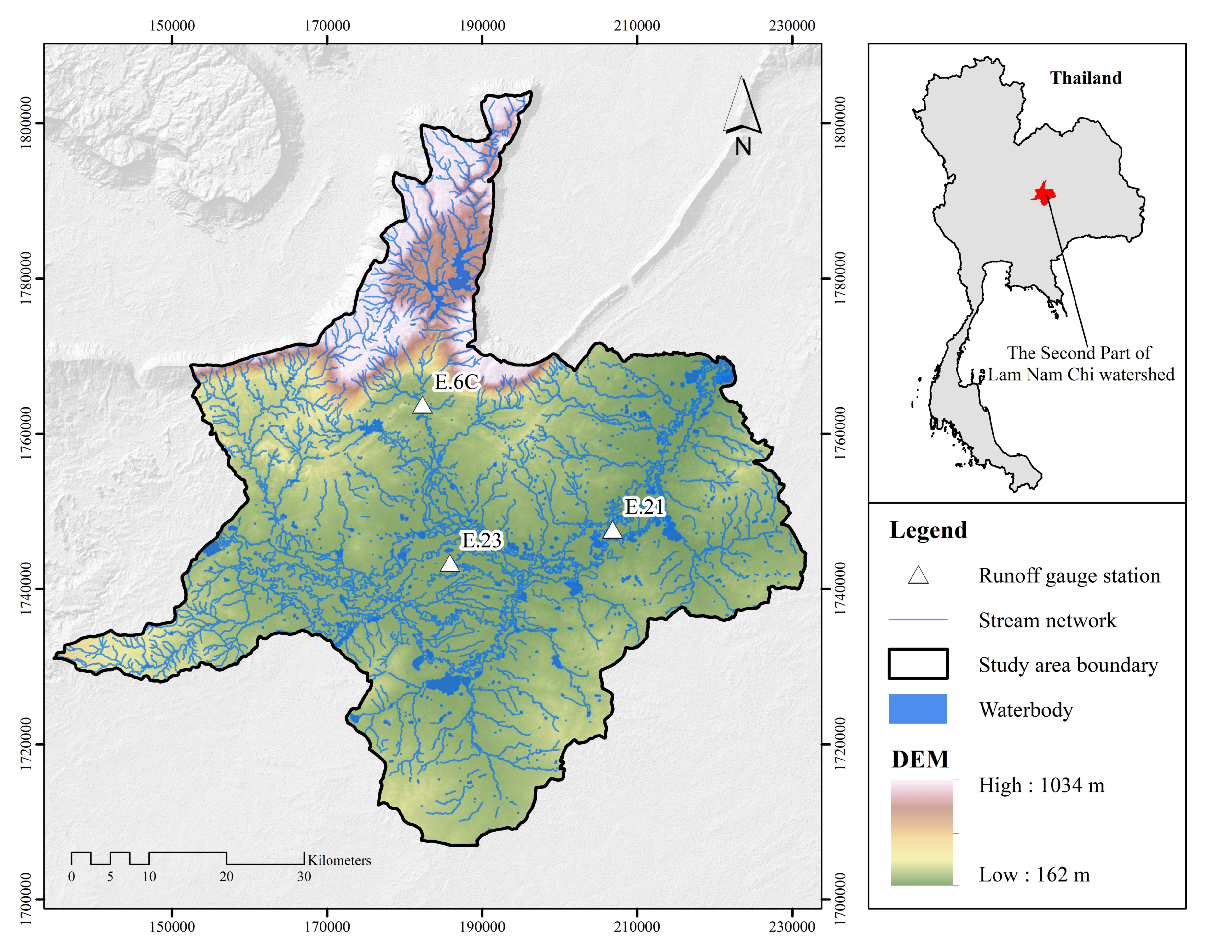
Figure 1.
Terrain characteristics of the study area with runoff gauge stations.
Figure 1.
Terrain characteristics of the study area with runoff gauge stations.
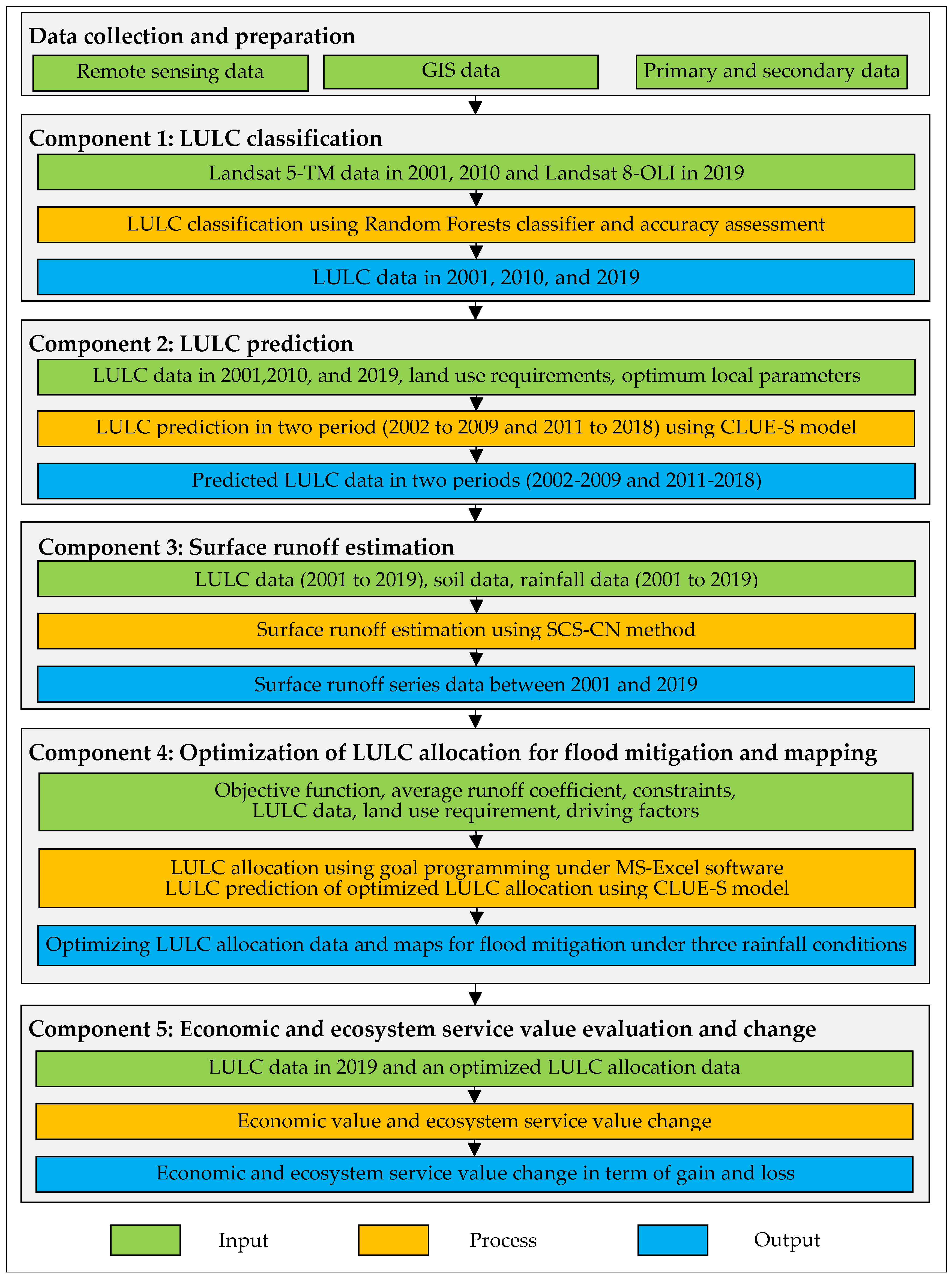
Figure 2.
Workflow of the research methodology.
Figure 2.
Workflow of the research methodology.
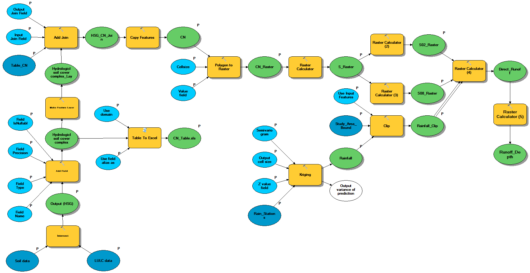
Figure 3.
Schematic diagram of Model Builder for surface runoff estimation.
Figure 3.
Schematic diagram of Model Builder for surface runoff estimation.
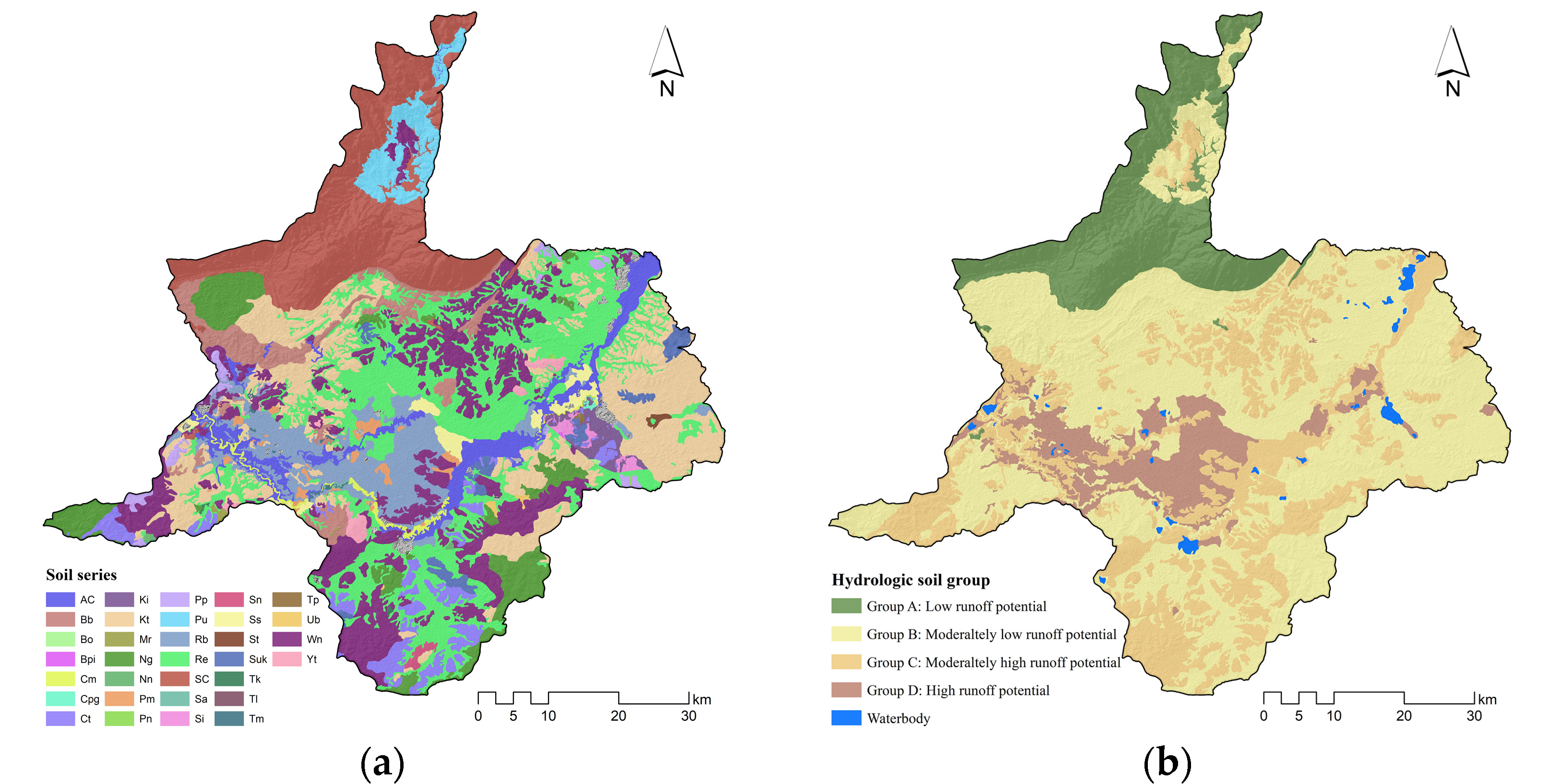
Figure 4.
Spatial distribution of (a) soil series and (b) hydrologic soil group.
Figure 4.
Spatial distribution of (a) soil series and (b) hydrologic soil group.
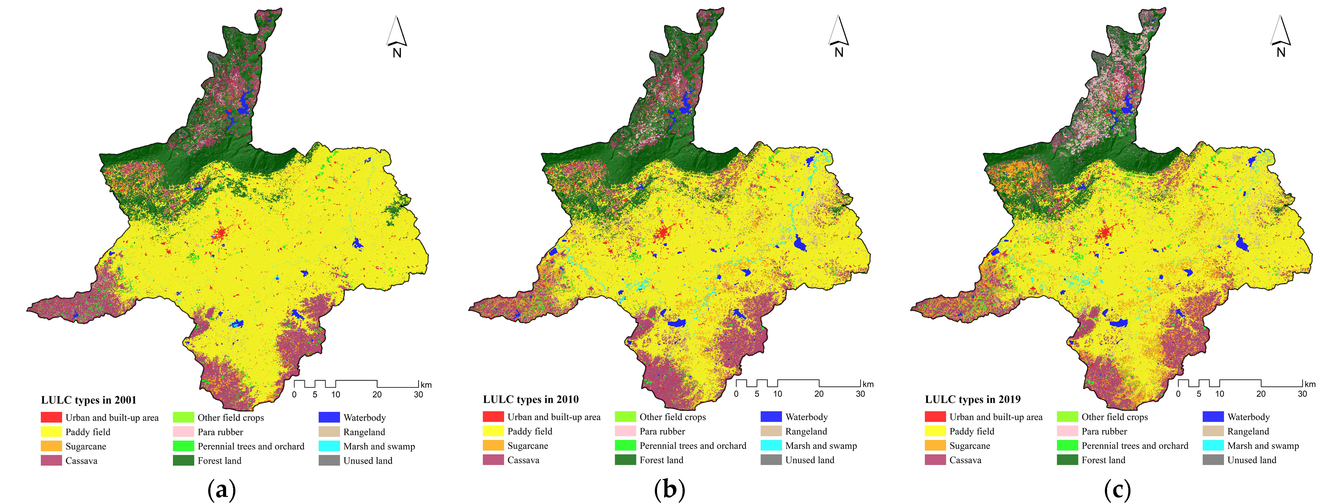
Figure 5.
Spatial distribution of the LULC classification in: (a) 2001, (b) 2010, and (c) 2019.
Figure 5.
Spatial distribution of the LULC classification in: (a) 2001, (b) 2010, and (c) 2019.
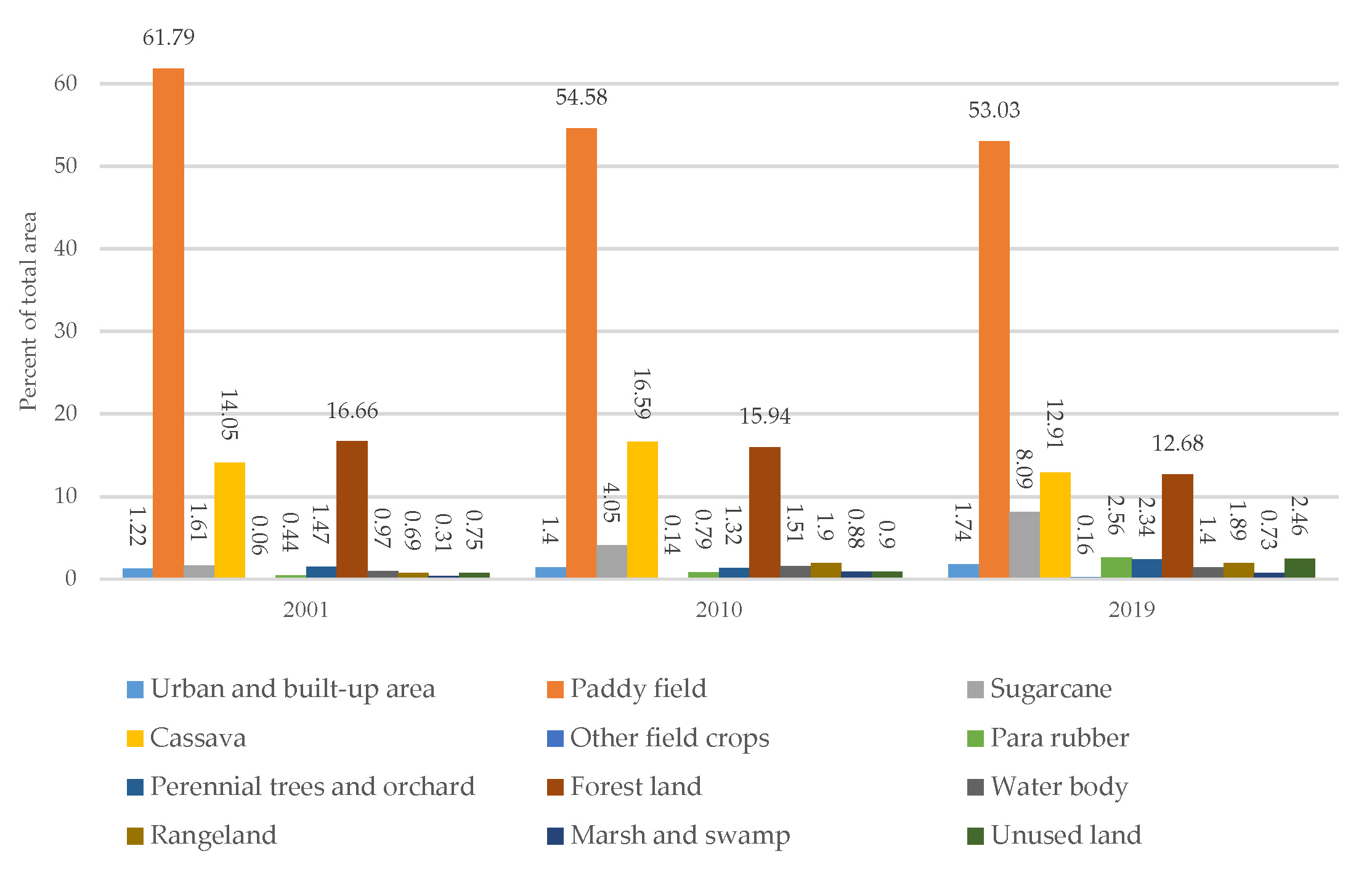
Figure 6.
Multitemporal change of LULC type coverage in 2001, 2010, and 2019.
Figure 6.
Multitemporal change of LULC type coverage in 2001, 2010, and 2019.
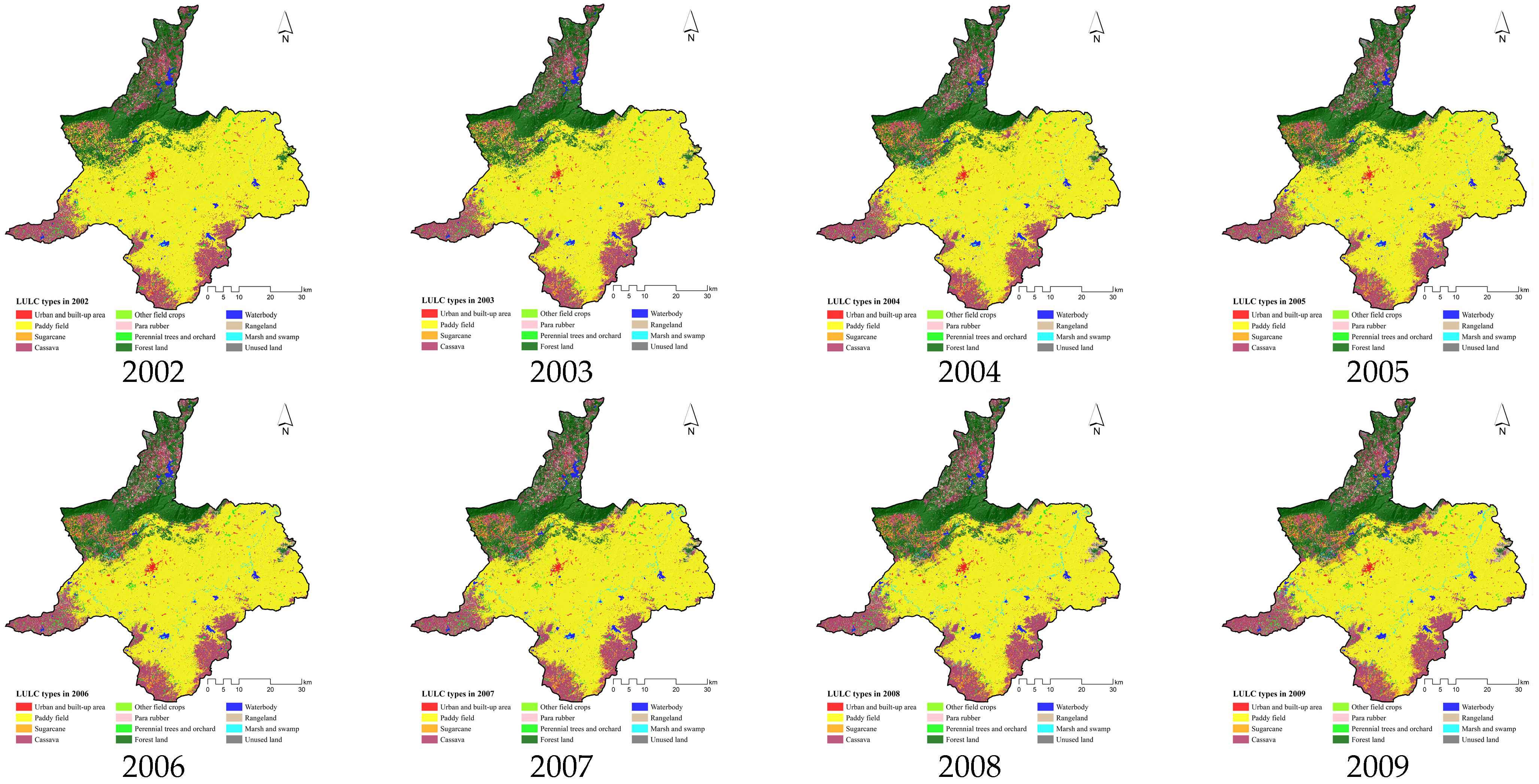
Figure 7.
Spatial distribution of predicted LULC data between 2002 and 2009.
Figure 7.
Spatial distribution of predicted LULC data between 2002 and 2009.
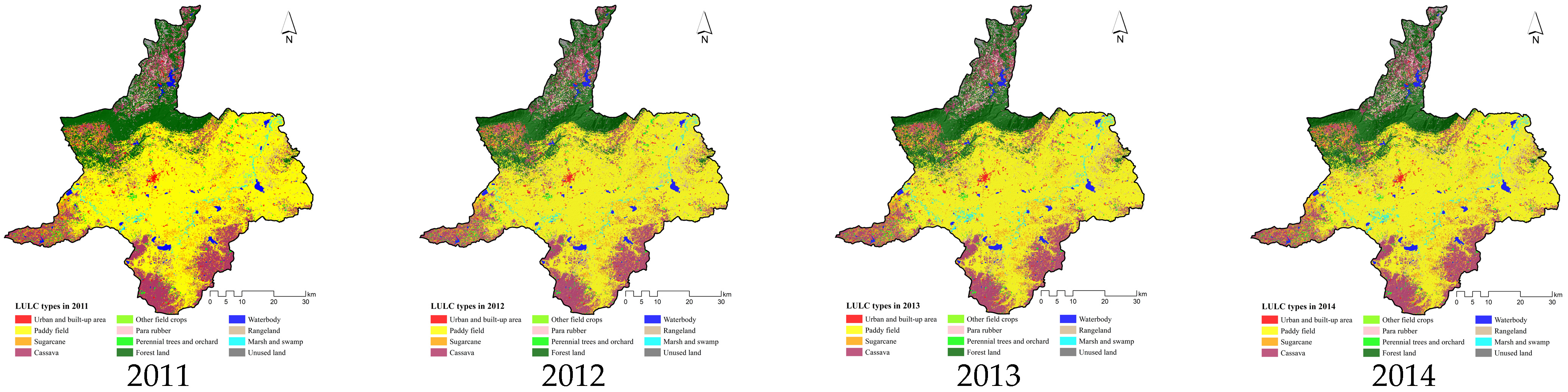
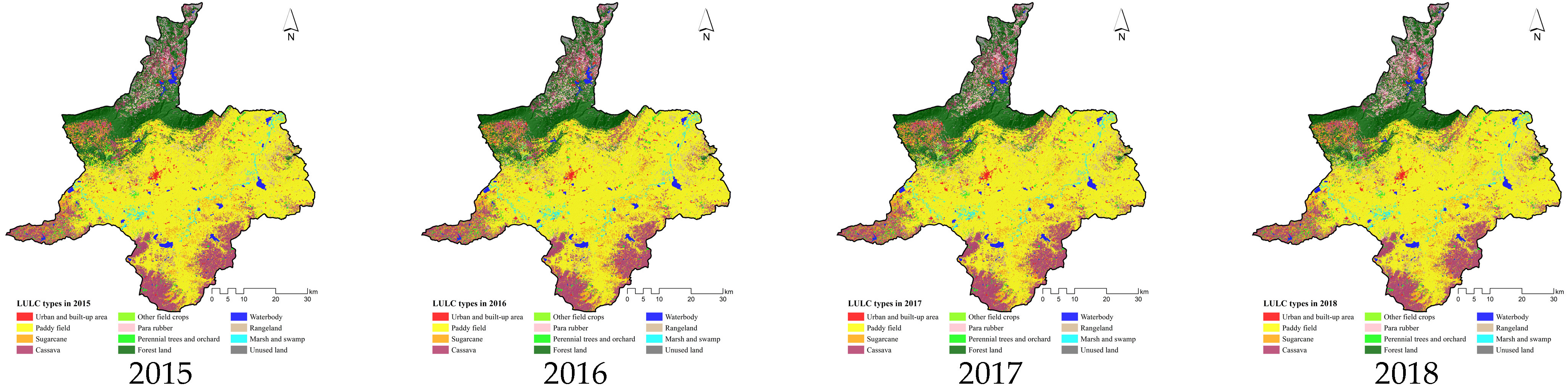
Figure 8.
Spatial distribution of the predicted LULC data between 2011 and 2018.
Figure 8.
Spatial distribution of the predicted LULC data between 2011 and 2018.
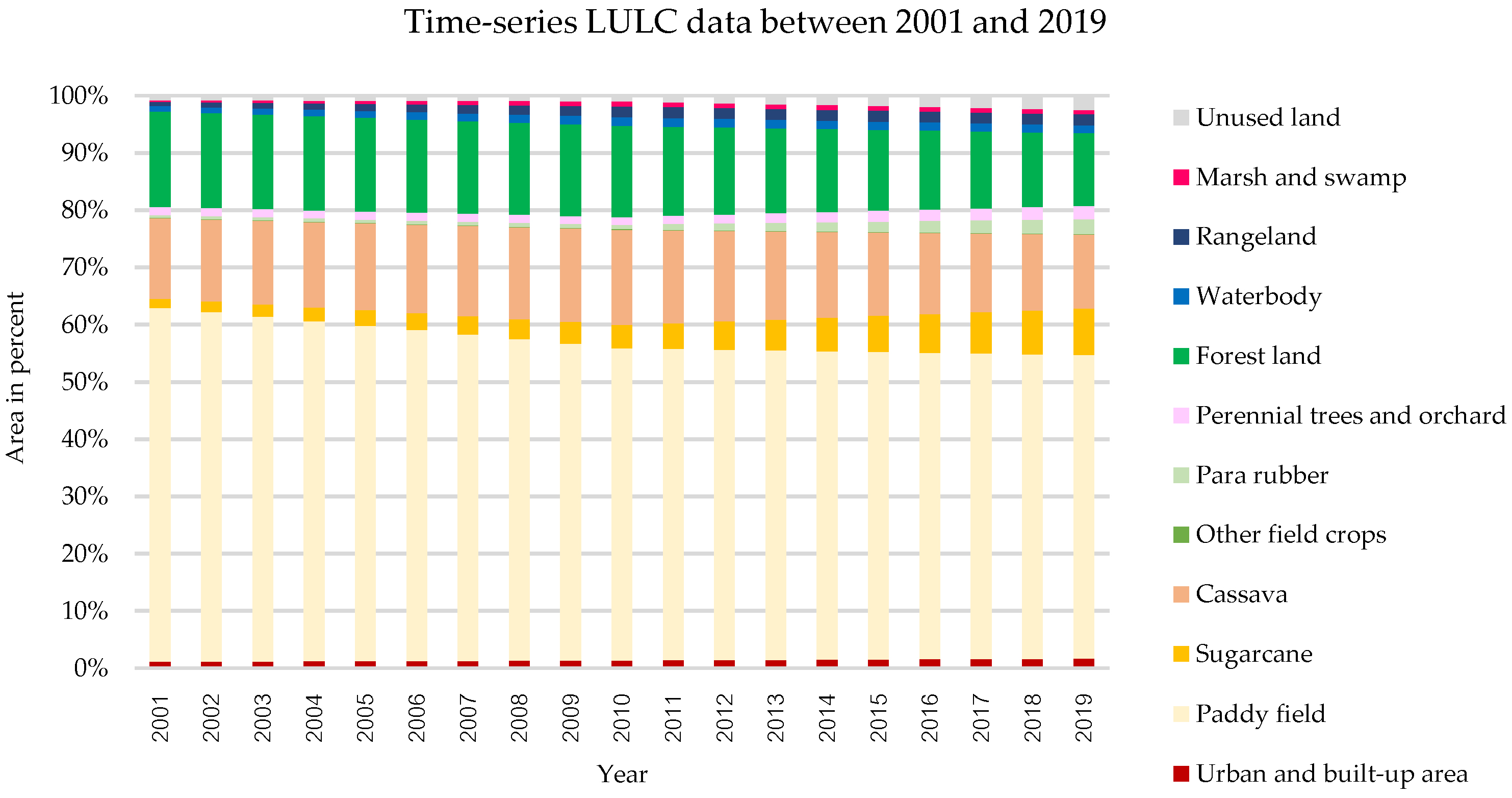
Figure 9.
Proportion area of LULC type of LULC data between 2001 and 2019.
Figure 9.
Proportion area of LULC type of LULC data between 2001 and 2019.
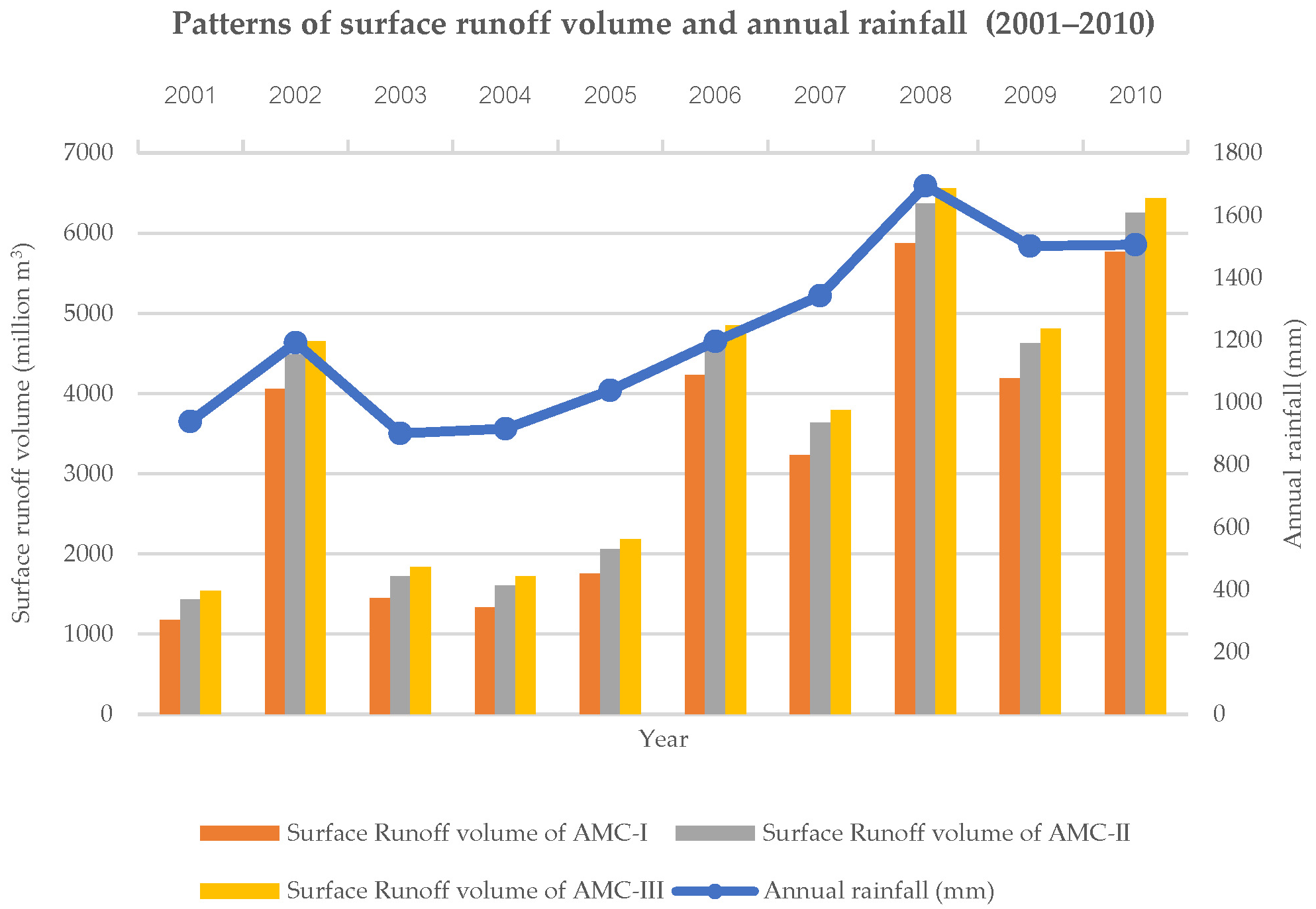
Figure 10.
Patterns of surface runoff volume of the three AMC conditions and annual rainfall data between 2001 and 2010.
Figure 10.
Patterns of surface runoff volume of the three AMC conditions and annual rainfall data between 2001 and 2010.
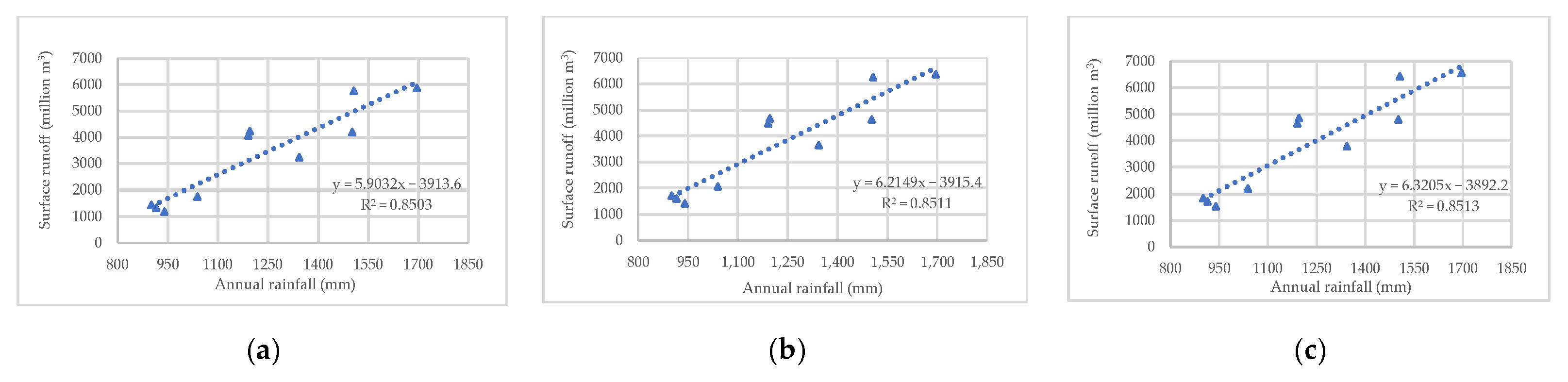
Figure 11.
Relationship between surface runoff volume and annual rainfall: (a) AMC-I, (b) AMC-II, and (c) AMC-III.
Figure 11.
Relationship between surface runoff volume and annual rainfall: (a) AMC-I, (b) AMC-II, and (c) AMC-III.
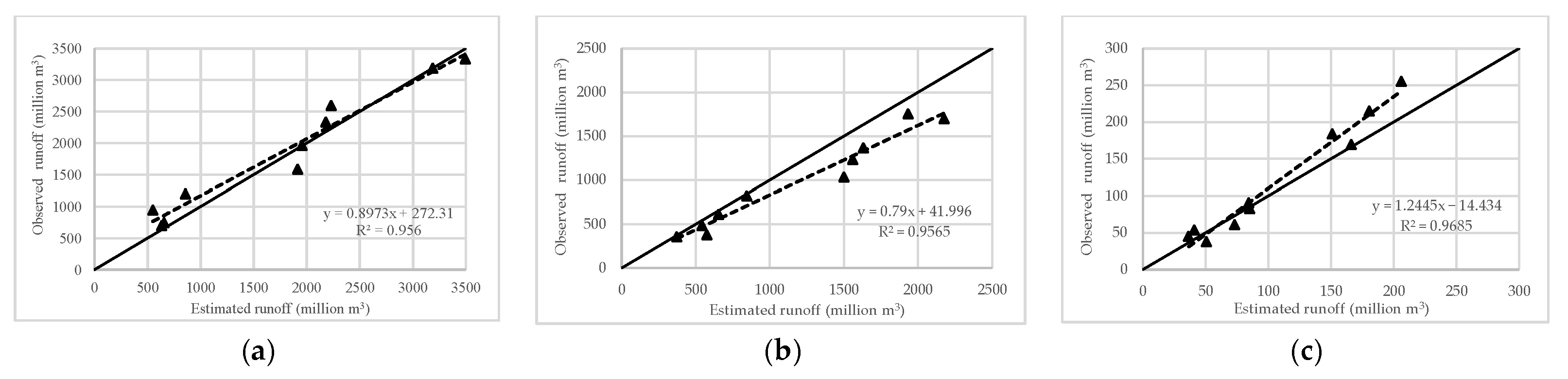
Figure 12.
Relationship between the observed and estimated runoff between 2001 and 2010 under the AMC-I condition at the three stations: (a) E.21 station, (b) E.23 station, and (c) E.6C station.
Figure 12.
Relationship between the observed and estimated runoff between 2001 and 2010 under the AMC-I condition at the three stations: (a) E.21 station, (b) E.23 station, and (c) E.6C station.
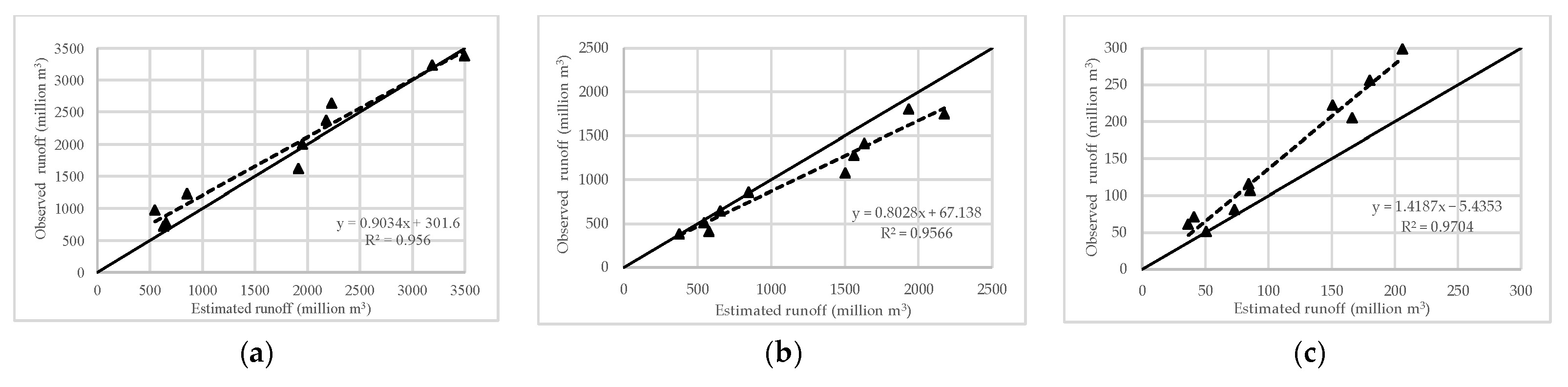
Figure 13.
Relationship between the observed and estimated runoff between 2001 and 2010 under the AMC-II condition at the three stations: (a) E.21 station, (b) E.23 station, and (c) E.6C station.
Figure 13.
Relationship between the observed and estimated runoff between 2001 and 2010 under the AMC-II condition at the three stations: (a) E.21 station, (b) E.23 station, and (c) E.6C station.
Figure 14.
Relationship between the observed and estimated runoff between 2001 and 2010 under the AMC-III condition at the three stations: (a) E.21 station, (b) E.23 station, and (c) E.6C station.
Figure 14.
Relationship between the observed and estimated runoff between 2001 and 2010 under the AMC-III condition at the three stations: (a) E.21 station, (b) E.23 station, and (c) E.6C station.
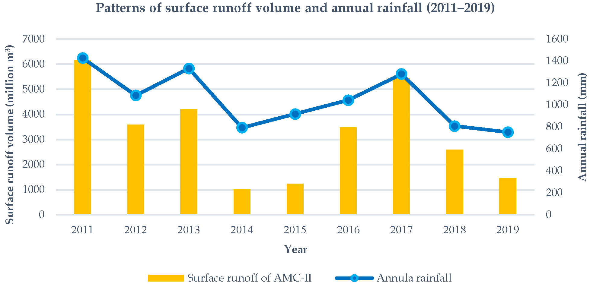
Figure 15.
Pattern of surface runoff volume and annual rainfall of AMC-II between 2011 and 2019.
Figure 15.
Pattern of surface runoff volume and annual rainfall of AMC-II between 2011 and 2019.
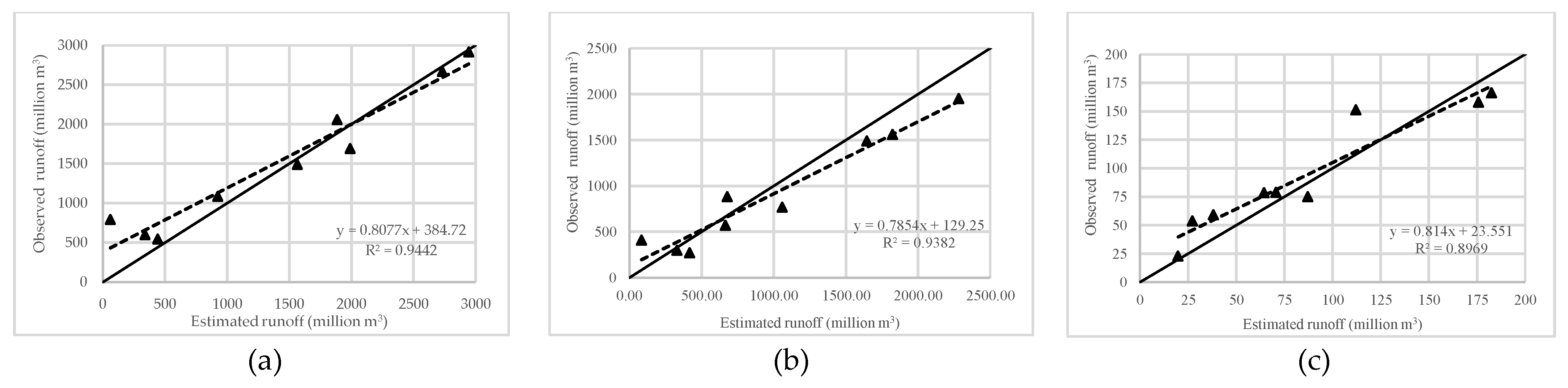
Figure 16.
Relationship between the observed and estimated runoff between 2011 and 2019 at the three stations: (a) E.21 station, (b) E.23 station, and (c) E.6C station.
Figure 16.
Relationship between the observed and estimated runoff between 2011 and 2019 at the three stations: (a) E.21 station, (b) E.23 station, and (c) E.6C station.
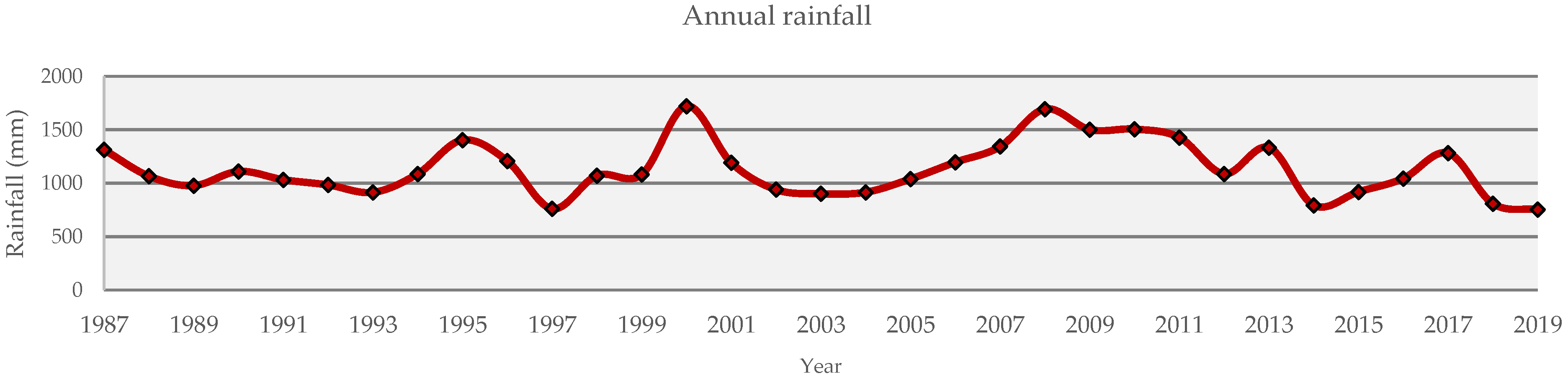
Figure 17.
Annual rainfall of Chaiyaphum meteorological station (1987–2019).
Figure 17.
Annual rainfall of Chaiyaphum meteorological station (1987–2019).
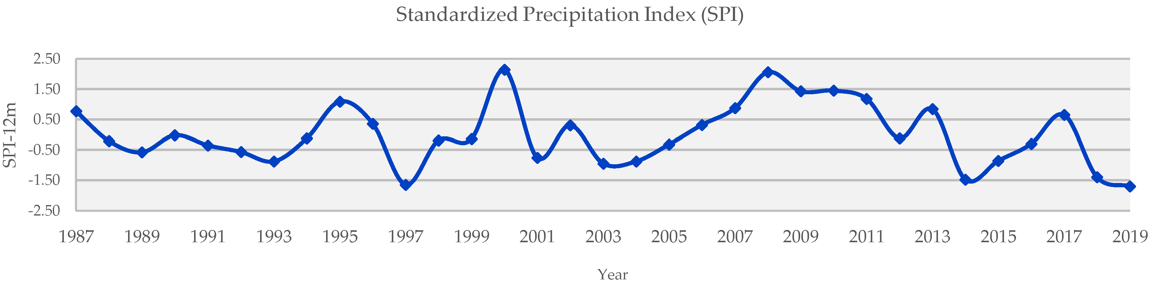
Figure 18.
The 12-month SPI values of Chaiyaphum meteorological station (1987 and 2019).
Figure 18.
The 12-month SPI values of Chaiyaphum meteorological station (1987 and 2019).
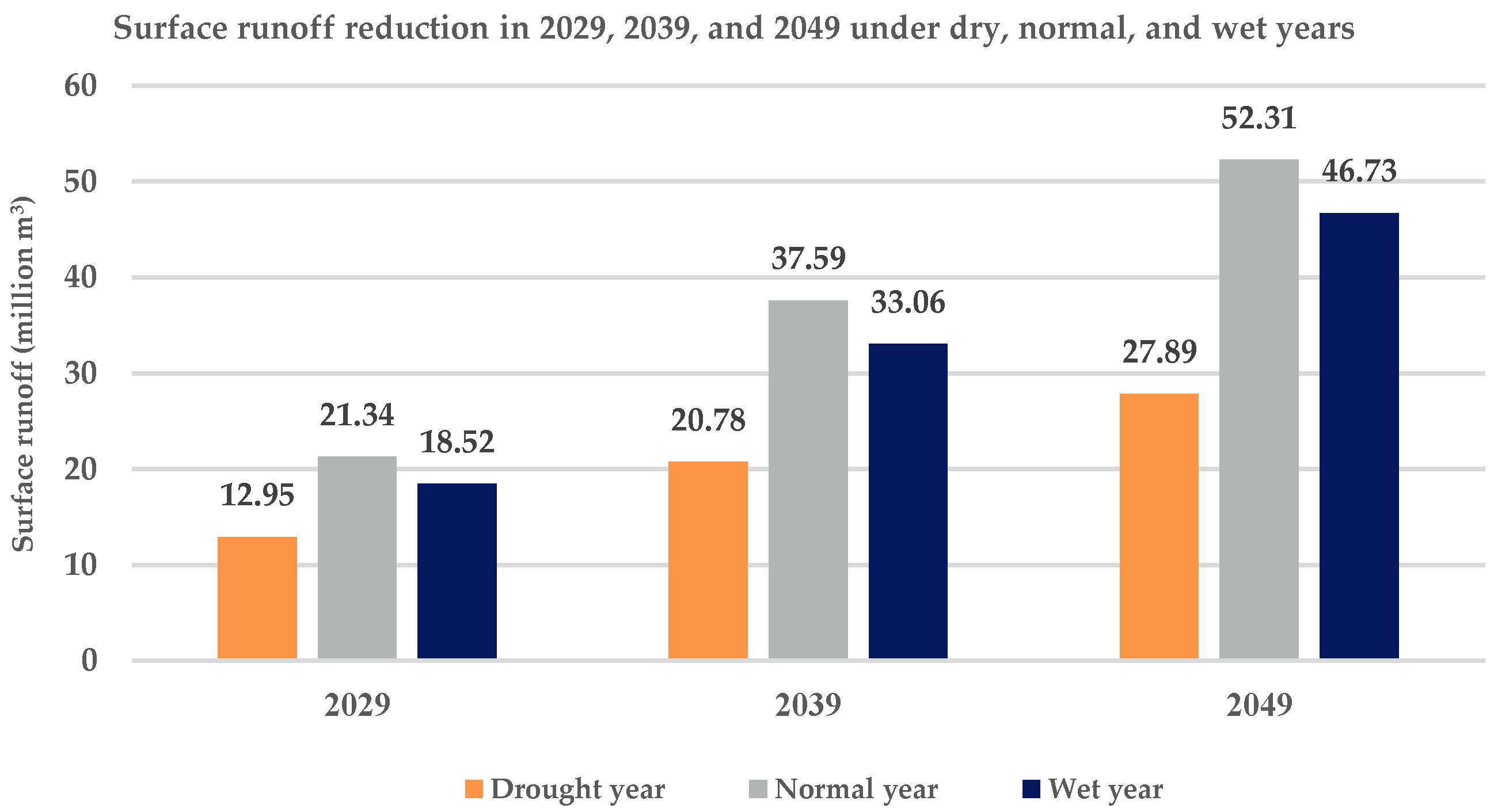
Figure 19.
Surface runoff reduction in 2029, 2039, and 2049 in dry, normal, and wet years.
Figure 19.
Surface runoff reduction in 2029, 2039, and 2049 in dry, normal, and wet years.
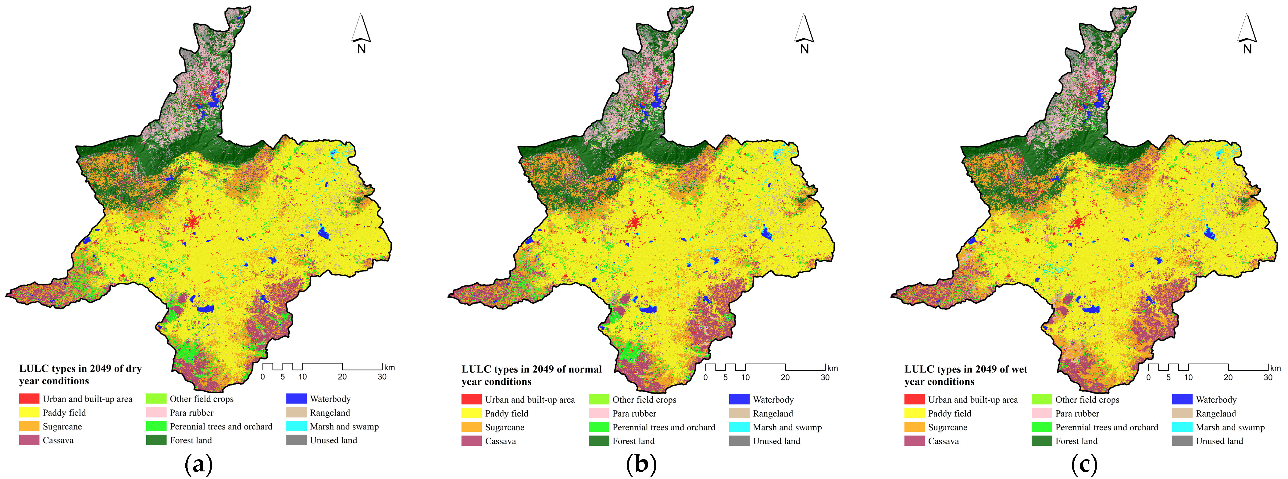
Figure 20.
Spatial distribution of predicted LULC data in 2049: (a) Dry years, (b) normal years, and (c) wet years.
Figure 20.
Spatial distribution of predicted LULC data in 2049: (a) Dry years, (b) normal years, and (c) wet years.
Figure 21.
Spatial distribution of economic value in 2049: (a) Actual LULC 2019, (b) dry years, (c) normal years, and (d) wet years.
Figure 21.
Spatial distribution of economic value in 2049: (a) Actual LULC 2019, (b) dry years, (c) normal years, and (d) wet years.
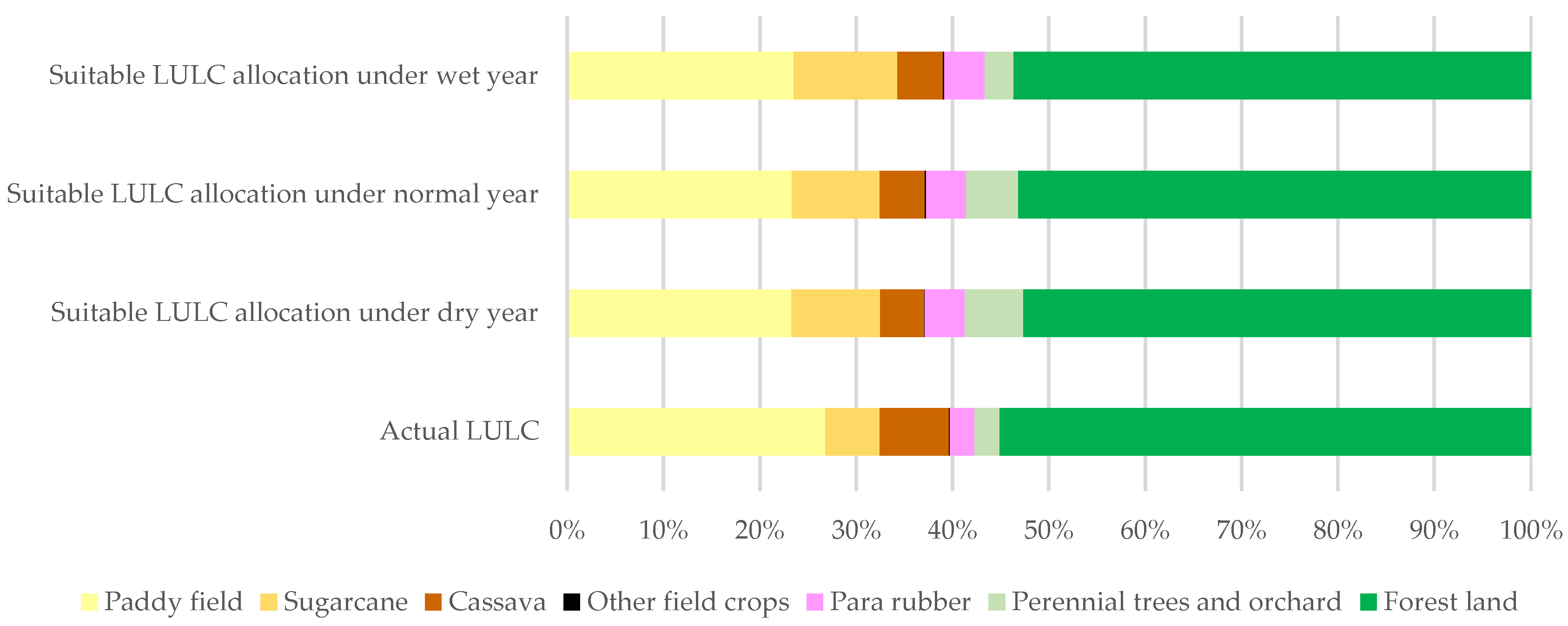
Figure 22.
Contribution of the future economic value of LULC type of actual LULC and suitable LULC allocation for flood mitigation (dry, normal, and wet years).
Figure 22.
Contribution of the future economic value of LULC type of actual LULC and suitable LULC allocation for flood mitigation (dry, normal, and wet years).
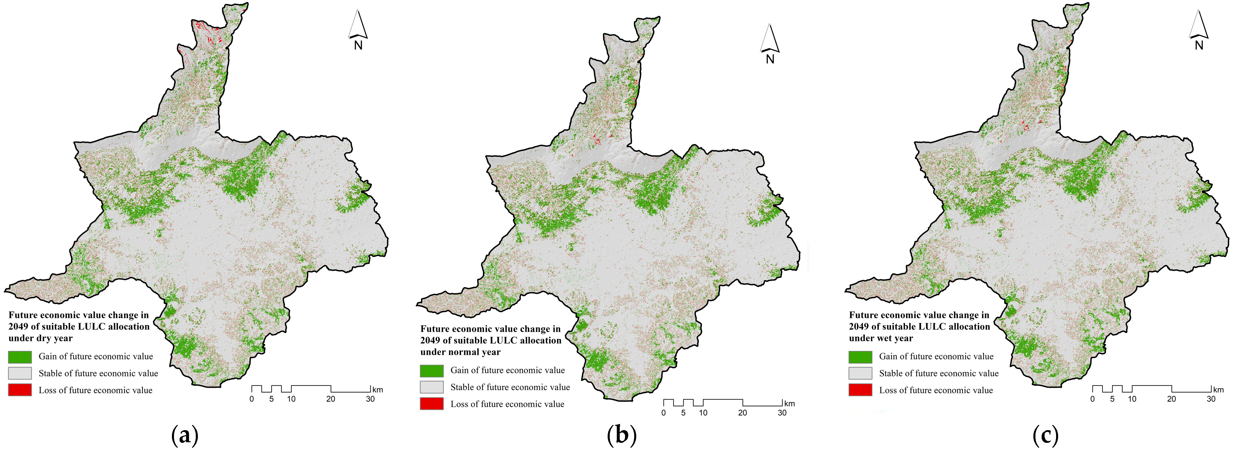
Figure 23.
Gain and loss of future economic value of suitable LULC allocation for flood mitigation in 2049: (a) Dry years, (b) normal years, and (c) wet years.
Figure 23.
Gain and loss of future economic value of suitable LULC allocation for flood mitigation in 2049: (a) Dry years, (b) normal years, and (c) wet years.
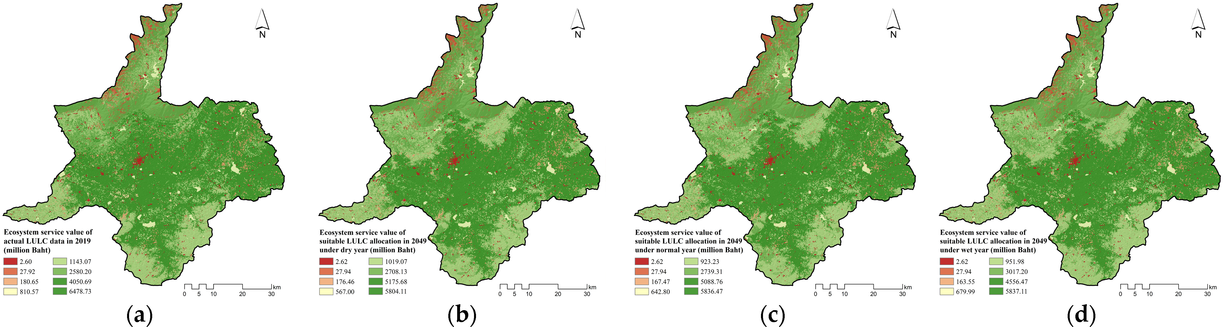
Figure 24.
Spatial distribution of the ecosystem service value: (a) Actual LULC 2019, (b) dry years, (c) normal years, and (d) wet years.
Figure 24.
Spatial distribution of the ecosystem service value: (a) Actual LULC 2019, (b) dry years, (c) normal years, and (d) wet years.
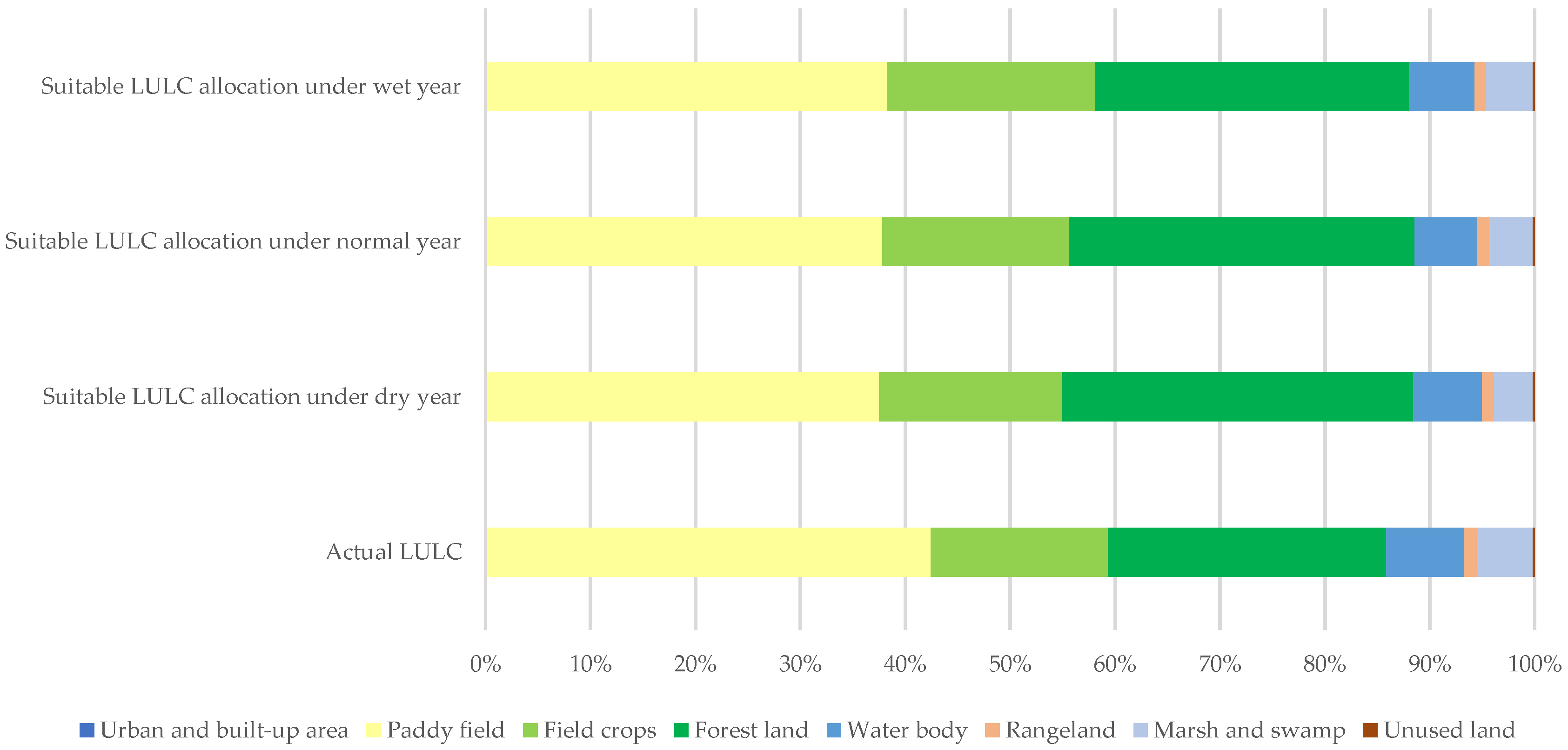
Figure 25.
Contribution of the ecosystem service value of each LULC type of actual LULC and suitable LULC allocation for flood mitigation (dry, normal, and wet years).
Figure 25.
Contribution of the ecosystem service value of each LULC type of actual LULC and suitable LULC allocation for flood mitigation (dry, normal, and wet years).
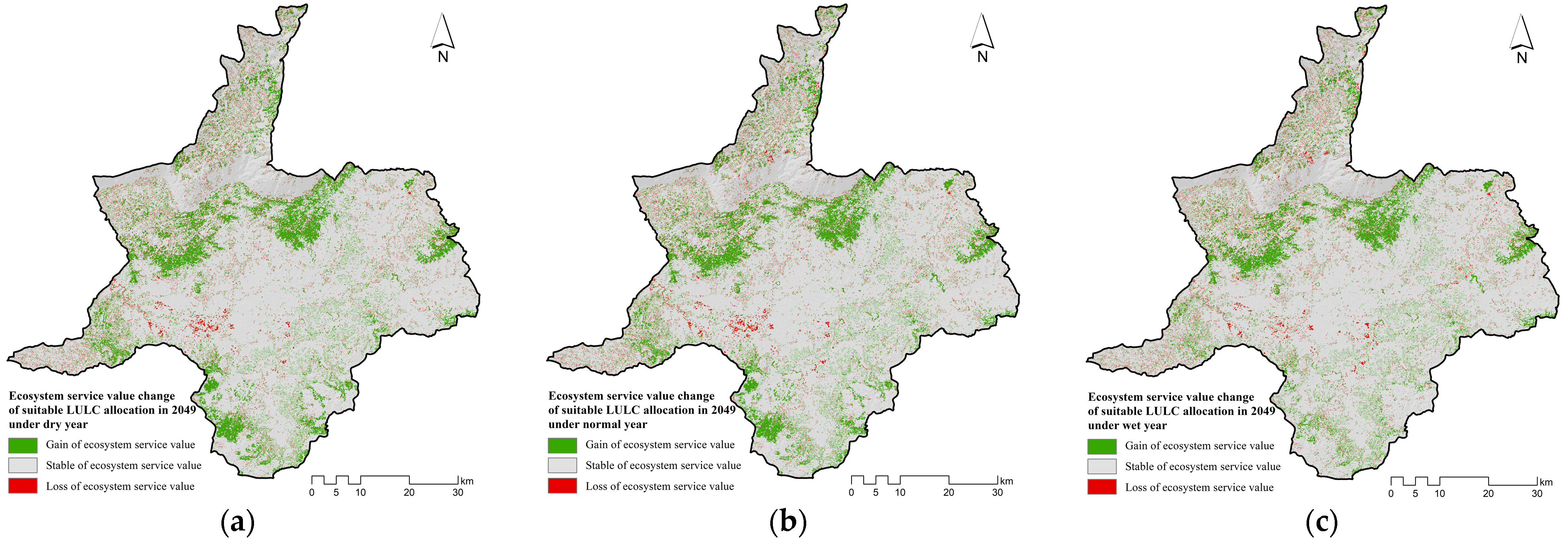
Figure 26.
Gain and loss of ESV of suitable LULC allocation for flood mitigation in 2049: (a) Dry years, (b) normal years, and (c) wet years.
Figure 26.
Gain and loss of ESV of suitable LULC allocation for flood mitigation in 2049: (a) Dry years, (b) normal years, and (c) wet years.
Table 1.
List of data collection and preparation for data analysis in this study.
Table 1.
List of data collection and preparation for data analysis in this study.
| Data | Data Collection | Data Preparation | Source |
|---|
| Primary | Ground reference | - | - |
| Secondary | Runoff | - | RID |
| Annual rainfall | Interpolation | TMD |
| Socioeconomic data | Population density | DOPA |
| Income per capita | NESDC |
| Remote Sensing | Landsat 5 TM: Path 128 Row 49, 6 January 2001
Landsat 5 TM: Path 129 Row 49, 14 February 2001
Landsat 5 TM: Path 128 Row 49, 16 February 2010
Landsat 5 TM: Path 129 Row 49, 23 February 2010
Landsat 8 OLI: Path 128 Row 49, 24 January 2019
Landsat 8 OLI: Path 129 Row 49, 31 January 2019 | - | USGS |
| Satellite image from Google Earth in 2010 | - | Google |
| Color orthophotograph | - | RTSD |
| GIS | Administrative boundary | - | DEQP |
| Soil (soil series) | Recode | LDD |
| Watershed boundary | - | RID |
| Elevation | Extract from DEM | SRTM |
| Slope | Extract from DEM | SRTM |
| Road network | Buffering | MOT, DEQP |
| Stream | Buffering | RTSD |
| Urban area | Buffering | LULC data |
Table 2.
Runoff curve number under AMC-I, -II, and -III.
Table 2.
Runoff curve number under AMC-I, -II, and -III.
| LULC Types | CN Value of AMC-I | CN Value of AMC-II | CN Value of AMC-III |
|---|
| A | B | C | D | A | B | C | D | A | B | C | D |
|---|
| Urban and built-up area | 77.26 | 82.85 | 86.81 | 88.86 | 89 | 92 | 94 | 95 | 94.9 | 96.36 | 97.3 | 97.76 |
| Cassava and other field crops | 51.92 | 64.16 | 75.49 | 80.94 | 72 | 81 | 88 | 91 | 85.54 | 90.75 | 94.4 | 95.88 |
| Sugarcane | 28.75 | 48.32 | 61.24 | 68.8 | 49 | 69 | 79 | 84 | 68.85 | 83.66 | 89.64 | 92.35 |
| Paddy fields | 43.82 | 57.08 | 68.8 | 75.49 | 65 | 76 | 84 | 88 | 81.03 | 87.93 | 92.35 | 94.4 |
| Rangeland | 28.75 | 48.32 | 61.24 | 68.8 | 49 | 69 | 79 | 84 | 68.85 | 83.66 | 89.64 | 92.35 |
| Para rubber and perennial trees and orchards | 24.06 | 43.82 | 57.08 | 65.68 | 43 | 65 | 76 | 82 | 63.44 | 81.03 | 87.93 | 91.29 |
| Forest land | 15.25 | 33.92 | 49.49 | 58.44 | 30 | 55 | 70 | 77 | 49.64 | 73.76 | 84.29 | 88.51 |
| Waterbodies and marshes and swamps | 95.37 | 95.37 | 95.37 | 95.37 | 98 | 98 | 98 | 98 | 99.12 | 99.12 | 99.12 | 99.12 |
| Unused land | 58.44 | 72.07 | 80.94 | 86.81 | 77 | 86 | 91 | 94 | 88.51 | 93.39 | 95.88 | 97.3 |
Table 3.
Model performance scale.
Table 3.
Model performance scale.
| Statistics Measurement | Performance Ratings |
|---|
| Unsatisfactory | Satisfactory | Good | Very Good |
|---|
| NSE | <0.5 | 0.5–0.65 | 0.65–0.75 | 0.75–1 |
| R2 | <0.5 | 0.5–0.6 | 0.6–0.7 | 0.7–1 |
| PBIAS | >25 | 15–25 | 10–15 | <10 |
Table 4.
LULC type and coefficient value for ESV evaluation.
Table 4.
LULC type and coefficient value for ESV evaluation.
| No. | LULC Classification for RF | LULC Classification for ESV 1 | Coefficient Values (USD/ha/year) 1 |
|---|
| 1 | Urban and built-up areas | Construction land | 12.7 |
| 2 | Paddy fields | Cultivated land | 1032.3 |
| 3 | Field crops | Cultivated land | 1032.3 |
| 4 | Para rubber | Forest land | 1949.0 |
| 5 | Perennial trees and orchards | Forest land | 1949.0 |
| 6 | Forest land | Forest land | 1949.0 |
| 7 | Waterbodies | Waterbodies | 6873.7 |
| 8 | Rangeland | Rangeland | 808.6 |
| 9 | Wetland | Wetland | 9368.7 |
| 10 | Miscellaneous land | Unused land | 96.3 |
Table 5.
Area and percentage of LULC data in 2001, 2010, and 2019.
Table 5.
Area and percentage of LULC data in 2001, 2010, and 2019.
| No. | LULC Type | LULC 2001 | LULC 2010 | LULC 2019 |
|---|
| Area (km2) | Percentage | Area (km2) | Percentage | Area (km2) | Percentage |
|---|
| 1 | Urban and built-up areas | 46.17 | 1.22 | 53.21 | 1.4 | 65.84 | 1.74 |
| 2 | Paddy fields | 2344.39 | 61.79 | 2070.71 | 54.58 | 2012.16 | 53.03 |
| 3 | Sugarcane | 61.25 | 1.61 | 153.52 | 4.05 | 306.85 | 8.09 |
| 4 | Cassava | 532.95 | 14.05 | 629.33 | 16.59 | 489.91 | 12.91 |
| 5 | Other field crops | 2.09 | 0.06 | 5.19 | 0.14 | 6.19 | 0.16 |
| 6 | Para rubber | 16.56 | 0.44 | 30.05 | 0.79 | 97.03 | 2.56 |
| 7 | Perennial trees and orchards | 55.76 | 1.47 | 50.21 | 1.32 | 88.95 | 2.34 |
| 8 | Forest land | 632 | 16.66 | 604.7 | 15.94 | 481.3 | 12.68 |
| 9 | Waterbodies | 36.81 | 0.97 | 57.46 | 1.51 | 53.3 | 1.4 |
| 10 | Rangeland | 26.03 | 0.69 | 72.11 | 1.9 | 71.65 | 1.89 |
| 11 | Marshes and swamps | 11.64 | 0.31 | 33.4 | 0.88 | 27.73 | 0.73 |
| 12 | Unused land | 28.57 | 0.75 | 34.33 | 0.9 | 93.32 | 2.46 |
| Total | 3794.22 | 100.00 | 3794.22 | 100.00 | 3794.22 | 100.00 |
Table 6.
Simple LULC change detection between 2001 and 2010.
Table 6.
Simple LULC change detection between 2001 and 2010.
| LULC | LULC Type (Area, km2) |
|---|
| UR | PA | SU | CA | PC | PR | PO | FO | WA | RA | MA | UL |
|---|
| In 2001 | 46.17 | 2344.39 | 61.25 | 532.95 | 2.09 | 16.56 | 55.76 | 632.00 | 36.81 | 26.03 | 11.64 | 28.57 |
| In 2010 | 53.21 | 2070.71 | 153.52 | 629.33 | 5.19 | 30.05 | 50.21 | 604.70 | 57.46 | 72.11 | 33.40 | 34.33 |
| Change area | 7.04 | –273.68 | 92.27 | 96.38 | 3.11 | 13.49 | –5.54 | –27.30 | 20.65 | 46.08 | 21.76 | 5.76 |
| Annual change rate | 0.78 | –30.41 | 10.25 | 10.71 | 0.35 | 1.50 | –0.62 | –3.03 | 2.29 | 5.12 | 2.42 | 0.64 |
| Percentage of change | 0.19 | –7.21 | 2.43 | 2.54 | 0.08 | 0.36 | –0.15 | –0.72 | 0.54 | 1.21 | 0.57 | 0.15 |
Table 7.
Simple LULC change detection between 2010 and 2019.
Table 7.
Simple LULC change detection between 2010 and 2019.
| LULC | LULC Type (Area, km2) |
|---|
| UR | PA | SU | CA | PC | PR | PO | FO | WA | RA | MA | UL |
|---|
| In 2010 | 53.21 | 2070.71 | 153.52 | 629.33 | 5.19 | 30.05 | 50.21 | 604.70 | 57.46 | 72.11 | 33.40 | 34.33 |
| In 2019 | 65.84 | 2012.16 | 306.85 | 489.91 | 6.19 | 97.03 | 88.95 | 481.30 | 53.30 | 71.65 | 27.73 | 93.32 |
| Change area | 12.63 | –58.55 | 153.33 | –139.41 | 1.00 | 66.99 | 38.73 | –123.41 | –4.16 | –0.47 | –5.67 | 58.99 |
| Annual change rate | 1.40 | –6.51 | 17.04 | –15.49 | 0.11 | 7.44 | 4.30 | –13.71 | –0.46 | –0.05 | –0.63 | 6.55 |
| Percentage of change | 0.33 | –1.54 | 4.04 | –3.67 | 0.03 | 1.77 | 1.02 | –3.25 | –0.11 | –0.01 | –0.15 | 1.55 |
Table 8.
Simple LULC change detection between 2001 and 2019.
Table 8.
Simple LULC change detection between 2001 and 2019.
| LULC | LULC Type (Area, km2) |
|---|
| UR | PA | SU | CA | PC | PR | PO | FO | WA | RA | MA | UL |
|---|
| In 2001 | 46.17 | 2344.39 | 61.25 | 532.95 | 2.09 | 16.56 | 55.76 | 632 | 36.81 | 26.03 | 11.64 | 28.57 |
| In 2019 | 65.84 | 2012.16 | 306.85 | 489.91 | 6.19 | 97.03 | 88.95 | 481.3 | 53.3 | 71.65 | 27.73 | 93.32 |
| Change area | 19.67 | –332.23 | 245.6 | –43.04 | 4.1 | 80.47 | 33.19 | –150.7 | 16.49 | 45.62 | 16.09 | 64.75 |
| Annual change rate | 1.09 | –18.46 | 13.64 | –2.39 | 0.23 | 4.47 | 1.84 | –8.37 | 0.92 | 2.53 | 0.89 | 3.60 |
| Percentage of change | 0.52 | –8.76 | 6.47 | –1.13 | 0.11 | 2.12 | 0.87 | –3.97 | 0.43 | 1.20 | 0.42 | 1.71 |
Table 9.
Multiple linear equations of each LULC type location preference and area under the curve value from logistic regression analysis.
Table 9.
Multiple linear equations of each LULC type location preference and area under the curve value from logistic regression analysis.
| Driving Factors | LULC Type |
|---|
| UR | PD | SU | CA | FC | PR | OP | FO | WA | RA | MA | UL |
|---|
| Constant | 0.0930 | 10.8831 | 94.6560 | –38.4766 | 207.9784 | 24.1870 | –38.4831 | 87.3484 | –4.6862 | –80.0118 | 5.0436 | –8.6344 |
| X1 | n. s. | –0.0947 | –0.0001 | 0.0042 | 0.0101 | 0.0083 | n. s. | 0.0032 | 0.0068 | –0.0043 | –0.0467 | 0.0093 |
| X2 | n. s. | n. s. | –0.1943 | –0.1030 | –0.2144 | –0.0730 | –0.1314 | 0.1886 | –0.6715 | n. s. | n. s. | –0.0290 |
| X3 | n. s. | 0.0130 | –0.1264 | 0.0477 | –0.2850 | –0.0398 | 0.0454 | –0.1167 | n. s. | 0.0991 | n. s. | n. s. |
| X4 | n. s. | n. s. | n. s. | n. s. | n. s. | n. s. | n. s. | n. s. | n. s. | n. s. | n. s. | n. s. |
| X5 | 0.0008 | –0.0018 | –0.0117 | –0.0148 | n. s. | –0.0186 | –0.0043 | –0.0113 | n. s. | –0.0060 | –0.0059 | n. s. |
| X6 | –0.0064 | n. s. | n. s. | n. s. | n. s. | n. s. | n. s. | n. s. | 0.0014 | n. s. | n. s. | n. s. |
| X7 | n. s. | n. s. | n. s. | 0.0010 | n. s. | –0.0014 | n. s. | n. s. | –0.0037 | n. s. | –0.0053 | n. s. |
| X8 | –0.0182 | n. s. | n. s. | n. s. | n. s. | n. s. | n. s. | n. s. | n. s. | n. s. | n. s. | n. s. |
| AUC | 0.9824 | 0.9763 | 0.7677 | 0.7942 | 0.9355 | 0.9440 | 0.6186 | 0.9289 | 0.8318 | 0.7445 | 0.8628 | 0.8693 |
Table 10.
Conversion matrix of possible changes between 2010 and 2019.
Table 10.
Conversion matrix of possible changes between 2010 and 2019.
| | LULC Types | LULC Type Possible Change in 2019 |
|---|
| UR | PA | SU | CA | FC | PR | PO | FO | WA | RA | MA | UL |
|---|
| LULC in 2010 | Urban and built-up areas (UR) | 1 | 0 | 0 | 0 | 0 | 0 | 0 | 0 | 0 | 0 | 0 | 0 |
| Paddy fields (PA) | 0 | 1 | 1 | 1 | 0 | 0 | 1 | 0 | 0 | 1 | 1 | 0 |
| Sugarcane (SU) | 1 | 1 | 1 | 1 | 0 | 0 | 1 | 0 | 0 | 0 | 0 | 0 |
| Cassava (CA) | 1 | 1 | 1 | 1 | 0 | 1 | 1 | 0 | 0 | 1 | 0 | 1 |
| Other field crops (FC) | 0 | 0 | 1 | 1 | 1 | 0 | 0 | 0 | 0 | 0 | 0 | 0 |
| Para rubber (PR) | 0 | 0 | 0 | 1 | 1 | 1 | 0 | 0 | 0 | 0 | 0 | 1 |
| Perennial trees and orchards (PO) | 0 | 0 | 1 | 0 | 0 | 0 | 1 | 0 | 0 | 0 | 0 | 0 |
| Forest land (FO) | 1 | 0 | 0 | 0 | 0 | 1 | 1 | 1 | 0 | 1 | 0 | 1 |
| Waterbodies (WA) | 1 | 0 | 1 | 0 | 0 | 0 | 0 | 0 | 1 | 0 | 1 | 0 |
| Rangeland (RA) | 0 | 1 | 0 | 0 | 0 | 0 | 1 | 0 | 0 | 1 | 0 | 0 |
| Marshes and swamps (MA) | 1 | 1 | 1 | 1 | 0 | 0 | 1 | 0 | 0 | 0 | 1 | 0 |
| Unused land (UL) | 1 | 1 | 0 | 0 | 0 | 0 | 0 | 0 | 0 | 0 | 0 | 1 |
Table 11.
Elasticity of LULC change for LULC prediction between 2010 and 2019.
Table 11.
Elasticity of LULC change for LULC prediction between 2010 and 2019.
| | LULC Types | LULC Type Possible Change in 2019 |
|---|
| UR | PA | SU | CA | FC | PR | PO | FO | WA | RA | MA | UL |
|---|
| LULC in 2010 | Urban and built-up areas (UR) | 1.00 | - | - | - | - | - | - | - | - | - | - | - |
| Paddy fields (PA) | - | 0.93 | 0.03 | 0.02 | - | - | 0.01 | - | - | - | 0.01 | - |
| Sugarcane (SU) | 0.01 | 0.01 | 0.93 | 0.05 | - | - | 0.01 | - | - | - | - | - |
| Cassava (CA) | 0.01 | 0.06 | 0.16 | 0.65 | - | 0.07 | 0.01 | - | - | - | - | 0.04 |
| Other field crops (FC) | - | - | - | - | 0.99 | - | 0.01 | - | - | - | - | - |
| Para rubber (PR) | - | - | - | 0.11 | 0.01 | 0.80 | 0.03 | - | - | - | - | 0.05 |
| Perennial trees and orchards (PO) | - | - | 0.01 | 0.01 | - | - | 0.99 | - | - | - | - | - |
| Forest land (FO) | - | 0.02 | - | 0.05 | - | 0.05 | 0.01 | 0.80 | - | - | - | 0.06 |
| Waterbodies (WA) | - | 0.04 | 0.02 | 0.01 | - | - | - | - | 0.91 | - | 0.01 | - |
| Rangeland (RA) | - | 0.08 | - | 0.02 | - | - | 0.01 | - | - | 0.89 | - | - |
| Marshes and swamps (MA) | 0.01 | 0.55 | 0.03 | - | - | - | 0.02 | - | - | - | 0.39 | - |
| Unused land (UL) | 0.01 | 0.03 | - | - | - | - | - | - | - | - | - | 0.96 |
Table 12.
Annual land requirement of each LULC type between 2001 and 2010.
Table 12.
Annual land requirement of each LULC type between 2001 and 2010.
| Year | LULC Type (Area, km2) | Total |
|---|
| UR | PA | SU | CA | FC | PR | PO | FO | WA | RA | MA | UL |
|---|
| 2001 | 46.17 | 2344.39 | 61.25 | 532.95 | 2.09 | 16.56 | 55.76 | 632.00 | 36.81 | 26.03 | 11.64 | 28.57 | 3794.22 |
| 2002 | 46.95 | 2314.01 | 71.53 | 543.60 | 2.45 | 18.03 | 55.15 | 628.98 | 39.12 | 31.16 | 14.03 | 29.19 | 3794.22 |
| 2003 | 47.71 | 2283.59 | 81.77 | 554.34 | 2.79 | 19.54 | 54.54 | 625.95 | 41.40 | 36.28 | 16.46 | 29.84 | 3794.22 |
| 2004 | 48.50 | 2253.18 | 91.96 | 565.05 | 3.13 | 21.09 | 53.90 | 622.90 | 43.70 | 41.38 | 18.94 | 30.47 | 3794.22 |
| 2005 | 49.30 | 2222.70 | 102.27 | 575.78 | 3.50 | 22.54 | 53.27 | 619.88 | 46.00 | 46.51 | 21.30 | 31.16 | 3794.22 |
| 2006 | 50.05 | 2192.30 | 112.51 | 586.50 | 3.83 | 24.10 | 52.66 | 616.83 | 48.28 | 51.63 | 23.78 | 31.74 | 3794.22 |
| 2007 | 50.82 | 2161.94 | 122.76 | 597.16 | 4.17 | 25.57 | 52.07 | 613.81 | 50.57 | 56.77 | 26.17 | 32.40 | 3794.22 |
| 2008 | 51.61 | 2131.48 | 133.03 | 607.87 | 4.51 | 27.08 | 51.47 | 610.77 | 52.86 | 61.90 | 28.60 | 33.03 | 3794.22 |
| 2009 | 52.41 | 2101.12 | 143.27 | 618.63 | 4.87 | 28.53 | 50.84 | 607.74 | 55.16 | 66.99 | 30.97 | 33.69 | 3794.22 |
| 2010 | 53.21 | 2070.70 | 153.51 | 629.33 | 5.19 | 30.05 | 50.21 | 604.70 | 57.46 | 72.11 | 33.40 | 34.33 | 3794.22 |
| Annual rate | 0.79 | –30.42 | 10.24 | 10.71 | 0.33 | 1.52 | –0.63 | –3.03 | 2.29 | 5.12 | 2.44 | 0.64 | |
Table 13.
Area of predicted LULC type between 2002 and 2009.
Table 13.
Area of predicted LULC type between 2002 and 2009.
| LULC Types | Area of Predicted LULC Type (km2) |
|---|
| 2002 | 2003 | 2004 | 2005 | 2006 | 2007 | 2008 | 2009 |
|---|
| Urban and built-up areas (UR) | 46.95 | 47.71 | 48.5 | 49.3 | 50.05 | 50.82 | 51.61 | 52.41 |
| Paddy fields (PD) | 2314.01 | 2283.59 | 2253.18 | 2222.70 | 2192.30 | 2161.94 | 2131.48 | 2101.12 |
| Sugarcane (SU) | 71.53 | 81.77 | 91.96 | 102.27 | 112.51 | 122.76 | 133.03 | 143.27 |
| Cassava (CA) | 543.6 | 554.34 | 565.05 | 575.78 | 586.5 | 597.16 | 607.87 | 618.63 |
| Other field crops (FC) | 2.45 | 2.79 | 3.13 | 3.5 | 3.83 | 4.17 | 4.51 | 4.87 |
| Para rubber (PR) | 18.03 | 19.54 | 21.09 | 22.54 | 24.1 | 25.57 | 27.08 | 28.53 |
| Perennial trees and orchards (PO) | 55.15 | 54.54 | 53.9 | 53.27 | 52.66 | 52.07 | 51.47 | 50.84 |
| Forest land (FO) | 628.98 | 625.95 | 622.9 | 619.88 | 616.83 | 613.81 | 610.77 | 607.74 |
| Waterbodies (WA) | 39.12 | 41.4 | 43.7 | 46 | 48.28 | 50.57 | 52.86 | 55.16 |
| Rangeland (RA) | 31.16 | 36.28 | 41.38 | 46.51 | 51.63 | 56.77 | 61.9 | 66.99 |
| Marshes and swamps (MA) | 14.03 | 16.46 | 18.94 | 21.3 | 23.78 | 26.17 | 28.6 | 30.97 |
| Unused land (UL) | 29.19 | 29.84 | 30.47 | 31.16 | 31.74 | 32.4 | 33.03 | 33.69 |
| Total | 3794.22 | 3794.22 | 3794.22 | 3794.22 | 3794.22 | 3794.22 | 3794.22 | 3794.22 |
Table 14.
Annual land requirement of each LULC type between 2010 and 2019.
Table 14.
Annual land requirement of each LULC type between 2010 and 2019.
| Year | LULC Type (Area, km2) | Total |
|---|
| UR | PA | SU | CA | FC | PR | PO | FO | WA | RA | MA | UL |
|---|
| 2010 | 53.21 | 2070.71 | 153.52 | 629.33 | 5.19 | 30.05 | 50.21 | 604.70 | 57.46 | 72.11 | 33.40 | 34.33 | 3794.22 |
| 2011 | 54.58 | 2064.15 | 170.56 | 613.86 | 5.32 | 37.51 | 54.49 | 591.02 | 57.00 | 72.09 | 32.75 | 40.88 | 3794.22 |
| 2012 | 55.99 | 2057.68 | 187.61 | 598.35 | 5.43 | 44.93 | 58.80 | 577.30 | 56.54 | 72.03 | 32.13 | 47.42 | 3794.22 |
| 2013 | 57.46 | 2051.17 | 204.62 | 582.86 | 5.53 | 52.39 | 63.17 | 563.53 | 56.06 | 71.98 | 31.48 | 53.98 | 3794.22 |
| 2014 | 58.81 | 2044.70 | 221.65 | 567.39 | 5.65 | 59.83 | 67.42 | 549.87 | 55.61 | 71.85 | 30.90 | 60.55 | 3794.22 |
| 2015 | 60.27 | 2038.20 | 238.68 | 551.89 | 5.74 | 67.26 | 71.78 | 536.14 | 55.15 | 71.81 | 30.21 | 67.07 | 3794.22 |
| 2016 | 61.65 | 2031.64 | 255.75 | 536.39 | 5.87 | 74.71 | 76.06 | 522.43 | 54.70 | 71.81 | 29.59 | 73.61 | 3794.22 |
| 2017 | 63.06 | 2025.15 | 272.80 | 520.90 | 5.97 | 82.14 | 80.37 | 508.74 | 54.25 | 71.71 | 28.95 | 80.18 | 3794.22 |
| 2018 | 64.41 | 2018.69 | 289.83 | 505.42 | 6.08 | 89.59 | 84.63 | 495.02 | 53.76 | 71.71 | 28.33 | 86.75 | 3794.22 |
| 2019 | 65.84 | 2012.16 | 306.85 | 489.91 | 6.19 | 97.03 | 88.95 | 481.30 | 53.30 | 71.65 | 27.73 | 93.32 | 3794.22 |
| Annual rate | 1.40 | –6.51 | 17.04 | –15.49 | 0.11 | 7.44 | 4.30 | –13.71 | –0.46 | –0.05 | –0.63 | 6.55 | |
Table 15.
Area of predicted LULC type between 2011 and 2018.
Table 15.
Area of predicted LULC type between 2011 and 2018.
| LULC Types | Area of Predicted LULC Type (km2) |
|---|
| 2011 | 2012 | 2013 | 2014 | 2015 | 2016 | 2017 | 2018 |
|---|
| Urban and built-up areas (UR) | 54.58 | 55.99 | 57.46 | 58.81 | 60.27 | 61.65 | 63.06 | 64.41 |
| Paddy fields (PD) | 2064.15 | 2057.68 | 2051.17 | 2044.70 | 2038.20 | 2031.64 | 2025.15 | 2018.69 |
| Sugarcane (SU) | 170.56 | 187.61 | 204.62 | 221.65 | 238.68 | 255.75 | 272.8 | 289.83 |
| Cassava (CA) | 613.86 | 598.35 | 582.86 | 567.39 | 551.89 | 536.39 | 520.9 | 505.42 |
| Other field crops (FC) | 5.32 | 5.43 | 5.53 | 5.65 | 5.74 | 5.87 | 5.97 | 6.08 |
| Para rubber (PR) | 37.51 | 44.93 | 52.39 | 59.83 | 67.26 | 74.71 | 82.14 | 89.59 |
| Perennial trees and orchards (PO) | 54.49 | 58.8 | 63.17 | 67.42 | 71.78 | 76.06 | 80.37 | 84.63 |
| Forest land (FO) | 591.02 | 577.3 | 563.53 | 549.87 | 536.14 | 522.43 | 508.74 | 495.02 |
| Waterbodies (WA) | 57 | 56.54 | 56.06 | 55.61 | 55.15 | 54.7 | 54.25 | 53.76 |
| Rangeland (RA) | 72.09 | 72.03 | 71.98 | 71.85 | 71.81 | 71.81 | 71.71 | 71.71 |
| Marshes and swamps (MA) | 32.75 | 32.13 | 31.48 | 30.9 | 30.21 | 29.59 | 28.95 | 28.33 |
| Unused land (UL) | 40.88 | 47.42 | 53.98 | 60.55 | 67.07 | 73.61 | 80.18 | 86.75 |
| Total | 3794.22 | 3794.22 | 3794.22 | 3794.22 | 3794.22 | 3794.22 | 3794.22 | 3794.22 |
Table 16.
Annual surface runoff volume of the three AMC conditions and rainfall data between 2001 and 2010.
Table 16.
Annual surface runoff volume of the three AMC conditions and rainfall data between 2001 and 2010.
| Year | Surface Runoff Volume (million m3) | Annual Rainfall * (mm) |
|---|
| AMC-I | AMC-II | AMC-III |
|---|
| 2001 | 1178.41 | 939.70 | 1537.88 | 939.70 |
| 2002 | 4057.74 | 1191.60 | 4652.40 | 1191.60 |
| 2003 | 1444.46 | 900.80 | 1836.21 | 900.80 |
| 2004 | 1335.34 | 915.40 | 1716.51 | 915.40 |
| 2005 | 1754.45 | 1039.00 | 2185.22 | 1039.00 |
| 2006 | 4229.13 | 1196.00 | 4847.85 | 1196.00 |
| 2007 | 3234.72 | 1342.90 | 3795.55 | 1342.90 |
| 2008 | 5869.54 | 1695.20 | 6558.70 | 1695.20 |
| 2009 | 4189.38 | 1502.10 | 4804.03 | 1502.10 |
| 2010 | 5761.81 | 1506.30 | 6437.31 | 1506.30 |
Table 17.
Annual surface runoff volume of the three AMC conditions and rainfall data between 2001 and 2010.
Table 17.
Annual surface runoff volume of the three AMC conditions and rainfall data between 2001 and 2010.
| Year | E.21 Hydrological Station | E.23 Hydrological Station | E.6C Hydrological Station |
|---|
| Qobs | AMC-I | AMC-II | AMC-III | Qobs | AMC-I | AMC-II | AMC-III | Qobs | AMC-I | AMC-II | AMC-III |
|---|
| Qsim | Qsim | Qsim | Qsim | Qsim | Qsim | Qsim | Qsim | Qsim |
|---|
| 2001 | 633.4 | 601.82 | 695.9 | 725.99 | 373.1 | 292.79 | 354.69 | 382.87 | 36.64 | 25.82 | 45.19 | 61.25 |
| 2002 | 1954.20 | 1820.05 | 1959.27 | 2001.76 | 1500.70 | 929.33 | 1032.16 | 1074.94 | 166.38 | 113.11 | 169.23 | 204.97 |
| 2003 | 656.7 | 650.03 | 746.73 | 777.44 | 575.6 | 316.3 | 379.93 | 408.74 | 50.63 | 21.6 | 37.64 | 51.78 |
| 2004 | 549.9 | 838.14 | 945 | 978.53 | 542.4 | 409.53 | 482.1 | 514.13 | 41.21 | 31.16 | 53.41 | 71.19 |
| 2005 | 854.7 | 1077.71 | 1195.42 | 1232.06 | 653.8 | 530 | 612.45 | 648.2 | 84.33 | 54.38 | 90.48 | 116.27 |
| 2006 | 2230.50 | 2439.22 | 2590.81 | 2636.54 | 1630.70 | 1246.65 | 1364.56 | 1412.19 | 73.37 | 35.22 | 61.22 | 81.35 |
| 2007 | 1914.30 | 1450.86 | 1581.28 | 1621.40 | 845.5 | 724.36 | 819.84 | 859.75 | 85.42 | 47.58 | 82.78 | 107.02 |
| 2008 | 3494.50 | 3173.60 | 3334.97 | 3383.21 | 1932.20 | 1625.72 | 1754.19 | 1804.98 | 180.45 | 146.87 | 214.7 | 256.12 |
| 2009 | 2180.20 | 2181.08 | 2328.33 | 2372.98 | 1560.00 | 1121.68 | 1234.52 | 1280.50 | 151.03 | 122.82 | 184.17 | 222.61 |
| 2010 | 3188.90 | 3033.46 | 3189.97 | 3237.17 | 2174.40 | 1570.83 | 1698.55 | 1749.15 | 206.15 | 181.51 | 255.45 | 299.02 |
| Average | 1765.73 | 1726.60 | 1856.77 | 1896.71 | 1178.84 | 876.72 | 973.3 | 1013.54 | 107.56 | 78.01 | 119.43 | 147.16 |
Table 18.
Statistical data of model performance for suitable AMC identification and model validation.
Table 18.
Statistical data of model performance for suitable AMC identification and model validation.
| AMC | Year | E.21 Station | E.23 Station | E.6C Station |
|---|
| NSE | R2 | PBIAS | NSE | R2 | PBIAS | NSE | R2 | PBIAS |
|---|
| AMC-II | 2001 | 0.95 | 0.96 | 0.18 | 0.67 | 0.96 | 0.68 | 0.71 | 0.96 | 1.01 |
| 2002 | 0.76 | 4.85 | 4.95 |
| 2003 | 0.04 | 2.20 | 2.70 |
| 2004 | –1.63 | 1.13 | 0.93 |
| 2005 | –1.26 | 1.05 | 2.78 |
| 2006 | –1.18 | 3.26 | 3.55 |
| 2007 | 2.62 | 1.03 | 3.52 |
| 2008 | 1.82 | 2.60 | 3.12 |
| 2009 | –0.01 | 3.72 | 2.62 |
| 2010 | 0.88 | 5.12 | 2.29 |
| AMC-II | 2001 | 0.94 | 0.96 | –0.35 | 0.82 | 0.96 | 0.16 | 0.85 | 0.97 | –0.79 |
| 2002 | –0.03 | 3.97 | –0.27 |
| 2003 | –0.51 | 1.66 | 1.21 |
| 2004 | –2.24 | 0.51 | –1.13 |
| 2005 | –1.93 | 0.35 | –0.57 |
| 2006 | –2.04 | 2.26 | 1.13 |
| 2007 | 1.89 | 0.22 | 0.25 |
| 2008 | 0.90 | 1.51 | –3.18 |
| 2009 | –0.84 | 2.76 | –3.08 |
| 2010 | –0.01 | 4.04 | –4.58 |
| AMC-III | 2001 | 0.94 | 0.96 | –0.52 | 0.86 | 0.96 | –0.08 | 0.32 | 0.97 | –2.29 |
| 2002 | –0.27 | 3.61 | –3.59 |
| 2003 | –0.68 | 1.42 | –0.11 |
| 2004 | –2.43 | 0.24 | –2.79 |
| 2005 | –2.14 | 0.05 | –2.97 |
| 2006 | –2.30 | 1.85 | –0.74 |
| 2007 | 1.66 | –0.12 | –2.01 |
| 2008 | 0.63 | 1.08 | –7.03 |
| 2009 | –1.09 | 2.37 | –6.66 |
| 2010 | –0.27 | 3.61 | –8.63 |
Table 19.
Comparison of the average statistics measurement for suitable AMC examination.
Table 19.
Comparison of the average statistics measurement for suitable AMC examination.
| AMC | Average Statistics Measurement |
|---|
| NSE | R2 | PBIAS |
|---|
| AMC-I | 0.7767 | 0.9600 | 1.8443 |
| AMC-II | 0.8700 | 0.9633 | 0.0423 |
| AMC-III | 0.7067 | 0.9633 | –1.0067 |
Table 20.
Annual surface runoff volume and rainfall data between 2011 and 2019.
Table 20.
Annual surface runoff volume and rainfall data between 2011 and 2019.
| Year | Surface Runoff Volume (million m3) | Annual Rainfall (mm) |
|---|
| 2011 | 6142.43 | 1428.30 |
| 2012 | 3583.03 | 1087.20 |
| 2013 | 4200.48 | 1333.30 |
| 2014 | 1003.60 | 793.50 |
| 2015 | 1233.80 | 919.30 |
| 2016 | 3475.16 | 1044.20 |
| 2017 | 5433.33 | 1281.80 |
| 2018 | 2588.57 | 809.00 |
| 2019 | 1445.54 | 752.60 |
Table 21.
Comparison of the observed (Qobs) and simulated (Qsim) surface runoff between 2011 and 2019 of the three stations.
Table 21.
Comparison of the observed (Qobs) and simulated (Qsim) surface runoff between 2011 and 2019 of the three stations.
| | E.21 Station | E.23 Station | E.63 Station |
|---|
| Year | Qobs | Qsim | Qobs | Qsim | Qobs | Qsim |
|---|
| 2011 | 2943.40 | 2919.23 | 2283.30 | 1954.57 | 175.78 | 158.26 |
| 2012 | 1989.10 | 1694.14 | 677.20 | 882.97 | 112.15 | 151.54 |
| 2013 | 1884.80 | 2058.57 | 1646.70 | 1492.01 | 70.59 | 79.15 |
| 2014 | 339.30 | 600.38 | 330.40 | 299.17 | 19.87 | 23.05 |
| 2015 | 440.80 | 547.04 | 418.70 | 272.62 | 27.32 | 53.76 |
| 2016 | 1563.30 | 1490.67 | 1058.30 | 771.66 | 87.26 | 75.27 |
| 2017 | 2732.70 | 2668.97 | 1823.20 | 1563.06 | 182.55 | 166.29 |
| 2018 | 923.60 | 1089.07 | 665.80 | 573.76 | 64.48 | 78.83 |
| 2019 | 60.10 | 795.50 | 84.20 | 412.55 | 38.25 | 59.31 |
| Average | 1430.79 | 1540.40 | 998.64 | 913.60 | 86.47 | 93.94 |
Table 22.
Statistical model performance data for the surface runoff estimation between 2011 and 2019 at the three stations.
Table 22.
Statistical model performance data for the surface runoff estimation between 2011 and 2019 at the three stations.
| Year | E.21 Station | E.23 Station | E.6C Station |
|---|
| NSE | R2 | PBIAS | NSE | R2 | PBIAS | NSE | R2 | PBIAS |
|---|
| 2011 | 0.91 | 0.94 | 0.19 | 0.90 | 0.94 | 3.66 | 0.87 | 0.90 | 2.25 |
| 2012 | | | 2.29 | | | –2.29 | | | –5.06 |
| 2013 | –1.35 | 1.72 | –1.10 |
| 2014 | –2.03 | 0.35 | –0.41 |
| 2015 | –0.83 | 1.63 | –3.40 |
| 2016 | 0.56 | 3.19 | 1.54 |
| 2017 | 0.49 | 2.89 | 2.09 |
| 2018 | –1.28 | 1.02 | –1.84 |
| 2019 | –5.71 | –3.65 | –2.71 |
Table 23.
The 12-month SPI values, drought classification, and rainfall conditions of Chaiyaphum meteorological station (1987–2019).
Table 23.
The 12-month SPI values, drought classification, and rainfall conditions of Chaiyaphum meteorological station (1987–2019).
| Year | SPI | Drought Classification 1 | Rainfall Conditions | Year | SPI | Drought Classification 1 | Rainfall Conditions |
|---|
| 1987 | 0.77 | Mild wet | Wet year | 2004 | –0.88 | Mild drought | Dry year |
| 1988 | –0.21 | Near normal | Normal year | 2005 | –0.32 | Near normal | Normal year |
| 1989 | –0.58 | Mild drought | Dry year | 2006 | 0.32 | Near normal | Normal year |
| 1990 | –0.02 | Near normal | Normal year | 2007 | 0.87 | Mild wet | Wet year |
| 1991 | –0.35 | Near normal | Normal year | 2008 | 2.06 | Extreme wet | Wet year |
| 1992 | –0.57 | Mild drought | Dry year | 2009 | 1.43 | Moderate wet | Wet year |
| 1993 | –0.88 | Mild drought | Dry year | 2010 | 1.45 | Moderate wet | Wet year |
| 1994 | –0.12 | Near normal | Normal year | 2011 | 1.18 | Moderate wet | Wet year |
| 1995 | 1.09 | Moderate wet | Wet year | 2012 | –0.12 | Near normal | Normal year |
| 1996 | 0.36 | Mild wet | Wet year | 2013 | 0.84 | Mild wet | Wet year |
| 1997 | –1.65 | Severe drought | Dry year | 2014 | –1.48 | Moderate drought | Dry year |
| 1998 | –0.19 | Near normal | Normal year | 2015 | –0.86 | Mild drought | Dry year |
| 1999 | –0.14 | Near normal | Normal year | 2016 | –0.30 | Near normal | Normal year |
| 2000 | 2.14 | Extreme wet | Wet year | 2017 | 0.65 | Mild wet | Wet year |
| 2001 | –0.76 | Mild drought | Dry year | 2018 | –1.40 | Moderate drought | Dry year |
| 2002 | 0.31 | Near normal | Normal year | 2019 | –1.70 | Severe drought | Dry year |
| 2003 | –0.95 | Mild drought | Dry year | | | | |
Table 24.
Runoff coefficient and its average in dry years.
Table 24.
Runoff coefficient and its average in dry years.
| No. | LULC Type | Average Surface Runoff Coefficient (million m3/km2) |
|---|
| Dry Year | Normal Year | Wet Year |
|---|
| 1 | Urban and built-up areas | 0.45 | 1.03 | 1.46 |
| 2 | Paddy fields | 0.44 | 1.01 | 1.44 |
| 3 | Sugarcane | 0.38 | 0.90 | 1.30 |
| 4 | Cassava | 0.45 | 1.00 | 1.41 |
| 5 | Other field crops | 0.39 | 0.88 | 1.31 |
| 6 | Para rubber | 0.37 | 0.83 | 1.30 |
| 7 | Perennial trees and orchards | 0.38 | 0.84 | 1.31 |
| 8 | Forest land | 0.28 | 0.76 | 1.17 |
| 9 | Waterbodies | 0.49 | 1.04 | 1.51 |
| 10 | Rangeland | 0.42 | 0.92 | 1.36 |
| 11 | Marshes and swamps | 0.54 | 1.14 | 1.59 |
| 12 | Unused land | 0.46 | 1.02 | 1.41 |
Table 25.
Existing and predicted areas of LULC in 2029, 2039, and 2049 for constraint setting.
Table 25.
Existing and predicted areas of LULC in 2029, 2039, and 2049 for constraint setting.
| LULC Types | Existing Area (km2) | LULC in 2029 (km2) | LULC in 2039 (km2) | LULC in 2049 (km2) |
|---|
| Predicted Area | Remark | Predicted Area | Remark | Predicted Area | Remark |
|---|
| Urban and built-up areas (X1) | 65.84 | 77.38 | 0.17% increase | 88.31 | 0.34% increase | 99.03 | 0.50% increase |
| Paddy fields (X2) | 2012.16 | 1947.12 | 0.03% decrease | 1879.30 | 0.06% decrease | 1812.16 | 0.09% decrease |
| Sugarcane (X3) | 306.85 | 424.95 | 0.38% increase | 520.31 | 0.69% increase | 599.36 | 0.95% increase |
| Cassava (X4) | 489.91 | 408.26 | 0.16% decrease | 358.65 | 0.26% decrease | 330.32 | 0.32% decrease |
| Other field crops (X5) | 6.19 | 7.72 | 0.27% increase | 9.4525 | 0.52% increase | 11.26 | 0.81% increase |
| Para rubber (X6) | 97.03 | 134.43 | 0.38% increase | 152.02 | 0.56% increase | 164.41 | 0.69% increase |
| Perennial trees and orchards (X7) | 88.95 | 125.36 | 0.40% increase | 160.12 | 0.80% increase | 193.13 | 1.17% increase |
| Forest land (X8) | 481.30 | 382.63 | 0.20% decrease | 304.44 | 0.36% decrease | 242.23 | 0.49% decrease |
| Waterbodies (X9) | 53.30 | 49.52 | 0.07% decrease | 47.01 | 0.13% decrease | 42.78 | 0.19% decrease |
| Rangeland (X10) | 71.65 | 70.54 | 0.01% decrease | 69.91 | 0.02% decrease | 66.05 | 0.07% decrease |
| Marshes and swamps (X11) | 27.73 | 25.13 | 0.09% decrease | 24.66 | 0.11% decrease | 21.61 | 0.07% decrease |
| Unused land (X12) | 93.31 | 141.20 | 0.51% increase | 180.07 | 0.93% increase | 212.00 | 1.27% increase |
| Total | 3794.22 | 3794.22 | | 3794.22 | | 3794.22 | |
Table 26.
Summary of the constraint setting for each LULC type in 2029, 2039, and 2049.
Table 26.
Summary of the constraint setting for each LULC type in 2029, 2039, and 2049.
| LULC Types | Constraints Setting for Each LULC Type |
|---|
| Constrain in 2029 | Constrain in 2039 | Constrain in 2049 |
|---|
| Urban and built-up areas (X1) | 65.84 ≤ X1 ≤ 77.38 | 65.84 ≤ X1 ≤ 88.31 | 65.84 ≤ X1 ≤ 99.03 |
| Paddy fields (X2) | 2012.16 ≥ X2 ≥ 1947.12 | 2012.16 ≥ X2 ≥ 1879.30 | 2012.16 ≥ X2 ≥ 1812.16 |
| Sugarcane (X3) | 306.85 ≤ X3 ≤ 424.95 | 306.85 ≤ X3 ≤ 520.31 | 306.85 ≤ X3 ≤ 599.36 |
| Cassava (X4) | 489.91 ≥ X4 ≥ 408.26 | 489.91 ≥ X4 ≥ 358.65 | 489.91 ≥ X4 ≥ 330.32 |
| Other field crops (X5) | 6.19 ≤ X5 ≤ 7.72 | 6.19 ≤ X5 ≤ 9.45 | 6.19 ≤ X5 ≤ 11.26 |
| Para rubber (X6) | 97.03 ≤ X6 ≤ 134.43 | 97.03 ≤ X6 ≤ 152.02 | 97.03 ≤ X6 ≤ 164.41 |
| Perennial trees and orchards (X7) | 88.95 ≤ X7 ≤ 125.36 | 88.95 ≤ X7 ≤ 160.12 | 88.95 ≤ X7 ≤ 193.13 |
| Forest land (X8) | 481.30 ≥ X8 ≥ 382.63 | 481.30 ≥ X8 ≥ 304.44 | 481.30 ≥ X8 ≥ 242.23 |
| Waterbodies (X9) | 53.30 ≥ X9 ≥ 49.52 | 53.30 ≥ X9 ≥ 47.01 | 53.30 ≥ X9 ≥ 42.78 |
| Rangeland (X10) | 71.65 ≥ X10 ≥ 70.54 | 71.65 ≥ X10 ≥ 69.91 | 71.65 ≥ X10 ≥ 66.05 |
| Marshes and swamps (X11) | 27.73 ≥ X11 ≥ 25.13 | 27.73 ≥ X11 ≥ 24.66 | 27.73 ≥ X11 ≥ 21.61 |
| Unused land (X12) | 93.31 ≤ X12 ≤ 141.20 | 93.31 ≤ X12 ≤ 180.07 | 93.31 ≤ X12 ≤ 211.89 |
Table 27.
Optimization of LULC allocation to minimize surface runoff in dry years.
Table 27.
Optimization of LULC allocation to minimize surface runoff in dry years.
| LULC Types | 2019 | 2029 | 2039 | 2049 |
|---|
| Area of LULC | Surface Runoff | Allocated LULC | Surface Runoff | Allocated LULC | Surface Runoff | Allocated LULC | Surface Runoff |
|---|
| Urban and built-up areas | 65.84 | 29.84 | 65.84 | 29.84 | 65.84 | 29.84 | 65.84 | 29.84 |
| Paddy fields | 2012.16 | 942.32 | 1947.12 | 856.54 | 1879.30 | 826.71 | 1812.16 | 797.17 |
| Sugarcane | 306.85 | 70.96 | 387.24 | 148.87 | 454.94 | 174.90 | 517.13 | 198.81 |
| Cassava | 489.91 | 242.89 | 408.26 | 184.27 | 359.65 | 162.33 | 330.32 | 149.09 |
| Other field crops | 6.19 | 1.75 | 6.19 | 2.39 | 6.19 | 2.39 | 6.19 | 2.39 |
| Para rubber | 97.03 | 19.65 | 134.43 | 49.86 | 152.02 | 56.39 | 164.41 | 60.99 |
| Perennial trees and orchards | 88.95 | 25.76 | 125.36 | 47.40 | 160.12 | 60.54 | 193.13 | 73.02 |
| Forest land | 481.30 | 159.21 | 481.30 | 136.03 | 481.30 | 136.03 | 481.30 | 136.03 |
| Waterbodies | 53.30 | 23.81 | 49.52 | 24.29 | 47.01 | 23.06 | 42.78 | 20.99 |
| Rangeland | 71.65 | 23.23 | 70.54 | 29.36 | 69.91 | 29.10 | 66.05 | 27.49 |
| Marshes and swamps | 27.73 | 12.69 | 25.13 | 13.59 | 24.66 | 13.34 | 21.61 | 11.69 |
| Unused land | 93.31 | 25.85 | 93.31 | 42.57 | 93.31 | 42.57 | 93.31 | 42.57 |
| Total | 3794.22 | 1577.96 | 3794.22 | 1565.01 | 3794.22 | 1557.18 | 3794.22 | 1550.07 |
Table 28.
Optimization of LULC allocation to minimize surface runoff in normal years.
Table 28.
Optimization of LULC allocation to minimize surface runoff in normal years.
| LULC Types | 2019 | 2029 | 2039 | 2049 |
|---|
| Area of LULC | Surface Runoff | Allocated LULC | Surface Runoff | Allocated LULC | Surface Runoff | Allocated LULC | Surface Runoff |
|---|
| Urban and built-up areas | 65.84 | 67.58 | 65.84 | 67.58 | 65.84 | 67.58 | 65.84 | 67.58 |
| Paddy fields | 2012.16 | 2038.95 | 1947.12 | 1973.05 | 1879.30 | 1904.33 | 1812.16 | 1836.29 |
| Sugarcane | 306.85 | 277.30 | 385.71 | 348.56 | 451.67 | 408.18 | 512.06 | 462.76 |
| Cassava | 489.91 | 489.07 | 408.26 | 407.56 | 359.65 | 359.03 | 330.32 | 329.75 |
| Other field crops | 6.19 | 5.43 | 7.72 | 6.78 | 9.45 | 8.30 | 11.26 | 9.88 |
| Para rubber | 97.03 | 80.36 | 134.43 | 111.33 | 152.02 | 125.89 | 164.41 | 136.16 |
| Perennial trees and orchards | 88.95 | 74.28 | 125.36 | 104.68 | 160.12 | 133.70 | 193.13 | 161.27 |
| Forest land | 481.30 | 366.03 | 481.30 | 366.03 | 481.30 | 366.03 | 481.30 | 366.03 |
| Waterbodies | 53.30 | 55.23 | 49.52 | 51.30 | 47.01 | 48.70 | 42.78 | 44.33 |
| Rangeland | 71.65 | 65.95 | 70.54 | 64.93 | 69.91 | 64.35 | 66.05 | 60.80 |
| Marshes and swamps | 27.73 | 31.56 | 25.13 | 28.60 | 24.66 | 28.06 | 21.61 | 24.59 |
| Unused land | 93.31 | 95.33 | 93.31 | 95.33 | 93.31 | 95.33 | 93.31 | 95.33 |
| Total | 3794.22 | 3647.07 | 3794.22 | 3625.72 | 3794.22 | 3609.48 | 3794.22 | 3594.76 |
Table 29.
Optimization of LULC allocation to minimize surface runoff in wet years.
Table 29.
Optimization of LULC allocation to minimize surface runoff in wet years.
| LULC Types | 2019 | 2029 | 2039 | 2049 |
|---|
| Area of LULC | Surface Runoff | Allocated LULC | Surface Runoff | Allocated LULC | Surface Runoff | Allocated LULC | Surface Runoff |
|---|
| Urban and built-up areas | 65.84 | 95.82 | 65.84 | 95.82 | 65.84 | 95.82 | 65.84 | 95.82 |
| Paddy fields | 2012.16 | 2889.20 | 1947.12 | 2795.81 | 1879.30 | 2698.43 | 1812.16 | 2602.02 |
| Sugarcane | 306.85 | 400.38 | 422.14 | 552.77 | 520.31 | 678.91 | 599.36 | 782.05 |
| Cassava | 489.91 | 688.86 | 408.26 | 574.05 | 358.65 | 505.70 | 330.32 | 464.46 |
| Other field crops | 6.19 | 8.09 | 6.19 | 8.09 | 9.45 | 12.36 | 11.26 | 14.71 |
| Para rubber | 97.03 | 126.18 | 134.43 | 174.82 | 152.02 | 197.69 | 164.41 | 213.81 |
| Perennial trees and orchards | 88.95 | 116.42 | 88.95 | 116.42 | 90.48 | 119.73 | 103.83 | 138.51 |
| Forest land | 481.30 | 563.35 | 481.30 | 563.35 | 481.30 | 563.35 | 481.30 | 563.35 |
| Waterbodies | 53.30 | 80.24 | 50.02 | 74.55 | 48.01 | 70.77 | 43.78 | 64.41 |
| Rangeland | 71.65 | 97.12 | 70.54 | 95.60 | 69.91 | 94.76 | 66.05 | 89.52 |
| Marshes and swamps | 27.73 | 44.10 | 26.13 | 39.97 | 25.66 | 39.21 | 22.61 | 34.37 |
| Unused land | 93.31 | 131.74 | 93.31 | 131.74 | 93.31 | 131.74 | 93.31 | 131.74 |
| Total | 3794.22 | 5241.52 | 3794.22 | 5223.01 | 3794.22 | 5208.46 | 3794.22 | 5194.79 |
Table 30.
Deviation of annual surface runoff after minimization by goal programming.
Table 30.
Deviation of annual surface runoff after minimization by goal programming.
| Items | Surface Runoff Minimization (million m3) |
|---|
| Dry Years | Normal Years | Wet Years |
|---|
| 2029 | 2039 | 2049 | 2029 | 2039 | 2049 | 2029 | 2039 | 2049 |
|---|
| Goal of annual surface runoff (million m3) | 1577.96 | 1577.96 | 1577.96 | 3647.07 | 3647.07 | 3647.07 | 5241.52 | 5241.52 | 5241.52 |
| Annual surface runoff after optimization (million m3) | 1565.01 | 1557.18 | 1550.07 | 3625.72 | 3609.48 | 3594.76 | 5223.01 | 5208.46 | 5194.79 |
| Deviation from goal (million m3) | –12.95 | –20.78 | –27.89 | –21.34 | –37.59 | –52.31 | –18.52 | –33.06 | –46.73 |
| Deviation from goal (%) | –0.82 | –1.32 | –1.77 | –0.59 | –1.03 | –1.43 | –0.35 | –0.63 | –0.89 |
Table 31.
Conversion matrix of the possible change in 2029, 2039, and 2049.
Table 31.
Conversion matrix of the possible change in 2029, 2039, and 2049.
| | LULC Types | LULC Type Possible Change in 2029, 2039, and 2049 |
|---|
| UR | PA | SU | CA | FC | PR | PO | FO | WA | RA | MA | UL |
|---|
| LULC in 2019 | Urban and built-up areas (UR) | 1 | 0 | 0 | 0 | 0 | 0 | 0 | 0 | 0 | 0 | 0 | 0 |
| Paddy fields (PA) | 0 | 1 | 1 | 1 | 0 | 0 | 0 | 0 | 0 | 1 | 1 | 0 |
| Sugarcane (SU) | 1 | 0 | 1 | 1 | 0 | 1 | 1 | 0 | 0 | 0 | 0 | 0 |
| Cassava (CA) | 1 | 1 | 1 | 1 | 0 | 1 | 1 | 0 | 0 | 1 | 0 | 1 |
| Other field crops (FC) | 0 | 0 | 0 | 0 | 1 | 0 | 0 | 0 | 0 | 0 | 0 | 0 |
| Para rubber (PR) | 0 | 0 | 1 | 1 | 1 | 1 | 0 | 0 | 0 | 0 | 0 | 1 |
| Perennial trees and orchards (PO) | 0 | 0 | 1 | 1 | 0 | 0 | 1 | 0 | 0 | 0 | 0 | 0 |
| Forest land (FO) | 0 | 0 | 0 | 0 | 0 | 1 | 1 | 1 | 0 | 1 | 0 | 1 |
| Waterbodies (WA) | 0 | 0 | 0 | 0 | 0 | 0 | 0 | 0 | 1 | 0 | 1 | 0 |
| Rangeland (RA) | 0 | 1 | 0 | 1 | 0 | 0 | 1 | 0 | 0 | 1 | 0 | 0 |
| Marshes and swamps (MA) | 0 | 1 | 1 | 0 | 0 | 0 | 1 | 0 | 0 | 0 | 1 | 0 |
| Unused land (UL) | 1 | 0 | 0 | 0 | 0 | 0 | 0 | 0 | 0 | 0 | 0 | 1 |
Table 32.
Elasticity of LULC change for LULC prediction between 2019 and 2049.
Table 32.
Elasticity of LULC change for LULC prediction between 2019 and 2049.
| | LULC Typess | LULC Type Possible Change in 2049 |
|---|
| UR | PA | SU | CA | FC | PR | PO | FO | WA | RA | MA | UL |
|---|
| LULC in 2019 | Urban and built-up areas (UR) | 1.00 | - | - | - | - | - | - | - | - | - | - | - |
| Paddy fields (PA) | - | 0.83 | 0.08 | 0.04 | - | - | 0.03 | - | - | - | 0.01 | - |
| Sugarcane (SU) | 0.02 | 0.03 | 0.83 | 0.09 | - | 0.01 | 0.02 | - | - | - | - | 0.01 |
| Cassava (CA) | 0.03 | 0.12 | 0.31 | 0.31 | - | 0.11 | 0.03 | - | - | 0.01 | - | 0.08 |
| Other field crops (FC) | - | - | - | - | 0.97 | - | 0.02 | - | - | - | - | - |
| Para rubber (PR) | 0.01 | 0.02 | 0.05 | 0.18 | 0.02 | 0.52 | 0.07 | - | - | - | - | 0.13 |
| Perennial trees and orchards (PO) | - | 0.01 | 0.02 | 0.01 | - | - | 0.96 | - | - | - | - | - |
| Forest land (FO) | 0.01 | 0.01 | 0.03 | 0.04 | - | 0.10 | 0.04 | 0.70 | - | 0.01 | - | 0.04 |
| Waterbodies (WA) | 0.01 | 0.10 | 0.07 | 0.03 | - | - | 0.01 | - | 0.76 | - | 0.01 | - |
| Rangeland (RA) | - | 0.21 | 0.02 | 0.03 | - | - | 0.02 | - | - | 0.71 | - | - |
| Marshes and swamps (MA) | 0.01 | 0.06 | 0.08 | 0.03 | - | - | 0.05 | - | - | - | 0.77 | - |
| Unused land (UL) | 0.02 | 0.08 | 0.01 | 0.01 | - | - | 0.01 | - | - | - | - | 0.87 |
Table 33.
Area and percentage of optimized LULC allocation to mitigate flood in 2049 in dry, normal, and wet years.
Table 33.
Area and percentage of optimized LULC allocation to mitigate flood in 2049 in dry, normal, and wet years.
| LULC Type | Dry Year | Normal Year | Wet Year |
|---|
| Area (km2) | Percentage | Area (km2) | Percentage | Area (km2) | Percentage |
|---|
| Urban and built-up areas | 65.84 | 1.74 | 65.84 | 1.74 | 65.84 | 1.74 |
| Paddy fields | 1812.14 | 47.76 | 1812.14 | 47.76 | 1812.18 | 47.76 |
| Sugarcane | 517.12 | 13.63 | 517.12 | 13.63 | 599.34 | 15.80 |
| Cassava | 330.33 | 8.71 | 330.33 | 8.71 | 330.34 | 8.71 |
| Other field crops | 6.19 | 0.16 | 6.19 | 0.16 | 11.25 | 0.30 |
| Para rubber | 164.42 | 4.33 | 164.42 | 4.33 | 164.41 | 4.33 |
| Perennial trees and orchards | 193.17 | 5.09 | 193.17 | 5.09 | 103.88 | 2.74 |
| Forest land | 481.26 | 12.68 | 481.26 | 12.68 | 481.3 | 12.69 |
| Waterbodies | 42.77 | 1.13 | 42.77 | 1.13 | 43.78 | 1.15 |
| Rangeland | 66.07 | 1.74 | 66.07 | 1.74 | 66.01 | 1.74 |
| Marshes and swamps | 21.57 | 0.57 | 21.57 | 0.57 | 22.56 | 0.59 |
| Unused land | 93.3 | 2.46 | 93.3 | 2.46 | 93.28 | 2.46 |
| Total | 3794.22 | 100.00 | 3794.22 | 100.00 | 3794.22 | 100.00 |
Table 34.
Areas of actual LULC in 2019 and suitable LULC allocation for flood mitigation in 2049 in dry, normal, and wet years.
Table 34.
Areas of actual LULC in 2019 and suitable LULC allocation for flood mitigation in 2049 in dry, normal, and wet years.
| No. | LULC Type | Actual LULC 2019 | Suitable LULC Allocation in 2049 (km2) |
|---|
| Dry Years | Normal Years | Wet Years |
|---|
| 1 | Urban and built-up areas | 65.84 | 65.84 | 65.84 | 65.84 |
| 2 | Paddy fields | 2012.16 | 1812.14 | 1812.13 | 1812.18 |
| 3 | Sugarcane | 306.85 | 517.12 | 512.07 | 599.34 |
| 4 | Cassava | 489.91 | 330.33 | 330.33 | 330.34 |
| 5 | Other field crops | 6.19 | 6.19 | 11.27 | 11.25 |
| 6 | Para rubber | 97.03 | 164.42 | 164.41 | 164.41 |
| 7 | Perennial trees and orchards | 88.95 | 193.17 | 193.15 | 103.88 |
| 8 | Forest land | 481.30 | 481.26 | 481.30 | 481.30 |
| 9 | Waterbodies | 53.30 | 42.77 | 42.80 | 43.78 |
| 10 | Rangeland | 71.65 | 66.07 | 66.04 | 66.01 |
| 11 | Marshes and swamps | 27.73 | 21.57 | 21.58 | 22.56 |
| 12 | Unused land | 93.32 | 93.30 | 93.28 | 93.28 |
| Total | 3794.22 | 3794.22 | 3794.22 | 3794.22 |
Table 35.
Present and future economic value of agricultural and forest land.
Table 35.
Present and future economic value of agricultural and forest land.
| LULC Type | Price
(Baht/ton) | Yield
(ton/km2) | Present Value
(Baht/ km2) | Discount Rate 5
(%) | Future Value in 2049 Using PV Model
(Baht/km2) |
|---|
| Paddy field 1 | 13,287.75 | 218.75 | 2,906,695.31 | 6.50 | 19,225,947.12 |
| Sugarcane 2 | 900.00 | 4468.75 | 4,021,875.00 | 6.50 | 26,602,153.91 |
| Cassava 1 | 1430.00 | 2240.63 | 3,204,093.75 | 6.50 | 21,193,049.28 |
| Other field crops 1 | 8092.50 | 415.63 | 3,363,445.31 | 6.50 | 22,247,058.87 |
| Para rubber 3 | 43,685.83 | 131.25 | 5,733,765.63 | 6.50 | 37,925,225.34 |
| Perennial trees and orchard 1 | 25,600.00 | 247.24 | 6,329,440.00 | 6.50 | 41,865,233.77 |
| Forest land 4 | - | - | 25,000,000.00 | 6.50 | 165,359,154.08 |
Table 36.
Economic value by LULC types of actual LULC 2019 and suitable LULC allocation for flood mitigation in 2049.
Table 36.
Economic value by LULC types of actual LULC 2019 and suitable LULC allocation for flood mitigation in 2049.
| LULC Type | Economic Value in 2049 (Baht) |
|---|
| Actual LULC in 2019 | Suitable LULC Allocation for Flood Mitigation in 2049 |
|---|
| Dry Year | Normal Year | Wet Year |
|---|
| Paddy fields | 38,654.20 | 34,629.20 | 34,822.30 | 34,826.09 |
| Sugarcane | 8147.42 | 13,678.87 | 13,614.03 | 15,920.81 |
| Cassava | 10,347.30 | 6783.21 | 6979.08 | 6968.65 |
| Other field crops | 137.81 | 136.47 | 200.36 | 200.68 |
| Para rubber | 3675.10 | 6145.56 | 6235.43 | 6222.15 |
| Perennial trees and orchards | 3717.46 | 9041.53 | 8055.82 | 4404.83 |
| Forest land | 79,388.71 | 78,164.79 | 79,303.89 | 79,315.05 |
| Total in million Baht | 144,068.00 | 148,579.64 | 149,210.92 | 147,858.27 |
Table 37.
Future economic value change in 2049 between actual LULC in 2019 and suitable LULC allocation in dry years.
Table 37.
Future economic value change in 2049 between actual LULC in 2019 and suitable LULC allocation in dry years.
| | LULC Type | Suitable LULC Allocation in 2049 of Dry Years | Total |
|---|
| PA | SU | CA | FC | PR | PO | FO |
|---|
| Actual LULC in 2019 | Paddy fields (PA) | 0 | 1507.30 | 28.21 | 0.02 | 18.11 | 602.05 | 1656.23 | 3811.92 |
| Sugarcane (SU) | –188.27 | 0 | –105.11 | –0.99 | 14.05 | 173.00 | 790.00 | 682.69 |
| Cassava (CA) | –28.21 | 207.96 | 0 | 0.28 | 813.50 | 1983.53 | 1249.23 | 4226.29 |
| Other field crops (FC) | –0.01 | 0.91 | –0.11 | 0 | 12.19 | 0.42 | 104.33 | 117.73 |
| Para rubber (PR) | 0 | –2.68 | –25.43 | –8.99 | 0 | 2.45 | 1167.21 | 1132.55 |
| Perennial trees and orchards (PO) | –193.53 | –123.84 | –86.03 | –0.35 | –5.10 | 0 | 237.52 | –171.32 |
| Forest land (FO) | –131.26 | –2240.87 | –630.19 | –95.31 | –2467.68 | –305.09 | 0 | –5870.41 |
| | Total | –541.27 | –651.22 | –818.66 | –105.34 | –1614.92 | 2456.36 | 5204.51 | 3929.45 |
Table 38.
Future economic value change in 2049 between actual LULC in 2019 and suitable LULC allocation in normal years.
Table 38.
Future economic value change in 2049 between actual LULC in 2019 and suitable LULC allocation in normal years.
| | LULC Type | Suitable LULC Allocation in 2049 of Normal Years | Total |
|---|
| PA | SU | CA | FC | PR | PO | FO |
|---|
| Actual LULC in 2019 | Paddy fields (PA) | 0 | 1453.48 | 28.90 | 0.02 | 38.03 | 563.56 | 1656.23 | 3740.22 |
| Sugarcane (SU) | –190.75 | 0 | –108.03 | –1.06 | 21.53 | 151.87 | 790.00 | 663.57 |
| Cassava (CA) | –29.13 | 224.39 | 0 | 0.59 | 975.32 | 1546.54 | 1252.86 | 3970.57 |
| Other field crops (FC) | –0.01 | 0.94 | –0.11 | 0 | 12.05 | 0.41 | 104.46 | 117.74 |
| Para rubber (PR) | 0 | –2.69 | –26.55 | –41.85 | 0 | 2.45 | 1206.43 | 1137.79 |
| Perennial trees and orchards (PO) | –196.66 | –123.25 | –88.76 | –0.64 | –6.05 | 0 | 237.74 | –177.62 |
| Forest land (FO) | –152.56 | –2237.12 | –645.50 | –142.20 | –1666.34 | –286.86 | 0 | –5130.59 |
| | Total | –569.12 | –684.25 | –840.06 | –185.14 | –625.45 | 1977.96 | 5247.72 | 4321.67 |
Table 39.
Future economic value change in 2049 between actual LULC in 2019 and suitable LULC allocation in wet years.
Table 39.
Future economic value change in 2049 between actual LULC in 2019 and suitable LULC allocation in wet years.
| | LULC Type | Suitable LULC Allocation in 2049 of the Wet Year | Total |
|---|
| PA | SU | CA | FC | PR | PO | FO |
|---|
| Actual LULC in 2019 | Paddy fields (PA) | 0 | 1525.95 | 27.55 | 0.02 | 58.57 | 323.42 | 1656.23 | 3591.74 |
| Sugarcane (SU) | –190.82 | 0 | –105.43 | –1.06 | 19.27 | 97.94 | 790.00 | 609.90 |
| Cassava (CA) | –29.16 | 565.99 | 0 | 0.59 | 971.75 | 245.81 | 1252.86 | 3007.84 |
| Other field crops (FC) | -0.01 | 0.95 | –0.12 | 0 | 11.92 | 0.35 | 104.46 | 117.55 |
| Para rubber (PR) | 0 | –2.69 | –31.35 | –41.89 | 0 | 2.45 | 1206.89 | 1133.40 |
| Perennial trees and orchards (PO) | –196.68 | –141.72 | –90.29 | –0.64 | –6.21 | 0 | 237.74 | –197.81 |
| Forest land (FO) | –152.83 | –2360.51 | –653.55 | –143.61 | –1569.08 | –259.19 | 0 | –5138.76 |
| | Total | –569.50 | –412.03 | –853.19 | –186.59 | –513.78 | 410.78 | 5248.17 | 3123.86 |
Table 40.
Area of each LULC type for ESV evaluation of actual LULC and suitable LULC allocation for flood mitigation under dry, normal, and wet years.
Table 40.
Area of each LULC type for ESV evaluation of actual LULC and suitable LULC allocation for flood mitigation under dry, normal, and wet years.
| No. | ESV-LULC Type | Actual LULC 2019 | Suitable LULC Allocation in 2049 |
|---|
| Dry Years | Normal Years | Wet Years |
|---|
| 1 | Urban and built-up areas | 65.84 | 65.84 | 65.84 | 65.84 |
| 2 | Paddy fields | 2012.16 | 1812.16 | 1812.16 | 1812.16 |
| 3 | Field crop | 802.95 | 853.64 | 853.64 | 940.94 |
| 4 | Forest land | 667.28 | 838.84 | 838.84 | 749.54 |
| 5 | Waterbodies | 53.3 | 42.78 | 42.78 | 43.78 |
| 6 | Rangeland | 71.65 | 66.05 | 66.05 | 66.05 |
| 7 | Marshes and swamps | 27.73 | 21.61 | 21.61 | 22.61 |
| 8 | Unused land | 93.32 | 93.31 | 93.31 | 93.31 |
| Total | 3794.22 | 3794.22 | 3794.22 | 3794.22 |
Table 41.
Ecosystem service value by ESV-LULC types of actual LULC 2019 and suitable LULC allocation for flood mitigation in 2049.
Table 41.
Ecosystem service value by ESV-LULC types of actual LULC 2019 and suitable LULC allocation for flood mitigation in 2049.
| ESV-LULC Type | Ecosystem Service Value (Baht) |
|---|
| Actual LULC in 2019 | Suitable LULC Allocation for Flood Mitigation in 2049 |
|---|
| Dry Years | Normal Years | Wet Years |
|---|
| Urban and built-up areas (UR) | 2.60 | 2.62 | 2.62 | 2.62 |
| Paddy fields (PA) | 6478.73 | 5804.11 | 5836.47 | 5837.11 |
| Field crops (FC) | 2580.20 | 2708.13 | 2739.31 | 3017.20 |
| Forest land (FO) | 4050.69 | 5175.68 | 5088.76 | 4556.47 |
| Waterbodies (WA) | 1143.07 | 1019.07 | 923.23 | 951.98 |
| Rangeland (RA) | 180.65 | 176.46 | 167.47 | 163.55 |
| Marshes and swamps (MA) | 810.57 | 567.00 | 642.80 | 679.99 |
| Unused land (UL) | 27.92 | 27.94 | 27.94 | 27.94 |
| Total in million Baht | 15,274.42 | 15,481.00 | 15,428.61 | 15,236.86 |
Table 42.
Ecosystem service value change between actual LULC in 2019 and suitable LULC allocation in 2049 in dry years.
Table 42.
Ecosystem service value change between actual LULC in 2019 and suitable LULC allocation in 2049 in dry years.
| | LULC Type | Suitable LULC Allocation in 2049 of Dry Years | Total |
|---|
| UR | PA | FC | FO | WA | RA | MA | UL |
|---|
| Actual LULC in 2019 | Urban and built-up areas (UR) | 0 | 33.07 | 14.03 | 14.06 | 4.88 | 0.17 | 2.05 | 0.08 | 68.34 |
| Paddy fields (PA) | –36.36 | 0 | 0 | 111.30 | 40.04 | –10.79 | 119.19 | –1.86 | 221.52 |
| Field crops (FC) | –14.69 | 0 | 0 | 495.14 | 16.80 | –3.06 | 5.11 | –18.86 | 480.44 |
| Forest land (FO) | –9.60 | –27.03 | –102.47 | 0 | 13.13 | –3.09 | 0.65 | –91.86 | –220.28 |
| Waterbodies (WA) | –4.93 | –46.67 | –15.46 | –20.49 | 0 | –0.14 | 39.86 | –0.82 | –48.65 |
| Rangeland (RA) | –0.16 | 8.88 | 4.30 | 12.49 | 0.19 | 0 | 0.75 | –0.02 | 26.42 |
| Marshes and swamps (MA) | –1.97 | –184.81 | –6.07 | –249.41 | –0.91 | –1.64 | 0 | 0 | –444.81 |
| Unused land (UL) | –0.07 | 1.28 | 8.82 | 112.93 | 0.63 | 0.01 | 0 | 0 | 123.60 |
| Total | –67.79 | –215.28 | –96.84 | 476.01 | 74.76 | –18.53 | 167.60 | –113.35 | 206.58 |
Table 43.
Ecosystem service value change between the actual LULC in 2019 and the suitable LULC allocation in 2049 in normal years.
Table 43.
Ecosystem service value change between the actual LULC in 2019 and the suitable LULC allocation in 2049 in normal years.
| | LULC Types | Suitable LULC Allocation in 2049 of Normal Years | Total |
|---|
| UR | PA | FC | FO | WA | RA | MA | UL |
|---|
| Actual LULC in 2019 | Urban and built-up areas (UR) | 0 | 33.21 | 14.25 | 13.47 | 4.68 | 0.15 | 2.18 | 0.08 | 68.02 |
| Paddy fields (PA) | –36.36 | 0 | 0 | 109.49 | 31.33 | –10.30 | 119.54 | –1.86 | 211.83 |
| Field crops (FC) | –14.69 | 0 | 0 | 460.30 | 16.74 | –2.72 | 4.87 | –18.86 | 445.63 |
| Forest land (FO) | –9.60 | –27.85 | –110.14 | 0 | 13.13 | –2.75 | 0.65 | –91.86 | –228.41 |
| Waterbodies (WA) | –4.93 | –46.67 | –16.38 | –19.96 | 0 | –0.14 | 70.47 | –0.82 | –18.44 |
| Rangeland (RA) | –0.16 | 8.98 | 4.27 | 20.19 | 0.15 | 0 | 0.77 | –0.02 | 34.19 |
| Marshes and swamps (MA) | –1.97 | –184.81 | –54.01 | –238.61 | –0.69 | –1.64 | 0 | 0 | –481.73 |
| Unused land (UL) | –0.07 | 1.32 | 9.31 | 111.90 | 0.63 | 0.01 | 0 | 0 | 123.09 |
| Total | –67.79 | –215.81 | –152.70 | 456.77 | 65.98 | –17.39 | 198.47 | –113.35 | 154.18 |
Table 44.
Ecosystem service value change between the actual LULC in 2019 and the suitable LULC allocation in 2049 in wet years.
Table 44.
Ecosystem service value change between the actual LULC in 2019 and the suitable LULC allocation in 2049 in wet years.
| | LULC Types | Suitable LULC Allocation in 2049 of Wet Years | Total |
|---|
| UR | PA | FC | FO | WA | RA | MA | UL |
|---|
| Actual LULC in 2019 | Urban and built-up areas (UR) | 0 | 33.22 | 15.59 | 10.91 | 4.76 | 0.14 | 2.10 | 0.08 | 66.81 |
| Paddy fields (PA) | –36.36 | 0 | 0 | 82.27 | 34.28 | –10.04 | 130.26 | –1.86 | 198.55 |
| Field crops (FC) | –14.69 | 0 | 0 | 268.93 | 16.79 | –2.64 | 3.65 | –18.86 | 253.17 |
| Forest land (FO) | –9.60 | –27.85 | –117.37 | 0 | 13.13 | –2.62 | 0.85 | –91.86 | –235.33 |
| Waterbodies (WA) | –4.93 | –46.67 | –19.20 | –17.57 | 0 | –0.14 | 61.42 | –0.82 | –27.92 |
| Rangeland (RA) | –0.16 | 8.99 | 4.68 | 21.78 | 0.15 | 0 | 0.72 | –0.02 | 36.14 |
| Marshes and swamps (MA) | –1.97 | –184.81 | –214.16 | –48.07 | –0.76 | –1.64 | 0 | 0 | –451.40 |
| Unused land (UL) | –0.07 | 1.32 | 10.00 | 110.52 | 0.63 | 0.01 | 0 | 0 | 122.41 |
| Total | –67.79 | –215.81 | –320.47 | 428.78 | 68.99 | –16.92 | 199.01 | –113.35 | –37.56 |
Table 45.
Future economic and ESV value evaluation and change and reduction in surface runoff of each suitable LULC allocation for flood mitigation by comparison to the baseline information of LULC data in 2019.
Table 45.
Future economic and ESV value evaluation and change and reduction in surface runoff of each suitable LULC allocation for flood mitigation by comparison to the baseline information of LULC data in 2019.
| Item | Suitable LULC Allocation for Flood Mitigation in 2049 |
|---|
| Dry Years | Normal Years | Wet Years |
|---|
| Future economic value (million Baht) | 148,579.64 | 149,210.92 | 147,858.27 |
| Gain or loss by economic value (million Baht) | 3929.45 | 4321.67 | 3123.86 |
| Ecosystem service value (million Baht) | 15,481.00 | 15,428.61 | 15,236.86 |
| Gain or loss by ESV (million Baht) | 206.58 | 154.18 | –37.56 |
| Runoff reduction (million m3) | 27.89 | 52.31 | 46.73 |


