Seasonal and Spatial Variations in General Extreme Value (GEV) Distribution Shape Parameter for Estimating Extreme Design Rainfall in Tasmania

Abstract

This paper demonstrates seasonal variations in the generalised extreme value (GEV) distribution shape parameter and discrepancies in GEV types within the same location. Daily rainfall data from 26 rain gauge stations located in Tasmania were used as a case study. Four GEV distribution parameter estimation techniques, such as MLE, GMLE, Bayesian, and L-moments, were used to determine the shape parameter of the distribution. With the estimated shape parameter, the spatial variations under different seasons were investigated through GIS interpolation maps. As there is strong evidence that shape parameters potentially vary across locations, spatial analysis focusing on the shape parameter across Tasmania (Australia) was performed. The outcomes of the analysis revealed that the shape parameters exhibit their highest and lowest values in winter, with a range from −0.234 to 0.529. The analysis of the rainfall data revealed that there is significant variation in the shape parameters among the seasons. The magnitude of the shape parameter decreases with elevation, and a non-linear relationship exists between these two parameters. This study extends knowledge on the current framework of GEV distribution shape parameter estimation techniques at the regional scale, enabling the adoption of appropriate GEV types and, thus, the appropriate determination of design rainfall to reduce hazards and protect our environments.

1. Introduction

The frequency and occurrence of extreme rainfall has increased in many parts of the world [1] and has led to hazards, e.g., sudden floods, threats to human beings, destruction of infrastructure, and loss of habitats and livestock. For example, about 171,000 people died after the failure of the Banqiao dam in China due to a storm surge from a typhoon in 1975 [2]. Therefore, the prediction of extreme climatic events with a high degree of accuracy and reliability is extremely important, not only for safety aspects but also for economic considerations [3,4,5].

Due to the complex nature of climatic events (e.g., extreme rainfall), it is very difficult to predict extreme events accurately based on physical theories. However, there are significant patterns and cycles in the weather that can be statistically analysed without applying complex physical laws. Statistical theories constitute a set of approaches that are commonly used to estimate the probability of the occurrence of extreme events.

As simple linear statistical modelling techniques are not capable of accurately identifying the behaviour of extreme climatic events [6,7,8], the most applied statistical theory for determining the probability of the occurrence of extreme events is the extreme value theory (EVT). Within the EVT, the generalised extreme value (GEV) distribution is one of the most widely applied techniques used to predict extremes in hydrology. The GEV distribution is also the most frequently applied technique across all forms of climatic extreme modelling [9,10]. Most researchers recommended the application of the GEV distribution, as it has a strong ability to fit extreme data sets with a high degree of accuracy [10].

The GEV distribution is a group of continuous probability distributions combining three individual types of distributions: Gumbel, Weibull, and Fréchet. They are also called Type I, Type II, and Type III distributions, respectively. To describe the GEV distribution, there are three parameters (location, scale, and shape). The magnitude of the shape parameter that defines the characteristics of the population dictates the type of distribution to be considered in extreme event analysis. If the shape parameter is zero, the distribution is Gumbel (Type I), whereas for a positive shape parameter, the distribution becomes Fréchet (Type II), and for a negative shape parameter, the distribution becomes Weibull (Type III). As the same population distribution parameter can be determined by different estimation techniques, it may affect the accuracy of return level estimation.

Since the invention of the EVT, the application of the GEV distribution in replicating the behaviour of extreme rainfall has been reported in several works in the literature [4,9,11,12,13]. Most of the available literature concentrates on comparing stationary and non-stationary models to identify the best model.

As it is not possible to determine the true parameters of any probability distribution function [14], the identification of GEV distribution parameters is still an ongoing topic of research. Consequently, several methods have been developed in the literature, and optimal estimation methods are recommended based on the divergence of quantile assessment. Several statistical techniques (e.g., MLE, GMLE, Bayesian, L-moments) have been developed to determine these parameters. The MLE method is popular due to its simplicity and applicability for relatively short data series [15]. The GMLE was investigated to surmount the constraints of the MLE method in moderate sample sizes [16]. The Bayesian method is complex and produces the highest return level [17,18]. The L-moments method is relatively unbiased by data variability and outliers [18,19,20]. However, comparisons of the parameter estimation techniques for the GEV distribution are rarely conducted.

To avoid the potential risks related to extreme rainfall events, Koutsoyiannis [21] elected to use a heavy-tail Fréchet distribution. Analysing extreme rainfall in Europe and North America, they recommended considering the shape parameter as a constant. However, comprehensive studies on the constant shape parameter of a region are rare in the literature. Nonetheless, Papalexiou and Koutsoyiannis [22] argued that the length of the data series has a considerable impact on the shape parameter, and that longer records have the potential to more accurately estimate the shape parameter. They further commented that the magnitude of the parameter varies considerably with geographical location. On the other hand, Ragulina and Reitan [23] did not find strong evidence to support changing the shape parameter according to the form of precipitation. Although their study recommended considering a constant shape parameter for a region, they advocated for including a regional correction factor. Furthermore, Villarini and Smith [24] found that there is a potentially significant influence of tropical cyclones on shape parameters. In addition, Blanchet et al. [3] noted a possible correlation of the shape parameter with the dominating precipitation system and a nonlinear dependency on the altitude. However, spatial classification of the dominant precipitation system is yet to be developed.

Although the shape parameter has been evaluated as a secondary object of study in the available literature, studies devoted to the nature of the shape parameter are scarce. Critical explanatory variables of the GEV shape parameter are yet to be identified despite its crucial importance in extreme event modelling [25]. The magnitude and sign of the shape directly influence the magnitude of extreme precipitation [26], which is critical for the design and construction of stormwater management infrastructure.

Keeping in mind the acceptance of the GEV distribution in extreme event modelling (e.g., hydrologic applications) and the temporal variability of extreme rainfall, the aim of this paper is to demonstrate the temporal and spatial variability of the GEV’s distribution parameters using Tasmanian extreme rainfall. Although considerable research on extreme rainfall in Australia is available in the literature, the island state of Tasmania in Australia is the least considered state. As it is not possible to test the hypothesis that the shape parameter varies with the dominating precipitation system, regional emphasis was chosen in this research. The specific focus of this research is on the shape parameter of the GEV distribution. Four commonly used GEV distribution parameter estimation techniques were used and compared in this study. The purpose of this is to evaluate the commonly used GEV distribution parameter estimation techniques and their influence on the shape parameter for each season. Finally, seasonal variations in the probability of return levels are shown. The main objective of the study was to broaden the knowledge of the shape parameter of the GEV distribution on a regional scale beyond the arguments provided by Hossain et al. [13] and Papalexiou and Koutsoyiannis [22]. The research expands existing knowledge of the contemporary framework of GEV distribution shape parameter assessment techniques at the regional scale, enabling the adoption of appropriate GEV types and advancing the understanding of the mechanisms of extreme rainfall prediction to be used in stormwater management infrastructure design.

2. Data and Study Area

To determine the magnitude of the GEV distribution shape parameter, daily rainfall data from 26 meteorological stations were collected and used in this study. As limited research on Tasmanian extreme rainfall could be found in the literature, the island state of Tasmania, Australia, was considered to fulfil the objectives of this research. The characteristics of the stations were obtained from the Australian Bureau of Meteorology (BoM). The specific locations and elevations, including station numbers and yearly average rainfall for all of the selected stations, are shown in Table 1.

Table 1. Specific locations and elevations of the selected meteorological stations.

Station Name	Station Number	Latitude (S)	Longitude (E)	Elevation (m)	Yearly Average Rainfall (mm)
Beaconsfield (Mine & Heritage Centre)	91001	41.2	146.81	43	947.28
Cape Grim (Woolnorth)	91011	40.68	144.72	15	941.71
Cressy Research Station (Main Office)	91022	41.72	147.08	148	624.56
Launceston (Kings Meadows)	91072	41.47	147.16	67	681.64
Yolla (Sea View)	91109	41.14	145.71	343	1427.93
Devonport Airport	91126	41.17	146.43	8	775.06
Marrawah	91223	40.91	144.71	107	1108.26
Bicheno (Council Depot)	92003	41.87	148.3	11	697.09
Buckland (Brockley)	92006	42.58	147.79	58	629.52
Fingal (Legge Street)	92012	41.64	147.97	237	602.29
Lake Leake (Elizabeth River)	92019	42.01	147.8	575	824.43
Pioneer (Main Road)	92030	41.08	147.94	120	967.64
Larapuna (Eddystone Point)	92045	40.99	148.35	20	746.62
York Plains (Handroyd)	93007	42.27	147.53	335	539.43
Oatlands Post Office	93014	42.3	147.37	406	527.29
Dover	94020	43.33	147	20	872.01
Hobart (Waterworks Reserve)	94031	42.91	147.29	167	825.77
Sandford (Maydena)	94061	42.93	147.52	3	552.71
Bothwell (Franklin Street)	95001	42.39	147.01	352	523.94
Bushy Park (Bushy Park Estates)	95003	42.71	146.9	27	564.78
Osterley	95016	42.34	146.75	415	693.30
Bronte Heights	96002	42.14	146.49	710	903.99
Cape Sorell	97000	42.2	145.17	19	1336.77
Lake Margaret Power Station	97020	42	145.54	320	3013.28
Savage River Mine	97047	41.49	145.21	352	1966.65
Zeehan (West Coast Pioneers Museum)	97054	41.88	145.34	175	2429.34

In extreme climatic event studies, it is necessary to use reliable data sets to achieve accurate outcomes. The data for this study were collected from the SILO database, which is the Queensland government database, encompassing continuous daily climate data for Australia. As the missing observations are already interpolated in the SILO database, these data were used for this study. Since SILO applies an interpolation technique to prepare infilled data sets, it is a complete data series with no missing values.

In selecting the rainfall stations, spatial variation was also considered. The selected stations are dispersed all over the state, as shown in Figure 1. Furthermore, stations were selected from different topographical locations, e.g., the elevations of the stations range from 3.0 m to 710 m, as shown in Table 1. Spatial analysis of the topography of Tasmania is shown in Figure 2.

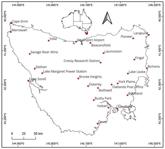
Figure 1. Locations of the selected stations used to estimate the GEV distribution shape parameter.

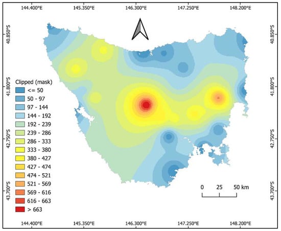
Figure 2. Topography of Tasmania based on the elevations of the selected stations.

The topographic map (Figure 2) of the state suggests that the topography of the state is mostly rugged. The central plateau of the state is at a high altitude, and mountains cover most of the central-west. The coastal regions are at a low altitude, except for some regions in the north-west and eastern parts of Tasmania. The north-west side of the state is confined by extensive flood plains.

3. Methods

The study was conducted by applying the traditional GEV distribution function of the EVT [27]. Although there exists much research investigating numerous candidate distributions for modelling and analysing extreme values, this study emphasises the GEV distribution due to its theoretical foundation in EVT and its extensive adoption in hydrological practices. The GEV distribution offers flexibility in modelling tail behaviour through the shape parameter, making it appropriate for analysing extreme rainfall events [27,28,29].

The EVT technique implements an integrated methodology for analysing both seasonal and spatial alterations in the shape parameters of the widely used GEV distribution across Tasmania. While previous research has predominantly been dedicated to either seasonal or spatial variability, thorough evaluations integrating these dimensions remain inadequate. The overall method specifies a more comprehensive representation of extreme rainfall behaviour and improves the applicability of the outcomes for regional flood risk assessment. Additionally, the literature focusing on the behaviour of the shape parameter, which is essential for distinguishing the tail behaviours of the probabilities of extreme events, is limited. By investigating its variability across seasons and localities, this research provides new insights into the dynamics of hydrological extremes and contributes to advancing regional flood risk investigations.

The three main steps involved in fitting the EVT were as follows: (i) the selection of extreme data series satisfying certain statistical criteria (large sample sizes, i.e., more than 30 years, independent data sets), (ii) the use of the selected data to fit the best probability distribution model, and (iii) the application of the fitted model to generate statistical interpretation maps regarding the underlying population. This study extended the study conducted by Hossain et al. [13]. For a more comprehensive perspective, the length of the data series and the number of meteorological stations were increased. The study conducted by Hossain et al. [13] was based on a data series from 1965 to 2018 at 12 meteorological stations. The analysis in this study was performed on a data series from 1941 to 2019 at 26 meteorological stations.

The extreme data sets for each of the stations were chosen using the block maxima approach. Since the focus was on seasonal variation in the GEV distribution shape parameter, each of the seasons was considered to be the length of the corresponding block. As a result, the maximum precipitation for each season was chosen as the extreme for that season. It is worth noting that the annual maximum series of the seasonal rainfall were assumed to be stationary, since no substantial trends were projected within the study period. As the objective of the study was the investigation of seasonal and spatial differences in the GEV distribution shape parameter, the adoption of stationary assumptions in extreme data sets ensured that the estimation of the shape parameter was comparable among seasons and locations. However, the probable impacts of climate-related non-stationarity are acknowledged as a constraint of the current research. No outliers have been removed from the data sets, as all extreme values represent actual flood events rather than errors in the measurements. The independence of the seasonal maximum data sets was maintained using non-overlapping windows so that individual observations influenced at most one seasonal maximum.

The GEV distribution was fitted for each of the seasons to determine the parameters of the distribution, as shown in Equation (1), as follows:

$$G\left(Y,\theta \right)=exp\left\{-{\left[1+\xi \left({\displaystyle \frac{Y-\mu }{\sigma }}\right)\right]}^{-1/\xi }\right\}$$

(1)

where $Y$ is extreme precipitation, $\theta$ is the parameters of the GEV distribution, which are demonstrated as $\theta \left(\mu ,\sigma ,\xi \right)$, where $\mu$ is the location parameter, $\sigma$ is the scale parameter, and $\xi$ is the shape parameter. The location and scale parameters vary according to the geographical location of the stations, depending on the dryness or wetness of the area, and the variability of the extreme rainfall [23]. According to the study by Koutsoyiannis [21], the shape parameters should be the same for all stations. Therefore, the study investigated the magnitude of the shape parameters for different stations and their variations between seasons.

To investigate the appropriateness of the parameters, four GEV distribution parameter estimation techniques were used in this research: MLE, GMLE, Bayesian, and L-moments. A description of the methods can be revisited in [27].

The shape parameter of the GEV distribution has the potential to be significantly altered by asymmetry in the data, specifically L-skewness, when adopting the L-moments method. The mathematics for calculating the parameters of the GEV distribution using MLE, GMLE, Bayesian estimation, and L-moments are well acknowledged in the literature. For comprehensive derivations and equations, readers are referred to [15,27,30,31,32,33]. These sources specify detailed descriptions of the approximation process and the link between the shape parameter and data asymmetry.

Finally, the spatial analysis of the magnitude of the shape parameter was performed to show the probable GEV type throughout Tasmania. Spatial mapping of the shape parameter was performed by implementing the Inverse Distance Weighting (IDW) method, which approximates the magnitudes of the GEV distribution shape parameters at unsampled sites, considering the spatial correlation of estimated data points. The method is frequently adopted in hydrological research for capturing the spatial variability of modelling parameters. The analysis was performed separately for different seasons using the geographical locations (latitude, longitude, elevation) of the meteorological stations.

4. Results and Discussion

Understanding the climatology of a region is beneficial for understanding the nature of climatic extreme events. Table 2 shows the descriptive statistics (average, maximum, and coefficient of variation) of Tasmanian daily rainfall for the designated duration. According to Table 2, among all the stations analysed, the maximum average rainfall was observed for station #9720 (Lake Margaret Power Station), and the absolute maximum rainfall was observed for station #91109 (Yolla (Sea View) station). With regard to the lowest value, the minimum mean was observed for station #95001 (Bothwell (Franklin Street) station), and the lowest maximum was observed for station #95003 (Bushy Park (Bushy Park Estates) station). In general, the maximum rainfall for the study period did not depend on the maximum average daily rainfall. For example, station 91109 had the highest absolute maximum rainfall (248.00 mm), whereas its average daily rainfall was lower (i.e., 3.91 mm). As extreme rainfall events are rare (e.g., 1 in 100-year events), they have less influence on impacting the average.

Table 2. Statistics on daily rainfall (1941 to 2019) used in this study.

Station Number	Mean Daily Rain	Maximum Daily Rain	Coefficient of Variation
91001	2.59	143.50	2.53
91011	2.58	110.70	2.05
91022	1.71	106.40	2.72
91072	1.87	86.20	2.68
91109	3.91	248.00	2.16
91126	2.12	135.10	2.59
91223	3.03	100.60	1.79
92003	1.91	175.70	3.51
92006	1.72	143.20	3.42
92012	1.65	121.60	3.33
92019	2.26	193.00	2.90
92030	2.65	142.40	2.59
92045	2.04	210.60	2.87
93007	1.48	82.00	2.88
93014	1.44	104.90	2.89
94020	2.39	121.40	2.24
94031	2.26	223.30	2.82
94061	1.51	127.00	3.01
95001	1.43	86.90	2.75
95003	1.55	66.00	2.40
95016	1.90	111.00	2.51
96002	2.48	104.10	2.04
97000	3.66	78.00	1.59
97020	8.25	119.40	1.44
97047	5.38	96.80	1.47
97054	6.65	125.20	1.49

In addition, the coefficient of variation in the daily rainfall data is relatively small across the data series compared with the mean values. Therefore, the data can be used confidently to determine the probability of the occurrence of extreme rainfall.

While Table 2 outlines key statistical summaries (e.g., mean daily rainfall, maximum daily rainfall, and coefficient of variation) that are applicable to the scope of this paper, higher-order indicators, such as skewness, L-skewness, kurtosis, and L-kurtosis, play a significant role in the choice of distribution when using L-moments for parameter estimation. These were not incorporated in this study to uphold an emphasis on parameter estimation methods for the GEV distribution. Nevertheless, future research should combine these statistics for a more thorough evaluation of GEV distribution parameters [32,34,35].

The main objective of this paper was the investigation of the variation in the GEV distribution shape parameter and the selection of an appropriate GEV type in extreme event modelling. The outcomes of the research reveal that a constant shape parameter should not be adopted for Tasmania, and oppose the findings of the investigation by Koutsoyiannis [21]. Like the location and scale parameters, the shape parameter of the GEV distribution varies from one location to another, and hence, so does the type of GEV distribution. As regional variations in the GEV distribution shape parameter exist [23], the type of GEV to be adopted in extreme event modelling must be different from one location to another.

Figure 3 shows the plot of seasonal variations in the magnitude of the shape parameter for the selected meteorological stations. The variations are shown separately for the four different seasons and for parameters estimated using the four different methods. Figure 3 clearly demonstrates that the shape parameter is more than zero for most of the stations in Tasmania for all four seasons. This establishes that the Fréchet (type II) distribution is appropriate in most of the regions of Tasmania. However, there are a few areas where the magnitude of the shape parameter was found to be less than zero, indicating the appropriateness of the Weibull (type III) distribution. For example, a negative shape parameter was observed in summer for station #93007 and station #94061; in autumn for station #91072 and station #97000; in winter for station #91011, station #95003, station #95016, and station #96002; and in spring for station #91011, station #950003, and station #97047. Furthermore, variations in the shape parameter were observed with the parameter estimation techniques. As such, for station #93007, a positive shape parameter was observed with the MLE and Bayesian parameter estimation methods, whereas a negative shape parameter was observed with the GMLE and L-moments methods. This implies that the type of GEV distribution depends on location, season, and even the GEV distribution parameter estimation technique. Therefore, the selection of an appropriate GEV distribution parameter estimation technique is essential in hydrologic applications. Fundamentally, as opposed to Ragulina and Reitan [23], the common regional GEV type is not suitable for extreme rainfall modelling. The unevenness of the area may have a significant influence on the magnitude of the shape parameter rather than its height above the mean sea level. Inherently, the regional smoothing applied by Australian Rainfall and Runoff (ARR) is the appropriate option when estimating design rainfall using the GEV distribution.

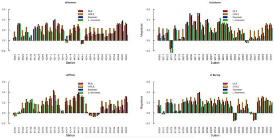
Figure 3. Magnitude of the shape parameters for all four seasons in Tasmania.

Furthermore, Papalexiou and Koutsoyiannis [22] recommended that the value of the shape parameter be from 0 to 0.23. Due to the spatial variation in climatic parameters, it is potentially possible to have different shape parameters in the southern hemisphere. This study demonstrated that the largest value of the shape parameters varies by season. The maximum value of the shape parameter was observed to be 0.406, 0.521, 0.437, and 0.404 in summer, autumn, winter, and spring, respectively. In summer and spring, the largest shape parameter was observed using the Bayesian method, whereas in autumn and winter, the maximum value was observed using the MLE method. This may be due to the length of the data series used to estimate the shape parameter. Papalexiou and Koutsoyiannis [22] analysed a data series ranging from 40 to 63 years. This study concentrated on an extreme data series spanning 79 years (1941 to 2019). Another reason for the dissimilar shape parameters may be due to the different geographical regions.

As there is strong evidence of the regional differences in the shape parameters of the GEV distribution, further investigation of the magnitude of the shape parameter was performed by applying spatial analysis. As the meteorological stations are distributed all over Tasmania, the analysis was able to extract the spatial patterns and characteristics of the shape parameters across the state. Spatial variations in the shape parameters with the seasons are shown in Figure 4, Figure 5, Figure 6 and Figure 7 for the MLE, GMLE, Bayesian, and L-moments methods, respectively.

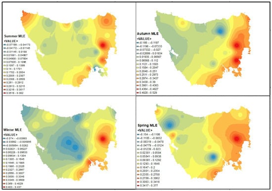
Figure 4. Spatial variation in GEV Distribution shape parameter using MLE method.

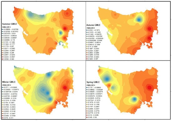
Figure 5. Spatial variation in GEV distribution shape parameter using GMLE method.

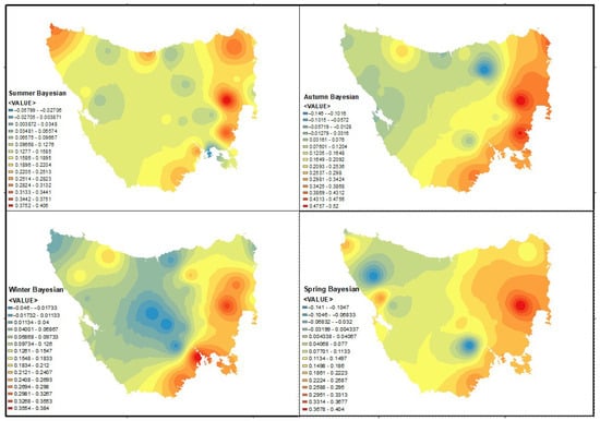
Figure 6. Spatial variation in GEV distribution shape parameter using Bayesian method.

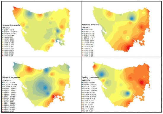
Figure 7. Spatial variation in GEV distribution shape parameter using L-moments method.

From Figure 4, Figure 5, Figure 6 and Figure 7, it is demonstrated that the eastern part of Tasmania has a higher value in its shape parameter when compared with the other parts. Nevertheless, the variation changes with the seasons, as evidenced by the spatial maps. The central part shows significantly lower (negative) shape parameter values when compared with the eastern part. This argument is especially true for winter, implying that the decay of the upper tail of the distribution has an upper bound. Therefore, in the central region, the Weibull-type GEV distribution is appropriate during winter. This observation is valid for the northern region as well. The assertion holds true for all of the GEV distribution parameter estimation techniques. The large number of lakes and mountains in the central parts of Tasmania may have contributed to its negative shape parameter.

It is evident from the spatial analysis that the shape parameters are different from one station to another. For example, the shape parameter tends to be negative in winter and positive in other seasons (summer, autumn, spring) in the central region of Tasmania, as shown in Figure 4, Figure 5, Figure 6 and Figure 7. A similar observation could be made for the north-western region of Tasmania. It is also evident that neither the location nor the proximity to the ocean has a significant influence on the magnitude of the shape parameter. As such, positive shape parameters were observed in the eastern region across all seasons. Therefore, the eastern region of the state has the potential to face more extreme rainfall, leading to hazards. However, a negative shape parameter was observed in the central-western region during winter, leading to fewer hazards compared to the eastern region.

The spatial irregularity of the shape parameters reflected in this study potentially represents the influences of inherent physical and climatic conditions. Areas with higher altitudes and complex landscapes have the potential to demonstrate heavy tails, which can be ascribed to orographic lifting, which induces increased precipitation intensity during frontal systems [36,37]. Likewise, large-scale atmospheric flow patterns and moisture carriage paths play an important role in seasonal rainfall extremes. Furthermore, westerly flows and moisture-laden air masses have a significant influence on the increased extremes in the climate of the western region of Tasmania [38]. The dominant storm types also have an influence; areas regularly impacted by convective storms may possess larger irregularities in their shape parameters compared to areas governed by stratiform precipitation [39]. While a comprehensive attribution analysis was outside the scope of this paper, these physical features offer reasonable explanations for the geographic distribution of the shape parameters, which highlights the necessity of combined hydro-climatological evaluations in future research.

Furthermore, the elevation does not have a profound impact on the shape parameter across all seasons. In the central region at high altitudes, the shape parameter decreased in winter, and the magnitude became negative. The probable effects of cool and gusty weather in winter led to the upper-bound GEV distribution in the central mountainous range. However, this statement is not valid for the other three seasons. Although the central-east has mountainous regions, a positive shape parameter was observed across all seasons. The magnitude changed with the seasons, supporting the hypothesis of seasonal variation in the shape parameter. However, there was an insignificant impact of the latitude on the shape parameter, as suggested by Ragulina and Reitan [23]. Consequently, a common shape parameter is not appropriate for all stations. There may be non-linear relationships between the magnitude of the shape parameter and elevation, as demonstrated by the higher shape parameter in the northern region with a lower elevation (8.0 m at Devonport Airport), and the lower shape parameter in the central region with a higher elevation (710.0 m at Bronte Heights).

The ruggedness of the area may have an impact on the magnitude of the shape parameter and, hence, the selection of an appropriate GEV type. However, it is very difficult to control the roughness of an area and its controlling factors. Furthermore, the characteristics of an area may change over time, which has the potential to change the extreme climatic events of the area. Therefore, regional analysis is the priority in the hydrology of extreme events, as evidenced by the changes in the shape parameter and GEV type in this study.

The accuracy of the assumed distribution was assessed by the commonly used quantile–quantile (QQ) plot. Seasonal variations in the quantile plot are shown in Figure 8 for station #91011 for all parameter estimation techniques. According to Figure 8, the empirical quantiles and model quantiles are within the 45° line, indicating that the GEV distribution characterises the seasonal extreme rainfall accurately.

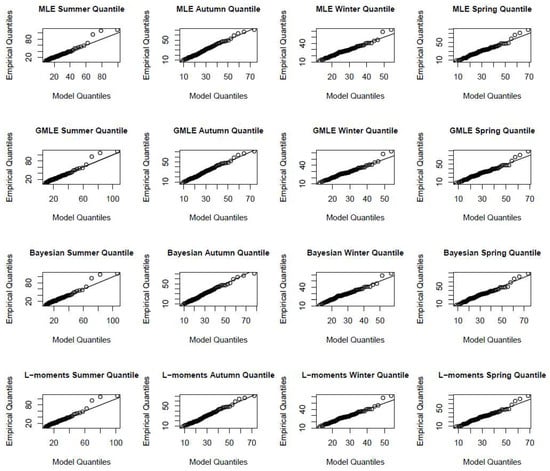
Figure 8. Seasonal variation in goodness-of-fit test for meteorological station #91011.

The determination of climatic risk was performed by estimating the return levels for different recurrence intervals. Return levels of extreme rainfall for the current study are shown in Table 3. As Hossain et al. [13] noted that the L-moments method is best for hydrologic calculation, the return levels are shown using the L-moments method. Khastagir et al. [40] also recommended using the L-moments method in extreme bushfire modelling. It is evident from the table that the return level of extreme rainfall varies with seasons. Like the actual rainfall, there are spatial and temporal variations in the future rainfall. For a 100-year return period, the maximum return level would be observed at station #94031 in summer; whereas in autumn and winter, the 100-year maximum return would be at station #92019; and in spring, the maximum return level would be at station #92033.

Table 3. Seasonal variation in return level estimation using L-moments method.

Station Number	Summer						Autumn						Winter						Spring
	T = 2	T = 5	T = 10	T = 20	T = 50	T = 100	T = 2	T = 5	T = 10	T = 20	T = 50	T = 100	T = 2	T = 5	T = 10	T = 20	T = 50	T = 100	T = 2	T = 5	T = 10	T = 20	T = 50	T = 100
91001	32.9	47.5	57.5	67.6	81.1	91.7	34.0	48.4	58.3	68.1	81.2	91.4	36.6	48.8	56.5	63.6	72.3	78.5	30.3	44.7	55.6	67.2	84.1	98.4
91011	22.8	36.0	47.8	62.1	86.4	110.1	26.4	38.5	46.9	55.2	66.4	75.1	26.0	34.0	39.3	44.3	50.6	55.3	28.1	39.9	47.6	54.8	64.0	70.7
91022	25.7	37.0	45.1	53.4	65.0	74.3	24.3	35.8	45.0	55.3	71.0	84.9	22.2	31.4	38.1	44.9	54.3	61.9	22.4	32.2	40.0	48.7	61.9	73.5
91072	25.8	38.1	47.6	57.8	72.7	85.4	28.0	36.9	41.6	45.4	49.5	52.0	25.0	35.4	43.7	53.0	67.3	80.0	23.0	31.4	37.9	45.0	55.4	64.2
91109	37.4	54.2	65.3	76.0	89.8	100.2	41.0	60.4	75.8	92.8	118.7	141.4	45.7	63.5	78.6	96.2	124.6	151.0	38.9	52.9	62.5	72.0	84.6	94.4
91126	27.2	41.7	53.5	66.9	87.9	106.7	29.1	41.1	49.3	57.2	67.7	75.7	27.9	38.5	46.8	55.7	69.1	80.6	26.4	37.4	44.9	52.4	62.5	70.4
91223	23.9	36.8	47.4	59.2	77.5	93.9	27.9	39.1	46.9	54.7	65.1	73.3	27.6	36.3	42.1	47.7	55.0	60.5	25.7	36.2	44.8	54.4	69.2	82.5
92003	38.1	63.7	82.2	101.1	127.6	149.1	33.9	55.8	74.7	97.0	133.5	167.8	31.6	49.9	63.9	79.0	101.3	120.3	32.6	52.8	68.6	85.9	111.8	134.3
92006	33.4	56.0	73.8	93.3	122.7	148.4	27.0	49.2	68.6	91.6	129.5	165.6	30.6	50.5	65.7	82.0	106.0	126.3	26.9	42.8	55.1	68.4	87.9	104.7
92012	31.2	51.0	66.2	82.6	106.8	127.4	28.5	48.8	65.1	83.1	110.8	135.3	27.6	45.2	58.5	72.5	92.8	109.7	23.6	36.8	46.9	57.8	73.9	87.5
92019	28.1	44.9	58.5	73.9	97.8	119.2	31.3	56.8	80.0	108.6	158.0	206.9	32.8	56.6	76.1	98.2	132.7	163.8	27.1	42.2	55.1	70.1	94.4	117.0
92030	35.0	55.5	70.9	87.2	110.8	130.5	38.2	58.7	73.7	89.2	111.2	129.1	35.9	50.1	60.2	70.5	84.7	96.0	32.0	45.7	56.2	67.6	84.4	98.8
92045	31.3	49.9	64.4	80.4	104.4	125.3	30.1	51.5	71.0	94.9	136.0	176.6	27.3	40.2	48.7	56.8	67.3	75.1	28.8	44.4	57.2	71.6	93.9	113.9
93007	27.4	40.5	48.9	56.8	66.6	73.7	22.1	34.1	43.3	53.2	67.8	80.3	19.8	31.2	39.8	49.0	62.5	73.7	21.4	31.7	39.5	47.6	59.4	69.1
93014	25.2	38.5	48.4	58.9	74.1	86.8	21.9	34.1	43.6	53.8	69.0	82.0	19.5	30.0	37.7	45.8	57.2	66.5	20.4	31.0	39.2	47.9	60.8	71.7
94020	27.9	43.3	55.4	68.7	88.5	105.8	21.3	33.0	44.6	59.8	87.7	117.3	26.9	40.0	50.6	62.6	81.2	97.9	25.7	37.9	47.5	58.3	74.8	89.3
94031	31.6	53.3	71.0	90.9	122.0	149.9	28.1	48.0	66.2	88.6	127.2	165.4	29.4	46.6	62.2	81.3	114.1	146.4	29.3	44.1	55.4	67.5	85.0	99.8
94061	29.5	43.7	52.6	60.7	70.8	78.0	22.8	37.8	50.5	65.1	88.5	109.9	20.0	31.9	42.5	55.2	76.3	96.6	22.1	34.6	44.3	55.0	71.0	84.9
95001	23.6	36.9	46.3	55.8	68.8	79.1	21.0	32.5	41.0	50.1	63.0	73.7	19.8	28.7	34.7	40.5	48.1	53.8	19.7	28.2	34.5	41.1	50.4	58.1
95003	21.1	31.6	39.1	46.8	57.4	65.9	19.4	28.4	34.6	40.9	49.4	56.1	18.9	26.0	30.5	34.7	39.9	43.7	19.3	24.6	27.8	30.5	33.7	35.9
95016	23.0	34.8	43.3	52.1	64.5	74.5	23.6	35.5	44.8	55.0	70.4	83.7	24.5	33.7	39.5	44.7	51.1	55.6	24.8	34.3	41.0	47.7	56.8	63.9
96002	24.0	35.8	44.6	53.7	66.7	77.5	24.5	33.8	40.8	48.2	58.9	67.8	25.8	34.5	40.2	45.6	52.4	57.5	24.4	32.0	37.3	42.6	49.7	55.2
97000	25.2	34.7	41.8	49.1	59.7	68.5	29.9	38.2	43.4	48.3	54.4	58.8	31.6	41.9	49.4	57.3	68.4	77.5	26.2	34.6	40.6	46.8	55.4	62.3
97020	48.2	62.5	72.8	83.2	97.7	109.2	56.4	71.9	82.7	93.5	107.9	119.2	52.7	66.1	75.6	85.3	98.6	109.3	50.6	62.0	69.3	76.3	85.2	91.8
97047	32.3	44.9	54.4	64.3	78.5	90.4	37.2	48.2	55.7	63.0	72.7	80.2	36.9	46.4	53.8	61.9	73.9	84.2	35.0	42.3	46.6	50.4	54.7	57.7
97054	38.4	52.5	63.5	75.6	93.8	109.5	47.3	60.3	69.2	78.0	89.6	98.5	46.7	57.6	65.8	74.5	87.1	97.5	41.8	52.8	61.1	69.7	82.2	92.5

5. Conclusions and Recommendations

This study evaluates the seasonal variability of the GEV distribution shape parameter and its influence on extreme precipitation modelling. To fulfil the objectives of the research, daily precipitation data from 26 meteorological stations in Tasmania were used. Seasonal extreme data sets were obtained using the block maxima approach and fitted to the GEV distribution. The parameters of the distribution were obtained using the MLE, GMLE, Bayesian, and L-moments methods. A spatial analysis of the parameters was performed and was provided using GIS interpolation maps. Subsequently, as the selected stations were distributed across the state, a spatial model was considered in the analysis. The conclusion of the study can be summarised as follows:

• There exist significant variations in the shape parameters among the 26 rain gauge stations across Tasmania. The maximum and minimum values of the shape parameter throughout Tasmania were obtained—0.234 and 0.529. Hence, the adoption of the GEV type varies among seasons for extreme rainfall modelling. As such, a regionally common value of the shape parameter should not be considered when determining design rainfall. The shape parameter has the potential to decrease with elevation. A similar outcome was obtained by Ragulina and Reitan [23] for the shape parameter.
• The magnitude of the parameter is significantly different from one season to another. The governing precipitation system of a region may have the potential to create seasonal variation in the shape parameter. Nevertheless, more research is required to identify the seasonal trends in shape parameters.
• Spatial analysis of the shape parameter suggests that using Weibull-type GEV distribution is appropriate in the central and northern regions of Tasmania during the winter. However, the type of GEV distribution varies with the season.
• Finally, the most dominant factor influencing the shape parameter has yet to be identified. Climate change may have a significant influence on the magnitude of the shape parameter. Therefore, further investigation is essential to establish the dependency of the shape parameter on this variable.

Future research has the potential to combine the K-moment method [41,42] together with L-moments and other estimation techniques to deliver a more comprehensive evaluation of parameter estimation techniques for the GEV distribution. This has the potential to assess the comparative strength and efficacy of K-moments under variable sample sizes and hydrological conditions.

References

- IPCC. Climate Change 2014: Synthesis Report. Contribution of Working Groups I, II and III to the Fifth Assessment Report of the Intergovernmental Panel on Climate Change; IPCC: Geneva, Switzerland, 2014. [Google Scholar]
- Fish, E. The Forgotten Legacy of the Banqiao Dam Collapse. The Economic Observer, 8 February 2013. [Google Scholar]
- Blanchet, J.; Marty, C.; Lehning, M. Extreme value statistics of snowfall in the Swiss Alpine region. Water Resour. Res. 2009, 45, W05424. [Google Scholar] [CrossRef]
- Coles, S.G.; Tawn, J.A. A Bayesian analysis of extreme rainfall data. J. R. Stat. Soc. 1996, 45, 463–478. [Google Scholar] [CrossRef]
- Dyrrdal, A.V.; Skaugen, T.; Stordal, F.; Førland, E.J. Estimating extreme areal precipitation in Norway from a gridded dataset. Hydrol. Sci. J. 2016, 61, 483–494. [Google Scholar] [CrossRef]
- Hossain, I.; Esha, R.; Alam Imteaz, M. An Attempt to Use Non-Linear Regression Modelling Technique in Long-Term Seasonal Rainfall Forecasting for Australian Capital Territory. Geosciences 2018, 8, 282. [Google Scholar] [CrossRef]
- Hossain, I.; Rasel, H.M.; Imteaz, M.A.; Mekanik, F. Long-term seasonal rainfall forecasting using linear and non-linear modelling approaches: A case study for Western Australia. Meteorol. Atmos. Phys. 2020, 132, 331–341. [Google Scholar] [CrossRef]
- Hossain, I.; Rasel, H.M.; Mekanik, F.; Imteaz, M.A. Artificial neural network modelling technique in predicting Western Australian seasonal rainfall. Int. J. Water 2020, 14, 14–28. [Google Scholar] [CrossRef]
- El Adlouni, S.; Ouarda, T.B.M.J. Frequency analysis of extreme rainfall events. Rainfall State Sci. 2010, 191, 171–188. [Google Scholar]
- Katz, R.W.; Parlange, M.B.; Naveau, P. Statistics of extremes in hydrology. Adv. Water Resour. 2002, 25, 1287–1304. [Google Scholar] [CrossRef]
- Yilmaz, A.G.; Hossain, I.; Perera, B.J.C. Effect of climate change and variability on extreme rainfall intensity–frequency–duration relationships: A case study of Melbourne. Hydrol. Earth Syst. Sci. 2014, 18, 4065–4076. [Google Scholar] [CrossRef]
- Cannon, A.J.; Innocenti, S. Projected intensification of sub-daily and daily rainfall extremes in convection-permitting climate model simulations over North America: Implications for future intensity–duration–frequency curves. Nat. Hazards Earth Syst. Sci. 2019, 19, 421–440. [Google Scholar] [CrossRef]
- Hossain, I.; Imteaz, M.A.; Khastagir, A. Effects of estimation techniques on generalised extreme value distribution (GEVD) parameters and their spatio-temporal variations. Stoch. Environ. Res. Risk Assess. 2021, 35, 2303–2312. [Google Scholar] [CrossRef]
- Bhunya, P.K.; Jain, S.K.; Ojha, C.S.; Agarwal, A. Simple parameter estimation technique for three-parameter generalized extreme value distribution. J. Hydrol. Eng. 2007, 12, 682–689. [Google Scholar] [CrossRef]
- Coles, S.G.; Dixon, M.J. Likelihood-Based Inference for Extreme Value Models. Extremes 1999, 2, 5–23. [Google Scholar] [CrossRef]
- Park, J.-S. A simulation-based hyperparameter selection for quantile estimation of the generalized extreme value distribution. Math. Comput. Simul. 2005, 70, 227–234. [Google Scholar] [CrossRef]
- Lazoglou, G.; Anagnostopoulou, C. An overview of statistical methods for studying the extreme rainfalls in Mediterranean. Proceedings 2017, 1, 681. [Google Scholar] [CrossRef]
- Anghel, C.G.; Ianculescu, D. Probabilistic Forecasting of Peak Discharges Using L-Moments and Multi-Parameter Statistical Models. Water 2025, 17, 1908. [Google Scholar] [CrossRef]
- Bora, D.J.; Borah, M.; Bhuyan, A. Regional analysis of maximum rainfall using L-moment and LH-moment: A comparative case study for the northeast India. Mausam 2017, 68, 451–462. [Google Scholar] [CrossRef]
- Guttman, N.B. The use of L-moments in the determination of regional precipitation climates. J. Clim. 1993, 6, 2309–2325. [Google Scholar] [CrossRef]
- Koutsoyiannis, D. Statistics of extremes and estimation of extreme rainfall: I. Theoretical investigation/Statistiques de valeurs extrêmes et estimation de précipitations extrêmes: I. Recherche théorique. Hydrol. Sci. J. 2004, 49, 575–590. [Google Scholar] [CrossRef]
- Papalexiou, S.M.; Koutsoyiannis, D. Battle of extreme value distributions: A global survey on extreme daily rainfall. Water Resour. Res. 2013, 49, 187–201. [Google Scholar] [CrossRef]
- Ragulina, G.; Reitan, T. Generalized extreme value shape parameter and its nature for extreme precipitation using long time series and the Bayesian approach. Hydrol. Sci. J. 2017, 62, 863–879. [Google Scholar] [CrossRef]
- Villarini, G.; Smith, J.A. Flood peak distributions for the eastern United States. Water Resour. Res. 2010, 46, 863–879. [Google Scholar] [CrossRef]
- Tyralis, H.; Papacharalampous, G.; Tantanee, S. How to explain and predict the shape parameter of the generalized extreme value distribution of streamflow extremes using a big dataset. J. Hydrol. 2019, 574, 628–645. [Google Scholar] [CrossRef]
- El Adlouni, S.; Ouarda, T.B.M.J.; Zhang, X.; Roy, R.; Bobée, B. Generalized maximum likelihood estimators for the nonstationary generalized extreme value model. Water Resour. Res. 2007, 43, W03410. [Google Scholar] [CrossRef]
- Coles, S. An Introduction to Statistical Modeling of Extreme Values; Springer: New York, NY, USA, 2001. [Google Scholar]
- Chen, J.; Sayama, T.; Yamada, M.; Sugawara, Y. Regional event-based flood quantile estimation method for large climate projection ensembles. Prog. Earth Planet. Sci. 2024, 11, 16. [Google Scholar] [CrossRef]
- Hiraga, Y.; Iseri, Y.; Warner, M.D.; Duren, A.M.; England, J.F.; Frans, C.D.; Kavvas, M.L. Model-based estimation of long-duration design precipitation for basins with large storage volumes of reservoirs and snowpacks. J. Flood Risk Manag. 2024, 17, e12992. [Google Scholar] [CrossRef]
- Coles, S.; Tawn, J. Bayesian modelling of extreme surges on the UK east coast. Philos. Trans. R. Soc. A Math. Phys. Eng. Sci. 2005, 363, 1387–1406. [Google Scholar] [CrossRef]
- Hosking, J.R.M. L-Moments: Analysis and Estimation of Distributions Using Linear Combinations of Order Statistics. J. R. Stat. Soc. Ser. B Methodol. 1990, 52, 105–124. [Google Scholar] [CrossRef]
- Hosking, J.R.M.; Wallis, J.R. Regional Frequency Analysis: An Approach Based on L-Moments; Cambridge University Press: Cambridge, UK, 1997. [Google Scholar]
- Hossain, I.; Khastagir, A.; Aktar, M.N.; Imteaz, M.A.; Huda, D.; Rasel, H.M. Comparison of estimation techniques for generalised extreme value (GEV) distribution parameters: A case study with Tasmanian rainfall. Int. J. Environ. Sci. Technol. 2022, 19, 7737–7750. [Google Scholar] [CrossRef]
- Ilinca, C.; Stanca, S.C.; Anghel, C.G. Assessing Flood Risk: LH-Moments Method and Univariate Probability Distributions in Flood Frequency Analysis. Water 2023, 15, 3510. [Google Scholar] [CrossRef]
- Anghel, C.G.; Stanca, S.C.; Ilinca, C. Extreme Events Analysis Using LH-Moments Method and Quantile Function Family. Hydrology 2023, 10, 159. [Google Scholar] [CrossRef]
- Smith, R.B.; Jiang, Q.; Fearon, M.G.; Tabary, P.; Dorninger, M.; Doyle, J.D.; Benoit, R. Orographic precipitation and air mass transformation: An Alpine example. Q. J. R. Meteorol. Soc. 2003, 129, 433–454. [Google Scholar] [CrossRef]
- Roe, G.H. Orographic precipitation. Annu. Rev. Earth Planet. Sci. 2005, 33, 645–671. [Google Scholar] [CrossRef]
- Department of Primar y Industries, Parks, Water and Environment (DPIPWE). Vulnerability of Tasmania’s Natural Environment to Climate Change: An Overview; Department of Primar y Industries, Parks, Water and Environment: Hobart, Australia, 2010. [Google Scholar]
- Trenberth, K.E.; Dai, A.; Rasmussen, R.M.; Parsons, D.B. The changing character of precipitation. Bull. Am. Meteorol. Soc. 2003, 84, 1205–1218. [Google Scholar] [CrossRef]
- Khastagir, A.; Hossain, I.; Aktar, N. Evaluation of different parameter estimation techniques in extreme bushfire modelling for Victoria, Australia. Urban Clim. 2021, 37, 100862. [Google Scholar] [CrossRef]
- Koutsoyiannis, D. Knowable moments for high-order stochastic characterization and modelling of hydrological processes. Hydrol. Sci. J. 2019, 64, 19–33. [Google Scholar] [CrossRef]
- Ianculescu, D.; Anghel, C.G. Innovative Explicit Relations for Weibull Distribution Parameters Based on K-Moments. Mathematics 2025, 13, 3473. [Google Scholar] [CrossRef]
Disclaimer/Publisher’s Note: The statements, opinions and data contained in all publications are solely those of the individual author(s) and contributor(s) and not of MDPI and/or the editor(s). MDPI and/or the editor(s) disclaim responsibility for any injury to people or property resulting from any ideas, methods, instructions or products referred to in the content. |
© 2026 by the authors. Licensee MDPI, Basel, Switzerland. This article is an open access article distributed under the terms and conditions of the Creative Commons Attribution (CC BY) license.