Determination of the Surface Watercourse Velocities by Using the Propeller Current Meter, Unmanned Aerial Vehicle, and Mobile Phone

Abstract

According to existing procedures for defining the velocity distribution across cross profile sections of watercourses (e.g., Entropy theory and Power Law theory), surface velocity is a key input parameter, together with cross-sectional bathymetry. Field measurements to obtain velocity values and their distributions are often difficult due to limited equipment, unreliable data, missing data, or hazardous conditions such as flooding and inaccessible locations. This creates a strong need for alternative approaches to measuring surface velocities in rivers. The application of unmanned aerial vehicles (UAVs), mobile phones, and traditional field instruments such as the Propeller Current Meter (PCM) can significantly improve measurement efficiency, especially in situations where conventional methods are not feasible. This paper presents an algorithm for comparing these measurement approaches and quantifying their differences. The methodology is demonstrated using a real case study on the Bednja River in Croatia, which flows through alluvial deposits. The results show that video-based surface velocity estimation using UAV and mobile phone imagery is feasible under real river conditions. Still, its accuracy depends strongly on flow conditions and surface characteristics. While UAV recordings provide reliable results in fast and turbulent flows, mobile phone videos yield more stable performance in smoother flow conditions, where additional surface texture is available from natural tracers.

1. Introduction

Determining watercourse velocity and flow is crucial for water management. Predictions of intensity and occurrence periods justify flood protection, drought reduction, sizing of hydrotechnical facilities, irrigation needs, water supply, and many other applications. Climate change and anthropogenic activities pose challenges for such tasks due to disruptions to the hydrological cycle, which, in turn, affect their modeling. The most significant process is water flow in natural and artificial watercourses, due to the stochastic nature of precipitation and other meteorological parameters.

Flow measurement technology and procedures are generally divided into mechanical, electromagnetic, ultrasound, and radar methods. Different techniques are also used to obtain these technologies’ velocity and flow values. The main task is determining the velocity, which can be readily obtained from the cross-sections. For such tasks, the surface velocities are input data, as are the distributions of velocities across the cross profile sections. The velocity distribution, i.e., the measurement of velocity at different depths and distances across the cross profile, is a more complicated task than determining surface velocities, so this will be elaborated on in this paper.

Surface velocities can be determined using simple methods, such as tracking floating objects. The most used applications are radar and electromechanical instruments, mechanical devices such as Propeller Current Meters (PCM), and ultrasound devices. There are many approaches for determining velocity distributions across cross profiles, such as the Entropy theory [1] and the Law theory [2]. It is essential to obtain the cross-sectional profile area at the surface and at the various points along the cross profiles. Such could be received during velocity measurement and/or by applying surveying methods, total station, and GNSS devices (Global Navigation Satellite System).

This research focuses on determining the surface velocities of the measured cross profiles. To this end, effective methods for determining surface velocities are applied at different cross-sections. The Section 3 explains further details. Also, the study will outline the procedures for fieldwork in the event of inability to access the analyzed sites. Such an event is common during extensive flooding, water overflows, and when the water is not entered for velocity measurements. These extreme examples are shown in Figure 1a,b. It is worth noting that the recorded surface velocity will be used as input to the Entropy model to estimate the cross-sectional velocity distribution and flow discharge. This work will be the second part of the current research.

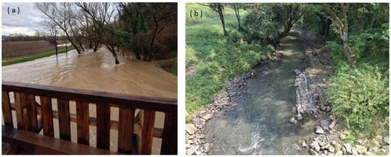
Figure 1. Flow conditions at the analysed site: (a) extreme flow conditions with high water levels; (b) typical flow conditions suitable for conducting measurements.

Figure 1a shows the extreme value of the flow on the analyzed site, while Figure 1b shows a usual (suitable) situation for conducting all measurements. However, modern technologies enable measurement in dangerous situations, such as the one shown in Figure 1a, using measurement devices on a small boat (an Acoustic Doppler Current Profiler—ADCP) or an echosounder. The intention is to provide measurements using equipment suitable for situations like those shown in Figure 1b, as well as to evaluate their performance under different flow conditions. Economic reasons are also taken into account, as are the most important, safety reasons, to avoid any risk of injury or deadly danger to the measurement performers and to the equipment.

These tasks motivate the definition of new procedures for the mentioned problems. In this case, PCM provides reference surface velocities, while UAV and mobile phone recordings are used to derive image-based velocity estimates for comparison. These are much cheaper than ADCPs.

2. Literature Review

The development of UAVs, computer vision, multisensor systems, and radar technologies, as well as non-contact methods for measuring surface velocity and flow, has accelerated significantly over the past decades. Traditional hydrometric instruments—such as ADCPs, electromagnetic current meters, and limnigraphs, although reliable, have limitations due to spatial sampling density, field conditions, inaccessible terrain, or inability to use during floods. Therefore, the application of UAVs is increasingly recognized as a fast, safe, and flexible alternative that can provide hydrometric information in conditions where conventional methods are not able to [3]. Their importance has also increased due to the frequent occurrence of extreme hydrological events, which require rapid and spatially dense monitoring.

As flow estimation is directly related to accurate measurements of watercourse surface velocity, recent research has increasingly focused on UAV methods that provide spatially detailed, operationally feasible velocity measurements.

Optical imaging has become the foundation of UAV hydrometry. Large-Scale Particle Image Velocimetry (LSPIV) allows the detection and tracking of textural features on the water surface. Studies comparing LSPIV measurements with in situ measurements agree within a few centimeters per second [4,5,6]. A significant application of this method is in heterogeneous river systems, where UAV platforms can capture non-contact images of turbulent surface structures, rapids, or flood waves [7]. Research demonstrates that UAV images provide insights into rapid flow variations during flood events [3]. The UAV–LSPIV process includes nadir (90°) or slightly oblique images with dense temporal overlap, geometric correction (orthorectification), and texture shift analysis in the Euler frame. Recent field studies of the UAV–LSPIV method have shown that data quality depends on the geometric configuration of the imaging and the selection of processing parameters. Low-altitude UAV platforms provide more accurate results than conventional cameras, with a mean absolute error of 0.07 m/s or less. Research emphasizes the importance of optimizing the survey window (16 × 16 px) and the sampling interval (1/8 s), which aligns with recent recommendations for UAV-based optical velocimetry [8]. Particle Tracking Velocimetry (PTV) is based on individual trackers that are tracked over time. A fully automated PTV procedure was developed that includes camera motion correction, automatic water surface detection, and integration of SfM models for cross-section extraction [9]. PTV is particularly effective in shallow and small streams and in conditions where natural surface trackers are available [7]. LSPIV and PTV represent methodologically related, but operationally different approaches. LSPIV is more effective in deriving spatially continuous velocity fields, and PTV is more effective at lower velocities and allows for detailed reconstruction of local turbulent structures. The Space–Time Image Velocimetry (STIV) method is effective in streams with limited surface texture. STIV estimates velocity by analyzing the slope of tracks in space–time images [10]. Adaptations of UAV imaging (enhanced LSPIV and STIV), including platform motion corrections based on GNSS position and orientation data, have been developed [11], enabling robust STIV analysis under operational flight conditions.

New research uses RAFT and Farnebäck algorithms to compensate for the lack of trackers and poor surface contrast. The results show stable velocity estimation with relatively small errors [12]. Optical flow methods rely on the presence of visible texture and contrast in the image. When the surface is smooth and brightness patterns are nearly uniform, motion estimation becomes unreliable. Classical differential approaches, such as the Lucas–Kanade method, tend to extract motion mainly at edges or along textured boundaries, while large homogeneous areas provide little usable information for tracking [13]. Reviews of optical flow techniques show that, despite major advances in both classical and deep-learning-based approaches, real-world conditions such as changing illumination, reflections, and regions with weak visual structure still pose serious challenges for accurate motion estimation [14]. In particular, calm water surfaces often lack sufficient texture, which leads to ambiguous or noisy flow estimates.

The use of UAV-based optical flow for river surface velocity measurements has been reported in several recent studies. Using high-resolution UAV video and deep-learning-based optical flow models, surface velocities were estimated with deviations of about 13–27% when compared with in situ electromagnetic current meter measurements [15]. These results suggest that optical flow can provide spatially continuous velocity fields when surface texture is sufficient, even in situations where conventional image velocimetry methods would normally require artificial tracers.

The integration of optical flow with advanced segmentation techniques, such as YOLOv8, has further increased robustness and enabled UAV hydrometry in near real time [16]. The integration of UAV optical data with satellite observations (e.g., Sentinel, Landsat) enables multi-channel analyses of river dynamics [17].

A fundamental limitation of optical techniques is their dependence on lighting conditions and the presence of suitable surface tracers. Thermal infrared (TIR) cameras (although typically of lower spatial resolution) partially address this shortcoming by allowing velocity estimates in low-light or night-time conditions, and by capturing thermal patterns associated with surface flow. Research combining RGB and TIR imagery significantly improves the spatial coverage and integrity of velocity vector fields by compensating for low-contrast areas in RGB imagery [18]. Similarly, multispectral and hyperspectral sensors are used to improve flow estimates. They enhance the identification of shallow zones, vegetation influences, and suspended sediment patterns [11,19].

The use of UAV-based image velocimetry in environmentally complex river settings has been tested using IV-UAV methods in intermittent, shallow Mediterranean streams. These studies showed that surface velocities can be estimated even at very low discharges, but they also pointed out important limitations related to vegetation cover, shallow water depths, and reduced surface visibility, which remain key constraints for practical UAV-based hydrometry [20]. Recent research suggests methods that do not rely on ground control points (GCPs) or artificial tracers. Research has been presented that uses triaxial accelerometers, UAV altimeters, and GNSS measurements to reconstruct survey geometry and derive velocity fields from texture displacements [21].

New research agrees that velocities derived from UAV data can significantly improve the calibration of 2D hydrodynamic models by generating spatially representative datasets that overcome the limitations of in situ measurements [22]. However, the conversion of surface to mean depth velocity remains a problem. It has been shown that conversion coefficients around α ≈ 0.8 work well in straight sections and in meandering or morphologically complex areas, but deterioration is observed [23]. An estimate of the conversion coefficient α is provided, emphasizing that the commonly used values of α = 0.8–0.86 are based on ideal velocity profiles [24]. In real rivers, α can vary from 0.7 to more than 1.1, depending on energy gradients, roughness, wind influence, and bed morphology. Their analysis highlights the need for segment-specific α values, particularly during floods and in shallow, hydraulically complex environments. They emphasize the importance of local calibration and the integration of additional hydrological data when available.

Surface velocities obtained from UAV data were successfully used to develop rating curves (stage–discharge relationships) at locations without conventional hydrometric infrastructure. This confirms the need for model calibration and operational hydrological monitoring [25]. Radar UAV sensors (Doppler and FMCW radar) enable operation in cloudy weather, poor visibility, or a lack of trackers. Although radar systems are currently less common due to complexity and cost, recent research identifies them as robust additions to multisensory UAV hydrometry [5].

The literature shows that UAV hydrometry and flow determination are developing in the direction of multisensory integration (optics, TIR, radar), real-time data processing with the support of machine learning and edge computing. Studies show that surface velocity (derived from UAV imagery) is the primary observed quantity. At the same time, other sensors and methods provide additional information for converting velocity into flow and for interpreting spatial flow dynamics.

The growing significance of video and image velocimetry in hydrology is highlighted by recent research, which also confirms that camera-based methods, including smartphones, are being promoted as a methodologically sound and practically beneficial substitute for conventional hydrometric instruments [26]. Smartphones can efficiently use video analysis to collect surface velocity data and provide precise flow measurements by combining integrated sensors with advanced image processing algorithms [27,28]. One application is a real-time surface velocity (SIV) measurement system for an Android smartphone, which determines position and velocity using the smartphone’s GPS and sensors [27].

This approach overcomes the limitations of standard measurement methods, which require expensive, specialized equipment. The research indicates that in some situations, smartphone-based methods can reach measurement accuracy comparable to that of conventional instruments [29]. The successful use of the Large-Scale Particle Image Velocimetry (LLSPIV) technology, which captures video of the water surface to quantify flow velocities in real time, further supports the idea of deploying cellphones [29]. Approaches have achieved successful results even under challenging circumstances, validating the potential of smartphone-based methods for quick, non-invasive data collection. The successful recording and analysis of surface flow velocities by LSPIV have demonstrated its robustness across a variety of hydrological conditions, with good results in both laboratory and field settings [29,30].

Several studies suggest that smartphone-based methods are equally successful as traditional measurement methods. For instance, by decreasing the impact of external variables, the application of image processing techniques to estimate flow velocities has proven promising in calibrating and improving measurement precision [31,32]. This is particularly crucial in natural watercourses, where surface properties can significantly impair measurement accuracy. By combining state-of-the-art image analysis methods, like optical flow approaches, with real-time video processing, smartphones can adapt to the intricacies of aquatic environments [27,28].

Smartphone-based metrics have some disadvantages despite their apparent advantages. The accuracy of the acquired data is strongly influenced by factors such as sufficient lighting, stable imaging settings, and suitable surface texture [33]. Furthermore, a key hurdle to the broader implementation of these methodologies is the parameter uncertainty found in natural flows [34]. Nonetheless, advances in image processing methods and smartphone technology offer significant potential for further research and improvement in this field [29,35]. Further research extends this knowledge by applying several video and image techniques (PTV, PIV, optical flow/SSIV) on smartphones, including orthorectification, displacement-to-velocity conversion, and geometric calibration.

For example, applying the PTV approach using buoys and smartphone photos in laboratory settings yielded an accuracy of less than 3%. In contrast, field deviations from ADCP in some cases reached 15% [36]. Tests of the DischargeApp application in undersized culverts (15–65 L/s) demonstrated a tendency to overestimate discharge, although the inaccuracy was significantly reduced by correcting the surface velocity for flow depth [37]. Similarly, laboratory trials at flow rates of 20–120 L/s indicated that, in 85% of measurements, the relative error was less than about 15%, providing steady recording and the application of GCP calibration marks [38].

The contribution of mobile applications to the development of applications is further highlighted by research, which developed a system for estimating water level, surface velocity, and flow from just a few seconds of video using a modified traceless PIV method [38]. Field results showed that even with a very cheap mobile device, it is possible to achieve a precision of less than 10% in estimating surface velocity and an accuracy of water level better than 1 cm. This line of research continues with the development of a method for estimating surface velocity and flow from smartphone video footage, combined with information on the bed geometry, emphasizing the method’s non-invasiveness as a key advantage in field conditions [39,40].

The SmartPIV system, which tracks surface bubbles on a bridge using optical flow/PIV algorithms with errors of less than 8%, provides further evidence of the reliability of smartphone-based techniques [41]. Within the international database for image velocimetry on the La Vence River (France), images obtained with a Samsung Galaxy S7 device were also successfully processed using standard procedures (orthorectification, grayscale conversion), confirming the compatibility of mobile devices with established image velocimetry protocols [42].

3. Methodology

The current research aims to determine the surface velocities at the analyzed location by measuring them with a hydrological equipment (PCM-FP211, Global Water Instrumentation, Gold River, CA, USA), surveying drone equipment (UAV-Autel EVO II Dual 320, Autel Robotics Co., Ltd., Shenzhen, China), and a mobile phone. Measurements were conducted on three measured cross profile sections of the analyzed Bednja River. Optical flow (Farnebäck method) is used to interpret recorded video files from the UAV and the mobile phone and determine the distribution of surface velocities in Python (version 3.12.5).

3.1. Measurement of the Surface Velocities with the Propeller Current Meter

The PCM is the oldest known hydrological measuring device. The procedure is based on measuring propeller revolutions and determining the speed from the functional dependence between the two [43]. There are separate manual device versions for shallow watercourses and for deep rivers. The measurement technique is based on measuring velocity at particular stations (distances) from the banks of rivers, with respect to the specific depths at those stations, i.e., verticals. Output results could be documented manually or electronically. In this study, PCM measurements are used as reference (ground-truth) surface velocities for validating UAV- and mobile-phone-based estimates. Figure 2 shows a Propeller Current Meter used to measure surface velocities at the analyzed location.

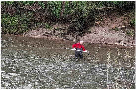
Figure 2. Application of Propeller Current Meter on analyzed location.

The water velocity probe consists of a protected water turbo prop positive displacement sensor, coupled with an expandable probe handle that terminates in a digital readout display. For practical reasons, the Propeller Current Meter is usually used to obtain maximum velocities, which are then presented and analyzed. In this study, the probe was positioned close to the water surface so that the measured maximum near-surface velocity could serve as the reference surface velocity for comparison with the UAV- and mobile-phone-based methods.

3.2. Measurement of the Surface Velocities with a UAV

Unmanned aerial vehicles (UAVs) are used for both civil and scientific purposes, and their ability to operate remotely or autonomously primarily serves as a tool for collecting geospatial data [44,45]. Improvements in materials, battery technology, and computer image processing have driven the development of UAVs, increasing their effectiveness in applications such as photogrammetry, cartography, and water exploration [46,47].

UAV systems are categorized into three groups: multirotor, fixed-wing, and hybrid VTOL designs. In this study, a multirotor UAV was used, as this platform is best suited for hovering and stable video acquisition over a fixed river cross-section. Multirotor UAVs are used for data collection due to their stability, hovering capabilities, and accurate positioning in confined spaces. UAVs can use multiple sensors simultaneously (optical, LiDAR, or IR), enabled by advances in battery technology (lithium-ion systems) that increase energy efficiency and allow the addition of equipment [47,48].

For most surveying tasks, multirotor aircraft typically offer flying durations of 20 to 30 min, which depends on several variables (payload weight, aerodynamic characteristics, and battery capacity). Despite their limitations (flight duration), UAVs remain an accessible source of high-quality data due to their mobility, high spatial resolution, and rapid data-collection capabilities. Because of structural and energy constraints, greater emphasis is being placed on integrating additional navigation systems, such as RTK modules, to enable UAVs to achieve high geolocation accuracy. This also reduces the need to set up numerous ground control points. RTK technology enables the acquisition of precise geographic data, improving the overall accuracy and reliability of the collected information [49].

The UAV recording process begins by connecting the mobile device and the controller using a cable (Figure 3). After inserting the battery into the UAV, we launched the Autel Explorer application on the mobile device, which allowed us to connect to the UAV. The application checks the compass calibration, GPS signal (at least 12 satellites), sensor, and IMU status. Recording parameters were defined within the Camera Settings and Flight Settings menus.

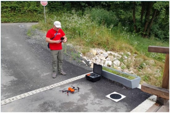
Figure 3. An unmanned aerial vehicle is used to record surface velocity.

The orthophotos were generated from RGB images acquired using the integrated camera of the Autel EVO II Dual platform (camera model reported in the EXIF metadata as XT706). The images were recorded at a resolution of 4000 × 3000 pixels (≈12 MP) with a focal length of f = 5.0 mm and an f/1.8 aperture. The 35 mm equivalent focal length reported in the EXIF data is 26 mm, indicating a wide-angle imaging geometry.

In the nadir case (sensor pointed straight down), the theoretical ground sampling distance (GSD) can be expressed as:

$$GSD={\displaystyle \frac{H\cdot p}{f}}$$

(1)

where H is the flight altitude above ground and p is the physical pixel size on the sensor [50]. Assuming a 1/2″ sensor with a width of W ≈ 6.4 mm and N_x (the horizontal pixel dimension of the digital image), the pixel size is given by:

$$\mathrm{p}={\displaystyle \frac{W}{N_x}}$$

(2)

For H = 60 m, the resulting GSD is 1.92 cm/pixel, which is consistent with the pixel size of the final orthomosaic measured in QGIS (version 3.42.1) (≈1.95 cm/pixel). The deviation of about 1.6% between the theoretically calculated (1.92 cm/pixel) and the obtained spatial resolution (1.95 cm/pixel) can be attributed to variations in actual flight altitude (GNSS/barometric uncertainty and terrain), small differences between nominal and self-calibrated interior orientation parameters (focal length, principal point, distortion) estimated during bundle adjustment, and resampling effects during mosaicking and orthorectification onto the DSM/DTM.

Using the measured orthomosaic resolution GSD ≈ 0.0195 m/pixel, each photograph covers a ground footprint on the order of tens of meters (approximately 78 × 58.5 m for 4000 × 3000 pixels), and together with the high image overlap used during flight, this ensures robust camera calibration, accurate 3D reconstruction, and reliable orthorectification of the final orthomosaic.

The orthophoto was acquired at an altitude of approximately 60 m for geometric scaling, whereas the UAV video used for velocity estimation was recorded at lower altitudes between approximately 10 and 25 m.

Surface velocity estimation in this study was based on video acquisition, not on direct photogrammetric measurements from the video frames. The UAV was therefore operated in a nadir configuration (gimbal angle 90°) and hovered above the river while recording ultra-high-definition (8K) video footage (7680 × 4320 pixels). The UAV altitude was adjusted as needed to ensure that the entire river width was captured within a single frame, and minor vertical and horizontal repositioning was applied to optimize framing and channel coverage during recording. The UAV was flown at low altitude (approximately 10–25 m) to ensure sufficient spatial resolution and an adequate field of view, while the reliability of optical-flow-based tracking remained dependent on the availability of visible surface texture. The selected flight altitude was chosen to ensure adequate image quality and depth of field and was not used directly for geometric scaling of the video frames.

Instead, the spatial scaling of the video was obtained from the UAV-derived orthophotography. The orthophoto was generated from UAV RGB images using standard photogrammetric processing, including camera self-calibration, bundle adjustment, and orthorectification onto a digital surface model (DSM), with georeferencing provided by the UAV’s onboard GNSS system. This ensures that the orthophoto is metrically consistent and that its GSD provides an estimate of the physical pixel size at the water surface. The UAV video was used to determine surface flow velocities by tracking the motion of surface patterns between successive frames. While the video itself is recorded in image coordinates (pixels), conversion to real-world units was achieved using the UAV-derived orthophoto as a geometric reference.

A reference distance L_m was measured on the orthophoto between two clearly identifiable points on the water surface or along the riverbanks. The same two points were identified in a representative video frame, and the corresponding pixel distance L_px was measured. This provides the video scaling factor given by:

$$m={\displaystyle \frac{L_m}{L_{px}}}$$

(3)

which represents the physical size of one video pixel at the water surface (m/pixel). To verify and refine the video-to-ground scaling, multiple reference distances were evaluated for each UAV sequence. For each measurement section (CS1–CS3), a cross-channel profile was defined across the river width, and the channel width was measured on the UAV-derived orthophoto in QGIS. The corresponding pixel distance was measured on the UAV video frame at the same location. This procedure yielded an independent scaling factor for each measurement section.

Differences between the scaling factors of individual sections reflect variations in UAV altitude and perspective during hovering and repositioning between recordings. These variations are physically consistent with the observed differences in image footprint between the frames. Rather than being an error, this approach ensures that the pixel-to-meter conversion used for velocity estimation accurately represents the local imaging geometry of each video segment.

The Farnebäck optical flow algorithm returns pixel displacements between consecutive frames; therefore, accurate conversion from pixel space to physical velocity requires a reliable pixel-to-meter scaling.

3.3. Measurement of the Surface Velocities with a Mobile Phone

Recent developments in hydrology show that using smartphones to track surface water velocity is becoming more popular [36]. These rely on the price and portability of cell phones, making them a competitive alternative to traditional hydrometric equipment across a variety of environmental contexts. In this study, surface velocities were also recorded using a Samsung Galaxy A55 5G mobile phone (model SM-A556B/DS; Samsung Electronics Co., Ltd., Suwon, Republic of Korea). The rear camera system includes a 50 MP wide-angle main sensor with an f/1.8 aperture, phase-detection autofocus, and optical image stabilization (OIS), supported by 12 MP ultra-wide and 5 MP macro sensors. The mobile phone supports 4K video recording at 30 fps, and in video mode, it utilizes both optical and digital stabilization features to improve footage quality. Video acquisition was performed from the riverbank, with the operator standing on the embankment and holding the mobile phone by hand while recording the water surface (Figure 4). The built-in optical image stabilization reduced small hand-induced camera motion, helping maintain stable image sequences for subsequent optical flow analysis, particularly under low-texture flow conditions.

Figure 4. Measurement of water surface velocities by application of a mobile phone.

3.4. Optical-Flow-Based Surface Velocity Estimation (Farnebäck Method)

The Farnebäck optical flow algorithm returns displacement vectors (u, v) in pixel units between consecutive frames. To convert these displacements into physical surface velocities, a pixel-to-meter scale factor m was derived from the UAV orthophoto, as described in Section 3.2. For each cross-section, a reference length was measured both on the orthophoto (in meters) and on the corresponding video frame (in pixels) and the scaling factor (Equation (3)). In this research, the interpretation of UAV- and mobile-phone-recorded videos is performed using a two-frame motion estimation algorithm. The first step is to approximate each neighborhood of both frames by quadratic polynomials, which can be done efficiently using the polynomial expansion transform. From observing how a polynomial transforms under translation, a method to estimate displacement fields from polynomial expansion coefficients is derived and, after a series of refinements, yields a robust algorithm [51]. Figure 5 shows the pseudocode applied in this research.

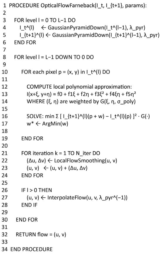
Figure 5. Pseudocode for optical flow (Farnebäck method), applied in this research, where the asterisk (*) denotes the optimal value obtained by minimization.

4. Case Study

Figure 6 shows a wide map of the Bednja River and its global position [52].

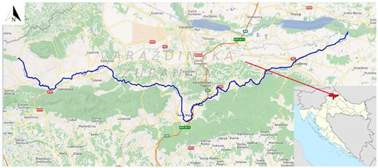
Figure 6. The blue line indicates the course of the Bednja River, while the red arrow marks the location of the study area within Varaždin County, Croatia.

The Bednja River is the right tributary of the Drava River, which springs from smaller streams at an elevation of 300 m and maintains a constant flow at the foot of Macelj, near Brezova Gora in the northwest part of Croatia. It should be emphasized that the Bednja is the longest river in Croatia with a source and estuary in the same country [53]. Figure 7 shows the water catchment with the tributaries of the Bednja River [53,54]. The Bednja flows into the Drava River near Mali Bukovec (at an elevation of 136 m) and is 133 km long, with a basin area of 596 km² [55]. In the Bednja basin, three relief units stand out: alluvial plain, tertiary mountains, and Paleozoic mountains.

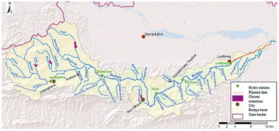
Figure 7. Water catchment of Bednja River.

The characteristics of the Bednja River include its buoyant (variable) flow, increased flow during more intense precipitation events, and the possibility of a drastic reduction in flow during summer [56].

Figure 8 shows the microlocation of the analyzed locations.

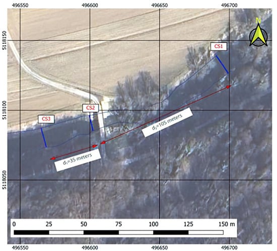
Figure 8. Microlocation of the analyzed site: blue arrows indicate the positions of the measured cross profiles (CS1–CS3), red double-headed arrows indicate the distances between cross profiles, and the labeled values denote the corresponding spacing.

The direction of the river flow is from CS3 to CS1. The bottom of the watercourse consists of gravel and sand, mixed with silt (mud). The banks of the river are overgrown with grass, low bushes, and trees.

5. Results and Discussion

Fieldwork was conducted on 18 April 2025. The depth profiles and maximum surface velocities for the specified cross profiles (CS1, CS2, and CS3) were obtained using three different methods: mobile phone measurements, UAV-based measurements, and PCM measurements. The data collected during the field surveys are presented in the following figures, illustrating the results of measurements conducted at the specified cross profiles. Figure 9, Figure 10, Figure 11, Figure 12, Figure 13, Figure 14, Figure 15, Figure 16 and Figure 17 present the results for cross profiles CS1, CS2, and CS3 obtained using PCM, UAV-based, and mobile phone measurements. The figures include depth profiles, surface velocity fields, and distributions of maximum surface velocities across the channel width. Figure 9, Figure 12 and Figure 15 collectively present the depth profiles and surface velocity distributions for cross profiles CS1, CS2, and CS3. The depth profiles (a) illustrate the channel morphology at each cross-section, while the associated distributions of maximum surface velocities (b) were obtained from PCM measurements. Figure 10, Figure 13 and Figure 16 collectively present UAV-derived velocity fields for cross profiles CS1, CS2, and CS3. Each figure includes the aerial layout of the measured surface velocities (a) and the associated distribution of maximum surface velocities across the channel width (b). Figure 11, Figure 14 and Figure 17 collectively present mobile-phone-derived velocity fields for cross profiles CS1, CS2, and CS3, showing the measured surface velocities (a) and the corresponding distributions of maximum surface velocities across the channel width (b).

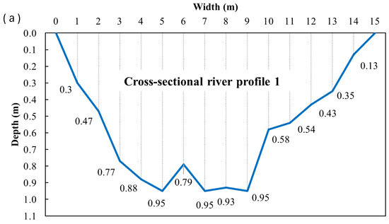
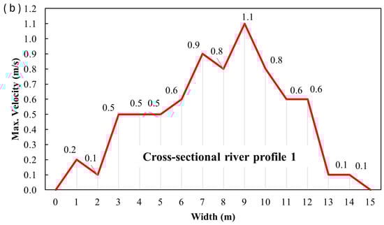
Figure 9. Depth profiles (a) and maximum velocity profiles (b) for cross profile CS1.

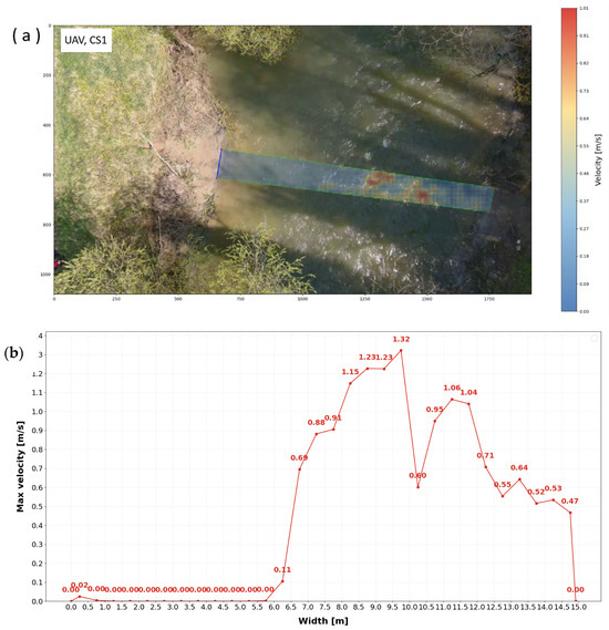
Figure 10. Air layout of maximum velocities obtained by UAV (a), together with distribution of velocities (b) for cross profile CS1.

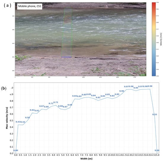
Figure 11. Air layout of velocities obtained by mobile phone (a), together with distribution of maximum velocities (b) for cross profile CS1.

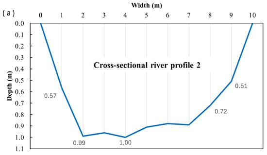
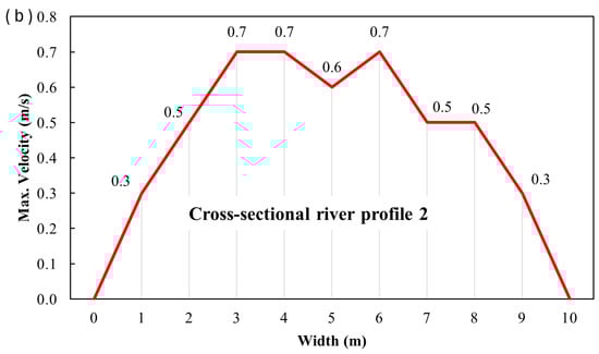
Figure 12. Depth profiles (a) and maximum velocity profiles (b) for cross profile CS2.

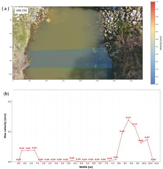
Figure 13. Air layout of velocities obtained by UAV (a), together with distribution of velocities (b) for cross profile CS2.

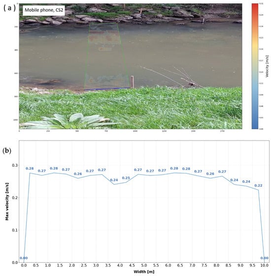
Figure 14. Air layout of velocities obtained by mobile phone (a), together with distribution of velocities (b) for cross profile CS2.

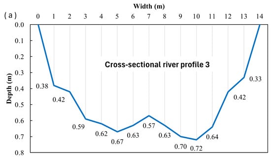
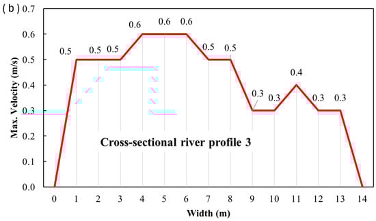
Figure 15. Depth profiles (a) and maximum velocity profiles (b) for cross profile CS3.

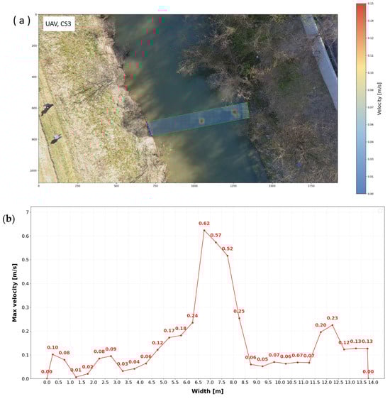
Figure 16. Air layout of velocities obtained by UAV (a), together with distribution of velocities (b) for cross profile CS3.

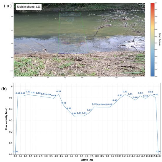
Figure 17. Air layout of velocities obtained by mobile phone (a), together with distribution of velocities (b) for cross profile CS3.

The UAV was flown at the lowest practical altitude, which allowed the camera to capture the entire width in focus. Color changes indicate changes in maximum velocity at the water surface (Figure 10a, Figure 13a and Figure 16a). It is worth noting that, since the ratio of river width to flow depth exceeds 5, the channel can be classified as wide. Consequently, secondary-current effects are weak, and the velocity dip phenomenon, namely the downward shift of the maximum velocity from the free surface, is negligible [57,58]. At the cross profiles CS1 and CS3, the water flow exhibits undulations and a rough water surface. Profile CS2 was calmer, as indicated above.

It should be noted that the minor differences in the maximum velocity values occur at CS1 and CS3, whereas the CS2 profile shows larger differences. As observed, the water face at CS2 has been calmer, i.e., with slight movement.

To provide a first-order comparison between the measurement approaches, Table 1 summarizes the spatially averaged maximum surface velocities obtained from the Propeller Current Meter, UAV, and mobile phone for each cross-section. The absolute differences (Δ) indicate the agreement between the mean velocities derived from different methods. While these values characterize the overall flow magnitude, they do not account for point-wise variations within the velocity profiles, which are addressed by the statistical metrics presented in Table 2.

Table 1. Mean surface velocities and differences between methods in m/s.

Cross Profile	UAV (U)	Mobile (M)	Propeller (P)	ΔU–P	ΔP–M	ΔM–U
CS1	0.46	0.72	0.46	0.01	0.26	0.26
CS2	0.03	0.24	0.44	0.41	0.20	0.21
CS3	0.15	0.43	0.39	0.25	0.04	0.29

Table 2. Statistical comparison between UAV, mobile phone, and propeller measurements.

CS	n	UAV _RMSE	UAV _MAE	UAV _Bias	UAV _R2	UAV _NSE	Mobile _RMSE	Mobile _MAE	Mobile _Bias	Mobile _R2	Mobile _NSE
CS1	16	0.50	0.41	−0.12	0.08	−1.30	0.33	0.24	0.13	0.27	−0.02
CS2	11	0.75	0.66	−0.65	0.19	−3.47	0.53	0.46	−0.46	0.82	−1.25
CS3	15	0.42	0.35	−0.35	0.10	−2.47	0.18	0.16	−0.09	0.51	0.35
ALL	42	0.55	0.46	−0.34	0.02	−2.12	0.36	0.27	−0.10	0.12	−0.31

Although the mean velocities in Table 1 provide a useful first-order comparison between the measurement approaches, they do not reflect the spatial distribution of velocities across the channel. Local deviations between methods may compensate each other when averaged, leading to small mean differences even when point-wise discrepancies are large. Therefore, a point-wise statistical validation was performed by interpolating UAV and mobile phone velocities to the propeller measurement locations and computing standard error metrics.

The statistical agreement between the methods was quantified using the root mean square error (RMSE), mean absolute error (MAE), bias, coefficient of determination (R²), and Nash–Sutcliffe efficiency (NSE), as summarized in Table 2.

Table 2 shows that the mobile phone approach consistently yields lower RMSE and generally higher NSE values than the UAV across all cross-sections, indicating more robust overall agreement with the Propeller Current Meter. For CS1, characterized by higher velocities and increased surface turbulence, UAV-derived velocities reproduce the location and magnitude of the velocity maximum in the flow core; however, larger deviations occur near the channel margins, resulting in a relatively high RMSE and a negative NSE. In CS2 and to a lesser extent in CS3, calmer flow conditions and reduced surface texture lead to larger errors in UAV-based estimates, whereas the presence of floating natural tracers in mobile phone recordings improves velocity detection.

Mean agreement is best for UAV vs. propeller in CS1 (ΔU–P≈0), and for mobile vs. propeller in CS3 (ΔP–M = 0.04). The mobile phone shows the lowest absolute differences relative to the Propeller Current Meter when mean values are considered. However, these averages do not describe how velocities vary across the channel.

This behavior is mainly related to the sensitivity of optical flow methods to surface texture. In turbulent conditions, the water surface contains visible structures, such as ripples and bubbles, that can be tracked in UAV images. In calmer conditions, such as in CS2 and to a lesser extent in CS3, the surface becomes smoother and less structured, leading to larger local errors and a marked drop in NSE for the UAV.

These errors are additionally influenced by small UAV motions during hovering and by minor camera or gimbal adjustments, which introduce small frame-to-frame shifts in the video. In CS2 and CS3, floating natural material (e.g., leaves) in mobile phone videos served as tracers, increasing surface texture and helping the optical flow algorithm yield more stable velocity estimates than those from UAV footage of a relatively smooth water surface.

Scatter plots and Bland–Altman diagrams were prepared for all three cross-sections (CS1–CS3) to support the statistics reported in Table 2. In the scatter plots, points represent paired values at the propeller sampling locations (Propeller on the x-axis; UAV or Mobile on the y-axis). The black diagonal line indicates the 1:1 relationship (perfect agreement), while the blue line shows the fitted linear regression with a 95% confidence band. The Bland–Altman plots display the differences between methods relative to their means.

Figure 18 illustrates the results for CS1. The mobile phone shows a stronger relationship with the propeller measurements than the UAV, with RMSE = 0.333 m/s and R² = 0.267, compared to the UAV (RMSE = 0.501 m/s, R² = 0.079). The UAV differences are more dispersed, with values approaching −1 m/s, consistent with the negative bias (−0.122 m/s) and the poor NSE (−1.303). The mobile phone differences are more tightly grouped, with a smaller bias (0.126 m/s) and an NSE close to zero (−0.018), indicating greater stability in agreement with the propeller measurements for this cross-section.

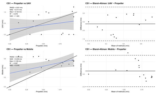
Figure 18. CS1 comparison with Propeller Current Meter: scatter plots (left) and Bland–Altman diagrams (right) for UAV (top) and mobile phone (bottom).

For CS2, the agreement with the propeller measurements is weaker than in CS1, as shown by both the scatter plots and the error statistics (Figure 19, Table 2). The UAV shows very large point-wise errors, with an RMSE of 0.75 m/s and a strongly negative NSE of −3.47, indicating poor agreement with the reference data. The relationship with the propeller measurements is weak (R² = 0.19), and the Bland–Altman plot shows wide differences, with a tendency to underestimate velocities, especially at medium and higher flow speeds. The mobile phone performs better in this cross-section. Its RMSE of 0.53 m/s is clearly lower than that of the UAV, and the R² of 0.82 shows that it captures the spatial variability of velocities across the profile more consistently. However, the NSE remains negative (−1.25), indicating that the absolute errors remain considerable. This is also visible in the Bland–Altman plot, where the differences are more compact than for the UAV but remain biased. These results are consistent with the hydraulic conditions in CS2. Flow velocities are relatively low, and the water surface is smooth, providing little texture for optical flow tracking. Under these conditions, UAV-based estimates degrade more strongly, whereas the mobile phone benefits from floating natural tracers and image stabilization, which improve motion detection and lead to better agreement with the propeller measurements.

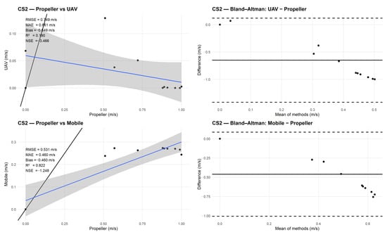
Figure 19. CS2 comparison with Propeller Current Meter: scatter plots (left) and Bland–Altman diagrams (right) for UAV (top) and mobile phone (bottom).

Figure 20 illustrates the results for CS3. The UAV shows weak agreement with the propeller measurements, with an RMSE of 0.42 m/s, a low coefficient of determination (R² = 0.10), and a strongly negative NSE of −2.47 (Table 2), indicating poor point-wise agreement. This is also visible in the Bland–Altman plot, where the UAV differences are widely scattered and reach values below −0.7 m/s, reflecting a general underestimation of velocities. The mobile phone performs noticeably better in this cross-section. It has a lower RMSE of 0.18 m/s, a higher R² of 0.51, and a positive NSE of 0.35 (Table 2), showing that it reproduces both the magnitude and the spatial variability of surface velocities more reliably than the UAV. In the Bland–Altman plot, most differences in mobile phone speed are within ±0.3 m/s and are clustered around zero. This behavior is consistent with the flow conditions in CS3, where moderate velocities and the presence of floating natural material provide sufficient surface texture for the mobile phone recordings, while the smoother surface and small platform motions reduce the reliability of UAV-based optical flow estimates.

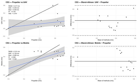
Figure 20. CS3 comparison with Propeller Current Meter: scatter plots (left) and Bland–Altman diagrams (right) for UAV (top) and mobile phone (bottom).

6. Conclusions

This study shows that surface flow velocities can be derived from UAV and smartphone videos and that these approaches are useful when direct measurements in a river are difficult or unsafe, such as during high water levels or flood events.

The results indicate that the performance of image-based methods depends strongly on flow conditions and on the amount of visible structure on the water surface. UAV recordings give the best results when the flow is faster and more turbulent, as in CS1, where the position and magnitude of the maximum velocity in the channel center are reproduced reasonably well. In such conditions, the nadir viewing geometry limits geometric distortions and provides sufficient surface features for optical flow tracking. In calmer flows, however, the smoother water surface and small platform motions lead to larger errors in the UAV-derived velocities.

The smartphone method proved to be more stable across all three cross-sections. It generally produced lower errors and better agreement with the propeller measurements, especially under calmer flow conditions. This can be attributed to optical image stabilization and to the presence of floating natural material, such as leaves, which helps to make surface motion easier to detect in the video.

Overall, the proposed approach offers a practical way to estimate surface velocities from video data, with clear limitations related to flow conditions and recording quality. UAV and smartphone measurements should therefore be regarded as complementary: UAVs perform best in faster, more turbulent flows, while smartphones tend to be more reliable in smoother water surfaces.

References

- Bahmanpouri, F.; Eltner, A.; Barbetta, S.; Bertalan, L.; Moramarco, T. Estimating the Average River Cross-Section Velocity by Observing Only One Surface Velocity Value and Calibrating the Entropic Parameter. Water Resour. Res. 2022, 58, e2021WR031821. [Google Scholar] [CrossRef]
- Zhang, Z.-W.; Zou, Z.-L. Application of Power Law to Vertical Distribution of Longshore Currents. Water Sci. Eng. 2019, 12, 79–86. [Google Scholar] [CrossRef]
- Brauneck, J.; Gattung, T.; Jüpner, R. Surface Flow Velocity Measurements from UAV-Based Videos. Int. Arch. Photogramm. Remote Sens. Spatial Inf. Sci. 2019, 42, 221–226. [Google Scholar] [CrossRef]
- Kinzel, P.J.; Legleiter, C.J. sUAS-Based Remote Sensing of River Discharge Using Thermal Particle Image Velocimetry and Bathymetric Lidar. Remote Sens. 2019, 11, 2317. [Google Scholar] [CrossRef]
- Zhou, Z.; Riis-Klinkvort, L.; Jørgensen, E.A.; Haugård Olesen, D.; Rietz Vesterhauge, A.; Coppo Frías, M.; Lavish, M.; Nielsen, S.; Gustafsson, D.; Wennerberg, D.; et al. UAS Hydrometry: Contactless River Water Level, Bathymetry, and Flow Velocity—The Rönne River Dataset. Sci. Data 2025, 12, 294. [Google Scholar] [CrossRef]
- Torres, W.; Torres, A.; Valencia, E.; Pinchao, P.; Escobar-Segovia, K.; Cando, E. Experimental Validation of the Remote Sensing Method for River Velocity Measurement Using an Open-Source PIV Scheme—Case Study: Antisana River in the Ecuadorian Andes. Water 2024, 16, 3177. [Google Scholar] [CrossRef]
- Tauro, F.; Arcangeletti, E.; Petroselli, A. Assessment of Drone-Based Surface Flow Observations. Hydrol. Process. 2015, 29, 5393–5405. [Google Scholar] [CrossRef]
- Liu, W.-C.; Lu, C.-H.; Huang, W.-C. Large-Scale Particle Image Velocimetry to Measure Streamflow from Videos Recorded from Unmanned Aerial Vehicle and Fixed Imaging System. Remote Sens. 2021, 13, 2661. [Google Scholar] [CrossRef]
- Eltner, A.; Sardemann, H.; Grundmann, J. Technical Note: Flow Velocity and Discharge Measurement in Rivers Using Terrestrial and Unmanned-Aerial-Vehicle Imagery. Hydrol. Earth Syst. Sci. 2020, 24, 1429–1445. [Google Scholar] [CrossRef]
- Fujita, I.; Notoya, Y.; Shimono, M. Development of UAV-Based River Surface Velocity Measurement by STIV Based on High-Accurate Image Stabilization Techniques. In Proceedings of the 36th IAHR World Congress, The Hague, The Netherlands, 28 June–3 July 2015. [Google Scholar]
- Yu, K.; Lee, J. Method for Measuring the Surface Velocity Field of a River Using Images Acquired by a Moving Drone. Water 2023, 15, 53. [Google Scholar] [CrossRef]
- Kriščiūnas, A.; Čalnerytė, D.; Akstinas, V.; Meilutytė-Lukauskienė, D.; Gurjažkaitė, K.; Barauskas, R. Framework for UAV-Based River Flow Velocity Determination Employing Optical Recognition. Int. J. Appl. Earth Obs. Geoinf. 2024, 134, 104154. [Google Scholar] [CrossRef]
- Barnum, P.; Hu, B.; Brown, C. Exploring the Practical Limits of Optical Flow; Technical Report No. 806; Computer Science Department, University of Rochester: Rochester, NY, USA, 2003. [Google Scholar]
- Alfarano, A.; Maiano, L.; Papa, L.; Amerini, I. Estimating Optical Flow: A Comprehensive Review of the State of the Art. Comput. Vis. Image Underst. 2024, 249, 104160. [Google Scholar] [CrossRef]
- Jyoti, J.S.; Medeiros, H.; Sebo, S.; McDonald, W.M. River velocity measurements using optical flow algorithm and unoccupied aerial vehicles: A case study. Flow Meas. Instrum. 2023, 91, 102341. [Google Scholar] [CrossRef]
- La Salandra, M.; Colacicco, R.; Panza, S.; Fumai, G.; Dellino, P.; Capolongo, D. RivAIr: A Custom-Designed UAV-Based Sensor for Real-Time Water Area Segmentation and Surface Velocity Estimation. Int. J. Appl. Earth Obs. Geoinf. 2025, 142, 104720. [Google Scholar] [CrossRef]
- Lou, H.; Zhang, Y.; Yang, S.; Wang, X.; Pan, Z.; Luo, Y. A New Method for Long-Term River Discharge Estimation of Small- and Medium-Scale Rivers by Using Multisource Remote Sensing and RSHS: Application and Validation. Remote Sens. 2022, 14, 1798. [Google Scholar] [CrossRef]
- Eltner, A.; Mader, D.; Szopos, N.; Nagy, B.; Grundmann, J.; Bertalan, L. Using Thermal and RGB UAV Imagery to Measure Surface Flow Velocities of Rivers. Int. Arch. Photogramm. Remote Sens. Spatial Inf. Sci. 2021, XLIII-B2-2021, 717–722. [Google Scholar] [CrossRef]
- Ochoa-García, S.A.; Massó, L.; Patalano, A.; Matovelle-Bustos, C.M.; Delgado-Garzón, P.V. Baseflow Measurement in Mountain Rivers Using LSPIV. Rev. Teledetec. 2025, 66, 227–233. [Google Scholar] [CrossRef]
- Koutalakis, P.; Stamataki, M.-D.; Tzoraki, O. Enhancing the monitoring protocols of intermittent flow rivers with UAV-based optical methods to estimate the river flow and evaluate their environmental status. Drones Auton. Veh. 2024, 1, 10006. [Google Scholar] [CrossRef]
- Zhang, E.; Zhang, X.; Li, X. A Rapid Measurement Method of Surface Flow Velocity Based on Unmanned Aerial Vehicle. SSRN 2024. [Google Scholar] [CrossRef]
- Masafu, C.; Williams, R.; Shi, X.; Yuan, Q.; Trigg, M. Unpiloted Aerial Vehicle (UAV) Image Velocimetry for Validation of Two-Dimensional Hydraulic Model Simulations. J. Hydrol. 2022, 612, 128217. [Google Scholar] [CrossRef]
- Wolff, F.; Lotsari, E.; Spieler, D.; Elias, M.; Eltner, A. Enhancement of Two-Dimensional Hydrodynamic Modelling Based on UAV-Flow Velocity Data. Earth Surf. Process. Landf. 2024, 49, 2736–2750. [Google Scholar] [CrossRef]
- Biggs, H.; Smart, G.; Doyle, M.; Eickelberg, N.; Aberle, J.; Randall, M.; Detert, M. Surface Velocity to Depth-Averaged Velocity—A Review of Methods to Estimate Alpha and Remaining Challenges. Water 2023, 15, 3711. [Google Scholar] [CrossRef]
- Westerberg, I.; Mansanarez, V.; Lyon, S.; Lam, N. Rapid Streamflow Monitoring with Drones. In Proceedings of the EGU General Assembly 2023, EGU23-12058, Vienna, Austria, 23–28 April 2023. [Google Scholar] [CrossRef]
- Chen, M.; Chen, H.; Wu, Z.; Huang, Y.; Zhou, N.; Xu, C.-Y. A Review on the Video-Based River Discharge Measurement Technique. Sensors 2024, 24, 4655. [Google Scholar] [CrossRef] [PubMed]
- Yu, K.; Hwang, J. Development of a Real-Time Surface Image Velocimeter Using an Android Smartphone. J. Korea Water Resour. Assoc. 2016, 49, 469–480. [Google Scholar] [CrossRef][Green Version]
- Yuan, Y.; Che, G.; Wang, C.; Yang, X.; Wang, J. River Video Flow Measurement Algorithm with Space-Time Image Fusion of Object Tracking and Statistical Characteristics. Meas. Sci. Technol. 2024, 35, 055301. [Google Scholar] [CrossRef]
- Dramais, G.; Le Coz, J.; Camenen, B.; Hauet, A. Advantages of a Mobile LSPIV Method for Measuring Flood Discharges and Improving Stage–Discharge Curves. J. Hydro-Environ. Res. 2011, 5, 301–312. [Google Scholar] [CrossRef]
- Jodeau, M.; Hauet, A.; Paquier, A.; Le Coz, J.; Dramais, G. Application and Evaluation of LS-PIV Technique for the Monitoring of River Surface Velocities in High Flow Conditions. Flow Meas. Instrum. 2008, 19, 117–127. [Google Scholar] [CrossRef]
- Cheng, X.; Zhang, X. Image Processing Techniques for Dynamic Surface Velocity Measurement in Rivers. Trait. Signal 2024, 41, 363–372. [Google Scholar] [CrossRef]
- Hu, Q.; Wang, J.; Zhang, G.; Jianhui, J. Space-Time Image Velocimetry Based on Improved MobileNetV2. Electronics 2023, 12, 399. [Google Scholar] [CrossRef]
- Szupiany, R.N.; Amsler, M.L.; Parsons, D.R.; Best, J. Morphology, Flow Structure, and Suspended Bed Sediment Transport at Two Large Braid-Bar Confluences. Water Resour. Res. 2009, 45, e2337. [Google Scholar] [CrossRef]
- Blanckaert, K.; Duarte, A.P.C.; Chen, Q.; Schleiss, A. Flow Processes near Smooth and Rough (Concave) Outer Banks in Curved Open Channels. J. Geophys. Res. Earth Surf. 2012, 117, 4020. [Google Scholar] [CrossRef]
- Dodangeh, E.; Afzalimehr, H. Incipient Motion of Sediment Particles in the Presence of Bed Forms under Decelerating and Accelerating Flows. J. Hydrol. Hydromech. 2022, 70, 89–102. [Google Scholar] [CrossRef]
- Yang, T.; Liu, Z.; Chen, Y.; Yu, Y. Real-Time, Inexpensive, and Portable Measurement of Water Surface Velocity through Smartphone. Water 2020, 12, 3358. [Google Scholar] [CrossRef]
- Damtie, M.T.; Jumber, M.B.; Zimale, F.A.; Tilahun, S.A. Assessment of a Smartphone App for Open Channel Flow Measurement in Data-Scarce Irrigation Schemes. Hydrology 2023, 10, 22. [Google Scholar] [CrossRef]
- Carrel, M.; Detert, M.; Peña-Haro, S.; Lüthi, B. Evaluation of the DischargeApp: A Smartphone Application for Discharge Measurements. In Proceedings of the HydroSenSoft International Symposium on Hydro-Environment Sensors and Software, Madrid, Spain, 26 February–1 March 2019. [Google Scholar]
- Lüthi, B.; Philippe, T.; Peña-Haro, S. Mobile Device App for Small Open-Channel Flow Measurement. In Proceedings of the 7th International Congress on Environmental Modelling and Software (iEMSs 2014), San Diego, CA, USA, 15–19 June 2014. [Google Scholar]
- Peña-Haro, S.; Lüthi, B.; Philippe, T. A Smartphone App for Measuring River Discharge. In Proceedings of the EGU General Assembly Abstracts, Vienna, Austria, 8–13 April 2018. [Google Scholar]
- Knaak, J.; Oberleithner, K.; Paschereit, C.O. SmartPIV: Flow Velocity Estimates by Smartphones for Education and Field Studies. Exp. Fluids 2021, 62, 242. [Google Scholar] [CrossRef]
- Perks, M.T.; Dal Sasso, S.F.; Hauet, A.; Jamieson, E.; Le Coz, J.; Pearce, S.; Peña-Haro, S.; Pizarro, A.; Strelnikova, D.; Tauro, F.; et al. Towards Harmonisation of Image Velocimetry Techniques for River Surface Velocity Observations. Earth Syst. Sci. Data 2020, 12, 1545–1559. [Google Scholar] [CrossRef]
- Bonacci, O. Utvrđivanje količina vode koje poniru na dionicama vodotoka u kršu. Naš Krš 1981, VI, 139–151. [Google Scholar]
- Puliti, S.; Solberg, S.; Granhus, A. Use of UAV Photogrammetric Data for Estimation of Biophysical Properties in Forest Stands under Regeneration. Remote Sens. 2019, 11, 233. [Google Scholar] [CrossRef]
- Castro, A.I.; Shi, Y.; Maja, J.M.; Peña, J.M. UAVs for Vegetation Monitoring: Overview and Recent Scientific Contributions. Remote Sens. 2021, 13, 2139. [Google Scholar] [CrossRef]
- Krause, S.; Sanders, T.; Mund, J.; Greve, K. UAV-Based Photogrammetric Tree Height Measurement for Intensive Forest Monitoring. Remote Sens. 2019, 11, 758. [Google Scholar] [CrossRef]
- Taddia, Y.; González, L.; Zambello, E.; Pellegrinelli, A. Quality Assessment of Photogrammetric Models for Façade and Building Reconstruction Using DJI Phantom 4 RTK. Remote Sens. 2020, 12, 3144. [Google Scholar] [CrossRef]
- Chen, S.; McDermid, G.J.; Castilla, G.; Linke, J. Measuring Vegetation Height in Linear Disturbances in the Boreal Forest with UAV Photogrammetry. Remote Sens. 2017, 9, 1257. [Google Scholar] [CrossRef]
- Ridolfi, E.; Manciola, P. Water Level Measurements from Drones: A Pilot Case Study at a Dam Site. Water 2018, 10, 297. [Google Scholar] [CrossRef]
- Fakhri, S.A.; Motayyeb, S.; Saadatseresht, M.; Zakeri, H.; Mousavi, V. Comparison of UAV Image Spatial Resolution Based on the Siemens Star Target. ISPRS Ann. Photogramm. Remote Sens. Spat. Inf. Sci. 2022, 10, 143–149. [Google Scholar] [CrossRef]
- Farnebäck, G. Two-Frame Motion Estimation Based on Polynomial Expansion. In Image Analysis; Bigün, J., Gustavsson, T., Eds.; Springer: Berlin/Heidelberg, Germany, 2003; Volume 2749, pp. 363–370. [Google Scholar] [CrossRef]
- Google Maps. Available online: https://www.google.com/maps/place/Bednja (accessed on 26 October 2022).
- Đurin, B.; Plantak, L.; Bonacci, O.; Di Nunno, F. A Unique Approach to Hydrological Behavior along the Bednja River (Croatia) Watercourse. Water 2023, 15, 589. [Google Scholar] [CrossRef]
- Croatian Waters. Studija Utjecaja na Okoliš za EU Projekt Zaštite od Poplava na Slivu Bednje: Netehnički sažetak. 2018. Available online: https://www.bednja.hr/media/1598.pdf (accessed on 18 January 2026).
- Petrić, H. On Some Settlements in the River Bednja River Basin during the Middle Ages and at the Beginning of the Early New Age. Kaj Časopis Književnost Umjet. Kult. 2010, 43, 91–116. [Google Scholar]
- Ðurin, B.; Kranjčić, N.; Muhar, A.M. Smart Hydro-Energy Hybrid System Potential in Croatia—Bednja River Case Study. Electron. J. Fac. Civ. Eng. Osijek—E-GFOS 2020, 11, 39–50. [Google Scholar]
- Yang, S.Q.; Tan, S.K.; Lim, S.Y. Velocity distribution and dip-phenomenon in smooth uniform open channel flows. J. Hydraul. Eng. 2004, 130, 1179–1186. [Google Scholar] [CrossRef]
- Rezazadeh, S.; Manafpour, M.; Bahmanpouri, F.; Gualtieri, C. Application of the entropy model to estimate flow discharge and bed load transport in a large river. Phys. Fluids 2025, 37, 3684. [Google Scholar] [CrossRef]
Disclaimer/Publisher’s Note: The statements, opinions and data contained in all publications are solely those of the individual author(s) and contributor(s) and not of MDPI and/or the editor(s). MDPI and/or the editor(s) disclaim responsibility for any injury to people or property resulting from any ideas, methods, instructions or products referred to in the content. |
© 2026 by the authors. Licensee MDPI, Basel, Switzerland. This article is an open access article distributed under the terms and conditions of the Creative Commons Attribution (CC BY) license.