Multivariate Analysis and Hydrogeochemical Evolution of Groundwater in a Geologically Controlled Aquifer System: A Case Study in North Central Province, Sri Lanka

Abstract

This study investigates the coupled relationship between groundwater chemistry, lithology, and structural features in the dry zone of Netiyagama, Sri Lanka, within a fractured crystalline basement. Groundwater chemistry fundamentally reflects geological conditions determined by rock-water interactions, we hypothesized that the specific spatial patterns of groundwater chemistry in heterogeneous fractured systems are distinctly controlled by integrated effects of lithological variations, structurally driven flow pathways, aquifer stratification, and geochemical processes, including cation exchange and mineral-specific weathering. To test this, we integrated hydrogeochemical signatures with mapped hydrogeological data and applied multi-stage multivariate analyses, including Piper diagrams, Hierarchical Cluster Analysis (HCA), and Principal Component Analysis (PCA), and various bivariate plots. Piper diagrams identified five distinct hydrochemical facies, but these did not correlate directly with specific rock types, highlighting the limitations of traditional methods in heterogeneous settings. Employing a multi-stage multivariate analysis, we identified seven clusters (C1–C7) that exhibited unique spatial distributions across different rock types and provided a more refined classification of groundwater chemistries. These clusters align with a three-unit aquifer framework (shallow weathered zone, intermittent fracture zone at ~80–100 m MSL, and deeper persistent fractures) controlled by a regional syncline and lineaments. Further analysis through bivariate diagrams revealed insights into dominant weathering processes, cation-exchange mechanisms, and groundwater residence times across the identified clusters. Recharge-type clusters (C1, C2, C5) reflect plagioclase-dominated weathering and short flow paths; transitional clusters (C3, C7) show mixed sources and increasing exchange; evolved clusters (C4, C6) exhibit higher mineralization and longer residence. Overall, the integrated workflow (facies plots + PCA/HCA + bivariate/process diagrams) constrains aquifer dynamics, recharge pathways, and flow-path evolution without additional drilling, and provides practical guidance for well siting and treatment.

1. Introduction

The association between groundwater chemistry and lithology in dry zones is an essential topic in hydrogeology. The geological features of the domain are one of several variables that affect the chemistry of groundwater. In fractured crystalline terrains, groundwater composition is primarily shaped by processes such as mineral dissolution–precipitation, cation exchange, and redox reactions, which vary with residence time and fracture connectivity [1,2]. Understanding the link between groundwater chemistry, lithology, and structures is significant for sustainable water management and resource planning in arid and semi-arid zones, where water resources are frequently scattered and vulnerable [3,4]. Because recharge is limited and circulation is slow, dry-zone aquifers often develop high mineralization and spatial heterogeneity due to prolonged water–rock contact [5].

The sorts of minerals that are found in the subsurface depend on the lithology of a region. Groundwater may experience a number of chemical reactions that affect its composition as it interacts with these minerals. For example, certain minerals can release ions into the groundwater, changing its physical and chemical qualities [4,6]. In Sri Lanka’s dry zone, these processes operate within Precambrian crystalline aquifers of the Wanni and Highland complexes, where silicate-weathering signatures and cation exchange reactions have been documented [7,8].

In crystalline-rock aquifers, permeability depends primarily on the density and connectivity of fractures, as only a minority of these structures are hydraulically active [9]. Such heterogeneity produces strong spatial variations in groundwater chemistry even within a single lithology [10]. To identify various water bodies and define groundwater systems, hydrogeochemical investigations in fractured crystalline rock commonly use major and minor dissolved ions. However, to unravel overlapping geochemical influences, multivariate statistical tools such as Principal Component Analysis (PCA) and Hierarchical Cluster Analysis (HCA) are increasingly used alongside conventional graphical methods [2,11]. In this study, we hypothesize that groundwater chemistry reflects distinct geological conditions controlled by lithological and structural variability, and that even within a single lithology, differences in fracture connectivity, mineralogy, and residence time result in variable water–rock interactions.

The study area, Netiyagama, is a dry-zone village located in the Anuradhapura District of Sri Lanka’s North Central Province, where groundwater occurs in fractured crystalline aquifers. Previous investigations have shown that groundwater in this region is generally neutral to slightly alkaline, with elevated total dissolved solids (TDS) and significant concentrations of silica, strontium, and chloride, features that indicate strong silicate weathering and extended residence time in the aquifers [7,8,12]. Based on the literature, the geochemistry of groundwater in this area indicates a strong influence of rock–water interactions, with major ions derived mainly from feldspars, amphiboles, and other silicate minerals in the underlying metamorphic formations Nevertheless, most existing studies have emphasized chemical classification and provenance, with limited integration of structural geology and subsurface heterogeneity, which are critical for understanding groundwater evolution [13].

Globally, fractured crystalline aquifers are characterized by strong mineralization and wide geochemical variability between shallow and deep systems, reflecting prolonged residence times and lithological control [10,14]. Similar patterns have been recognized in Sri Lankan basement aquifers [8].

The objective of this study is to integrate hydrogeochemical signatures with hydrogeological and geological data to improve understanding of the subsurface framework without relying solely on costly drilling operations. Specifically, the study aims to (i) characterize groundwater facies using Piper and Gibbs diagrams; (ii) apply PCA and HCA to identify statistically distinct groundwater groups; (iii) relate these clusters to lithological and structural domains; and (iv) infer dominant hydrogeochemical processes such as silicate weathering, ion exchange, and mixing. This integration aims to use hydrogeochemical mapping to delineate aquifers, recharge zones, and groundwater flow paths, thereby improving conceptual models of groundwater evolution and resource sustainability. To test the hypothesis, the study combines geological and structural field observations with chemical datasets through a multi-stage multivariate workflow. Conventional Piper diagrams provide first-order hydrochemical facies classification, while HCA and PCA reveal finer distinctions linked to lithology and structure [2,11]. In crystalline terrains such as Netiyagama, this integrated approach provides a more robust understanding of aquifer heterogeneity than any single classification method.

2. Materials and Methods

2.1. Study Area

2.1.1. Geological Setting of the Study Area

The study area was selected with the specific intention of supporting the establishment of a water treatment plant for a resource-limited school situated in the Anuradhapura-Mihintale region, a dry zone village (Netiyagama) located in the North Central Province of Sri Lanka. This locale was chosen deliberately because it is situated at the central point of the study region, ensuring that the hydrological assessments and subsequent water supply interventions are directly beneficial to the school community. To adequately characterize the groundwater and surface water resources relevant to this project, a representative part of a basin covering the Netiyagama area, which includes the school area, was delineated.

This region is characterized by relatively flat terrain, with elevations ranging ≈ 90–140 m. It is traversed by branches of the Aruvi Aru (Malwathu Oya) and Mahakanadara Ala, forming part of the Malwathu Oya basin. The headwaters of the Mahakanadarawa and Aruvi Aru are located in the southeastern portion of the study area. Both of these channels converge into the Mahakanadarawa tank, which has a total holding capacity of 36,250 acre-feet (equivalent to 44,713,717 cubic meters). This tank is formed by damming the Kanadarawa Oya, the primary tributary of the Malwathu Oya. The area has a 75 percent expectancy of >775 mm rainfall a year, with most rainfall from the northeast monsoon between December and February [15].

2.1.2. Geological and Hydrogeological History of Sri Lanka

High-grade metamorphic Basement formation of Sri Lanka is considered a Neoproterozoic event, which happened during the Neoproterozoic Gondwana collision with the closure of the Mozambique Ocean due to the collision of east and west Gondwana lands. Based on geological, structural, mineralogical, and petrological evidence, the Sri Lankan basement is composed of four distinctly different crustal blocks resulting from the amalgamation of Gondwana in the Pan-African orogeny. These blocks are known as the Wanni Complex (WC), the Highland Complex (HC) and the Vijayan Complex (VC), and the Kadugannawa Complex [16,17]. About nine-tenths of the island is underlain by these Proterozoic high-grade rocks. The study region geologically belongs to the Wanni Complex, the westernmost crustal block in Sri Lanka, which consists of a variety of metaigneous rocks and metasediments

The geological evolution of the island fundamentally controls the hydrogeological history and long-term climatic conditions. The crystalline basement rocks are composed of negligible primary porosity. Therefore, groundwater systems developed mainly through secondary porosity generated by tectonic fracturing and deep tropical weathering [18,19]. Prolonged subaerial exposure promoted intense chemical weathering under tropical climatic conditions, leading to the formation of regolith profiles over large parts of the island (Figure 1). These weathered zones, together with fracture networks in the underlying bedrock, became the principal groundwater reservoirs in the crystalline terrains [7]. Recharge to these aquifers has been historically controlled by monsoonal rainfall patterns, resulting in strong spatial and temporal variability in groundwater availability and chemistry.

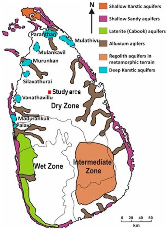
Figure 1. Different types of aquifers in Sri Lanka (Modified after [18]).

A major hydrogeological differentiation occurred during the Middle Miocene, when marine transgressions affected the northern and northwestern parts of Sri Lanka, leading to the deposition of Miocene limestone formations, particularly in the Jaffna Peninsula [20]. These carbonate deposits subsequently evolved into highly productive karstic aquifers with high transmissivity and storage capacity. In contrast, the central and southern regions of Sri Lanka, including the mid-country crystalline terrains, remained emergent during the Miocene and were not subjected to marine sedimentation. From the Late Miocene to Quaternary periods, climatic oscillations and sea-level fluctuations further influenced groundwater development. In coastal and alluvial settings, Quaternary sea-level changes affected shallow aquifer geometry and salinity distribution, particularly in low-lying coastal plains [18].

2.1.3. Hydrogeology of Fractured Hard-Rock Aquifers

In the Precambrian metamorphic terrain, groundwater is hosted within fractured hard-rock aquifers characterized by negligible primary porosity and total dependence on secondary fracture porosity for storage and transmission [21]. These aquifers function as dual-porosity systems, consisting of a shallow weathered regolith zone (saprolite) and a deeper fractured bedrock zone, each exhibiting distinct hydrogeological properties, recharge dynamics, and implications for groundwater salinity.

Shallow Weathered Zone, also known as Regolith Aquifer, typically has depths ranging from 5 to 30 m and rarely exceeding 40 m in thicker profiles. This aquifer consists of clay-dominated saprolite produced through intense chemical weathering of underlying Precambrian gneisses, charnockites, and quartzites under tropical climatic conditions, resulting in a porous but low-permeability layer [22]. Despite high total porosity (10–30%), hydraulic conductivity is severely limited due to the clay-rich matrix, positioning the regolith primarily as a storage reservoir with restricted transmissivity rather than a conduit for lateral flow [18,22]. Recharge occurs directly and rapidly during monsoon periods (northeast: December–February; southwest: May–September), making the aquifer highly responsive to rainfall variability and prone to seasonal depletion during inter-monsoon dry spells. Yields are low to moderate (0.1–2 L/s), sufficient to sustain traditional dug wells and shallow agro-wells widely used for domestic supply and small-scale irrigation in rural Dry Zone communities [18].

The Deep Fractured Bedrock Aquifer underlies the regolith across Sri Lanka’s Dry Zone, extending from >25 m to over 150 m in productive zones, with groundwater flow along fracture networks potentially reaching >300 m in structural depressions such as synformal keels or along the HC-VC thrust boundary [18,21] aquifer comprises fresh to slightly altered crystalline bedrock of the Highland Complex (HC), Vijayan Complex (VC), and Wanni Complex (WC) (Figure 2a), dominated by granitic gneisses, charnockitic gneisses, and migmatites formed during Proterozoic sedimentation (~2.0 Ga) and Pan-African high-grade metamorphism (~610–455 Ma [22]. Primary porosity is near zero (<0.5%), rendering the rock matrix effectively impermeable; all effective porosity and permeability are secondary, governed by fracture density, aperture, orientation, and interconnectivity within deformation-generated networks [21]. Recharge is slow and indirect, occurring via percolation through the overlying regolith or along major fracture conduits, and is severely restricted by the arid climate, low matrix permeability, and limited flushing in flat topography [23].

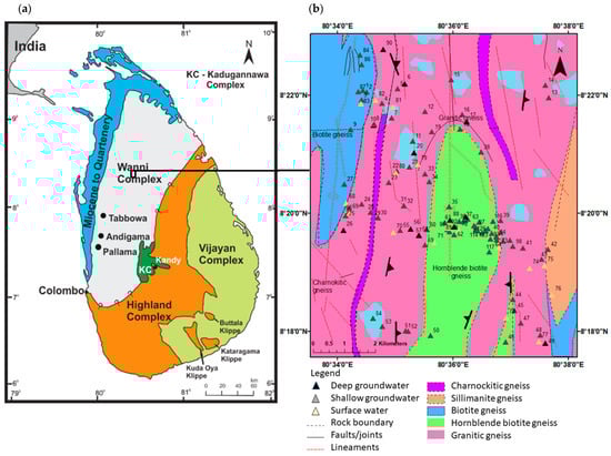
Figure 2. (a) Geological map of Sri Lanka with lithological units indicated by color codes (as shown in the figure); (b) geology of the study area showing sampling locations, where numbers denote sample labels.

2.1.4. Lithological and Structural Pattern Distribution of the Study Area

The 1:100,000 scale geological maps provide detailed geological information covering the entirety of Sri Lanka, divided into a series of sheets. This scale offers a balance between detailed representation and coverage extent, making the maps highly useful for various scientific, educational, and practical applications. The series is published by the Geological Survey and Mines Bureau of Sri Lanka, a government authority responsible for geological surveying, mapping, and mineral resource evaluation throughout the country. 1:100,000 geological maps of 8-Anuradhapura-Polonnaruwa and 6 A-Vavuniya-Trincomalee were used for the lithological study of the area.

However, reliance on 1:100,000 scale maps introduce certain uncertainties, particularly when applied to large-scale research such as hydrogeochemical analysis in a geologically controlled aquifer system. These maps, while effective for regional overviews, are inherently small-scale representations that generalize lithological boundaries to accommodate broader geographic coverage. As a result, boundaries between rock units may be depicted with lower precision, potentially oversimplifying complex transitions, fault lines, or subtle variations in lithology that occur at finer scales. For instance, the mapped edges of formations like hornblende biotite gneiss or charnockite layers could be approximate, leading to uncertainties in delineating aquifer boundaries, recharge zones, or groundwater flow paths. Such generalizations might not capture micro-scale heterogeneities, such as localized fracturing or weathering patterns, which are critical for accurate hydrogeological modeling. To mitigate these limitations, we supplemented map interpretation with ground-truthing (field validation), GPS-based structural measurements, and lineament analysis from satellite imagery, following best practice for fractured-rock terrains [21].

The study area is surrounded by thick, though tectonically repeated sequences of orthogneisses with a complex history of charnockitization, retrogression, and local re-charnockitization, which hampers easy recognition of the protoliths. Five major types of Proterozoic metamorphic rocks are exposed in the area of concern (Figure 2b). The majority of the area, including headwaters, represents granites and flows across thick bodies of hornblende biotite gneiss. Layers of charnockite can be identified as minor occurrences along the flow path. Downstream areas are dominated by biotite gneiss with minor occurrences of charnockite and pegmatite layers (1:100,000 geological map, sheet 8). Granitic gneiss, which is dominantly found within the area, can be identified as massive leucocratic quartzo-feldspathic gneisses with quartz > 20% and few mafic minerals. The second predominant rock type, hornblende biotite gneiss, is identified as massive to compositionally layered grey gneiss with quartz > 20%, plagioclase and garnet < 10%, and a tonalite composition. The biotite gneiss is massive or compositionally layered, pale grey gneiss which contains quartz, feldspar, and >10% biotite, generally granodioritic to quartz-monzonitic in composition. Often, ridge-forming restricted outcrops of charnockitic gneisses are typically coarse-grained with characteristic brown or green greasy luster; they may lack hypersthene. Garnetiferous quartz-feldspar gneiss are leucocratic quartz-feldspar gneiss with abundant pink garnets > 20% that weather to iron-rich residual deposits. Distinctive quartz-rich leucocratic white or pink pegmatite layered gneisses in the area are usually produced by ridge-forming processes [22,24,25]. These units correspond to the Wanni-Complex crystalline basement and are consistent with regional syntheses [22].

2.1.5. Regional Groundwater Salinity Indicators

Electrical conductivity (EC) and total dissolved solids (TDS), which offer a direct measurement of the total ionic content in water, are the two main physical indicators of groundwater salinity (Figure 3). Since EC measures the capacity of water to conduct electricity, which rises with the concentration of dissolved salts, it is frequently employed as a quick and accurate stand-in for salinity. TDS, either measured directly or estimated from EC, represents the total mass of dissolved ions and complements EC in quantifying salinity levels.

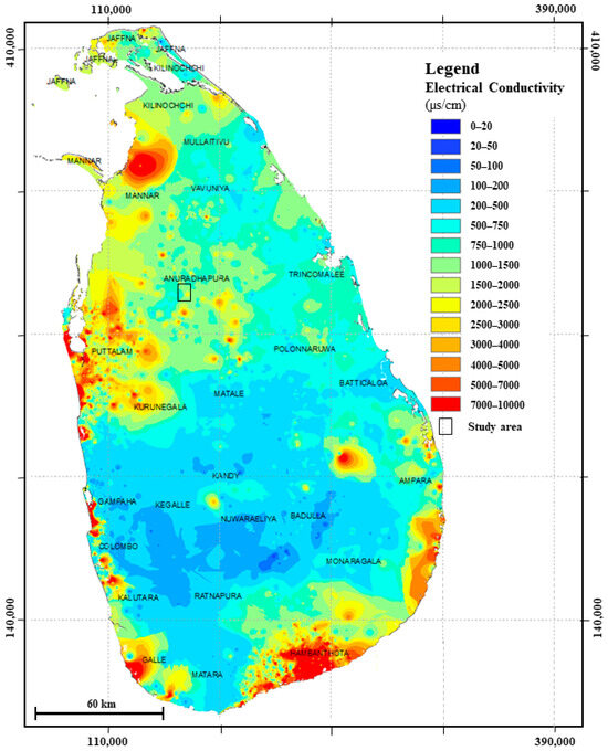
Figure 3. Regional map of the Electrical conductivity variation of groundwater modified after [26].

Rock samples of hornblende biotite gneiss, biotite gneiss, charnockitic gneiss, and granitic gneiss were collected for petrological and mineralogical studies, representing the geological diversity of the study area.

2.2. Water Sampling and Rock Sampling

Water samples analyzed for geochemistry include 98 from shallow wells, 16 from surface water, and 16 from deep wells. Shallow groundwater samples were collected from dug wells (~8 m), while deep groundwater samples were obtained from tube wells (>25 m). The sampling process was carried out across the study area, and the GPS coordinates of the locations were recorded using a Global Positioning System (GPS) receiver. Water samples were collected into properly labeled high-density polyethylene (HDPE) bottles, which were acid-soaked overnight and then washed thoroughly with deionized water before being oven-dried. Before filling, each bottle was rinsed three times with site water. In situ measurements of pH, temperature, electrical conductivity (EC), and total dissolved solids (TDS) were made using a calibrated multiparameter meter. Alkalinity was determined in the laboratory using an auto-titrator.

2.3. Analytical Procedure

Total alkalinity, pH, and TDS and EC were measured with the field meter and cross-checked in the laboratory for each unfiltered raw sample within 24 h of collection. Samples were pressure-filtered through 0.22 µm filters, and filtered samples were analyzed for anions by Ion Chromatography (IC) and for cations through Inductively Coupled Plasma Optical Emission Spectroscopy (ICP-OES). All water chemical analyses were performed at the National Institute of Fundamental Studies, Sri Lanka.

Thin sections were prepared from the collected rock samples, and detailed optical analyses were conducted using a polarizing microscope at the Department of Geology, University of Peradeniya. This enabled a comprehensive evaluation of their mineralogical and textural characteristics.

2.4. Hydrogeochemical Analysis

Collected physicochemical data were used to investigate hydrochemical facies using Piper trilinear diagrams [27]. The basic statistical analysis was done for the samples using OriginPro 2024 and R (v4.3.3). Before multivariate analysis, variables were inspected for outliers and skew; log-transformation was applied where appropriate, and all variables were standardized to z-scores [28]. Gibbs plots were created to examine dominant geochemical controls (precipitation, evaporation, rock–water interaction) [29]. 1:100,000 geological maps (Anuradhapura-Polonnaruwa and Vavuniya-Trincomalee) provided by Geological Survey and Mines Bureau (GSMB) were used to create the geological map of the study area, and the Inverse Distance Weighting (IDW) spatial analysis tool in ArcGIS 10.8 and 30 m SRTM DEM (with Google Earth Pro used for visualization and field navigation) were used for the preparation of spatial distribution maps of hydrogeochemical facies as well as to create the Digital Elevation Model (DEM) map of the area. IDW surfaces were evaluated with leave-one-out cross-validation; root-mean-square error (RMSE) values and prediction–observation plots indicated acceptable performance for descriptive mapping [30]. Both DEM map and hydrochemical facies maps and plots were used to determine evolutionary trends of groundwater.

2.5. Software Tools and Platforms

2.5.1. Water Clustering

The standardized dataset was initially utilized to perform Piper classification using OriginPro 2024 to identify and categorize the various water types, thereby determining the predominant water type within the study area. Following this, Principal Component Analysis (PCA) was conducted to identify and select key elements that characterize specific water types. This selection was based on mineral reactions and trace elements derived from the weathering of minerals within the lithology of the region, effectively linking water chemistry with geological features. The PCA results enabled the identification of trace and minor elements essential for further analysis. Subsequently, Hierarchical Cluster Analysis (HCA) was performed using the R programming environment, applying the Euclidean distance metric combined with Ward’s clustering method, which is well-suited for geology-related cluster analyses due to its ability to minimize variance within clusters efficiently [31]. Retention of principal components followed the Kaiser criterion (eigenvalues > 1) and cumulative variance (>70%) [28]. HCA dendrogram stability was assessed by varying linkage distance cut-offs. This comprehensive approach allowed for a robust classification and interpretation of the hydrochemical data, enhancing the understanding of groundwater characteristics and their controlling factors [2].

2.5.2. Geospatial Analysis

Geospatial distribution maps illustrating the hydrogeochemical signatures were generated using the Inverse Distance Weighted (IDW) interpolation method, a spatial analyst tool implemented within ArcGIS version 10.8. This methodology enabled the spatial visualization and assessment of groundwater chemistry variations across the area of interest. Additionally, Digital Elevation Models (DEM) were constructed to capture topographical features impacting groundwater flow and quality; elevation data were sourced from 30 m SRTM; Google Earth Pro assisted visual validation and field referencing. The integration of geospatial tools facilitated the detection of spatial patterns and potential zones of contamination or resource vulnerability, thereby providing critical insights for water resource management and planning [29,31].

2.5.3. Geochemical Processes Analysis

The clusters obtained from the hierarchical cluster analysis were subsequently plotted on Gibbs diagrams and bivariate plots to elucidate the dominant geochemical processes affecting groundwater quality and the evolutionary trends of groundwater clusters in the study region. These graphical tools provide a framework to interpret processes such as precipitation dominance, rock-water interaction, and evaporation effects on water chemistry. The combined use of these geochemical analyses serves to deepen the understanding of groundwater evolution and its controlling natural processes within the geological context of the study area.

3. Results and Discussion

3.1. Aquifer Characterization and Hydrogeological Setting

Geological maps and structural measurements indicate that the majority of the sampling points are located in a zone exhibiting structural characteristics of a syncline (Figure 4a). A set of well log data within the study area was selected to define the aquifer in this specific zone. In folded crystalline terrains, fracture density and transmissivity commonly increase along fold axes, favouring local storage and focused flow; thus, synformal geometry can strongly influence groundwater occurrence and chemistry [21,32].

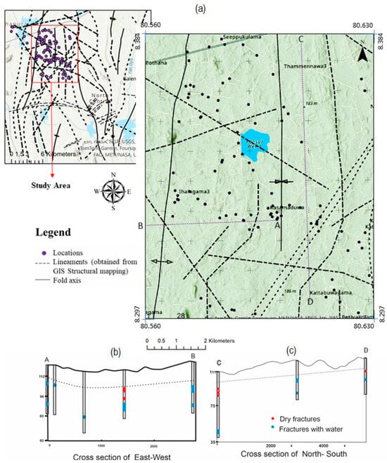
Figure 4. (a) Map showing the groundwater flow direction and all lineaments, including possible weak zones, around the study area; (b) AB cross-section; (c) CD cross-section created for fracture conditions study.

Two cross sections were constructed across the study area (Figure 4b,c); one extending from east to west and another from northwest to southeast. The cross sections cover a substantial portion of the study area and were created to investigate fracture patterns and aquifer setting. According to the well logs obtained from the National Water Supply and Drainage Board, hard rock was encountered at depths ranging from 9.5 m to 15.5 m below the surface, with an average overburden thickness of 10–12 m. In certain areas, shallow well water levels occur as deep as ~8 m below the surface. The depth of the wells considered for the aquifer study ranged from 36 m to 72 m. The Netiyagama school well, which lies on the syncline axis, shows more fractures compared to other well logs, consistent with the tendency for higher fracture intensity along fold axes [21]. Deeper fractures (>25 m) showed considerable groundwater yield, but the majority of small fractures were dry. In contrast, other well logs reveal that wells located away from the syncline axis contain shallow fractures with better groundwater yield, demonstrating the influence of the syncline structure on fracture distribution. The yield data indicate that the groundwater extraction wells utilized to produce cross sections range from 0 to 40 L per minute. Upon analyzing the groundwater production data from the tube wells in the study area, the greatest yield recorded was 60 L per minute. The availability of groundwater from deep fractures increased from northwest to southwest and from east to west.

Three major aquifers were delineated using the field data and well logs. The first is a shallow, unconfined aquifer that most of the shallow dug wells. Beneath this unconfined shallow aquifer lies a hard rock interval with sparse fracturing. A zone of water-bearing fractures (80–100 m MSL) was identified below that layer from well logs, which could serve as a confined or semi-confined aquifer. The fractures in the shallow hard rock layers may be discontinuous, as some fractures are dry. This suggests the potential presence of isolated pockets of perched water within the shallow levels (~15 m) of weathered rock. In contrast, deeper levels of hard rock (below 80 m MSL) contain another set of fractures that are continuous and water-bearing, according to the well logs. This deeper fractured zone can function as a confined aquifer layer based on the available data. Vertical compartmentalization of weathered regolith, discontinuous shallow fractures, and deeper persistent fracture zones is typical of basement terrains [21,32,33]. These three distinct aquifer layers are expected to have distinct water chemistry. As water is extracted from all three layers, their mixing could cause alteration of water quality. Consequently, bulk well chemistry may not resolve the water chemistry of each aquifer layer without depth-specific sampling [34].

3.2. Groundwater Flow Patterns of the Study Area

The analysis of groundwater flow patterns indicates significant interactions between geological features and hydrological dynamics. As illustrated in Figure 4, the faulting and lineament orientations predominantly trending north–south (NS), northwest-southeast (NW–SE), and west–east (W–E) direct groundwater movement towards the Mahakanadarawa tank. This directional flow is consistent correlation between groundwater depth and altitude, with shallower depths observed at lower elevations. Notably, regions exhibiting elevated nitrate concentrations are associated with reduced groundwater levels, highlighting susceptibility to anthropogenic influences. Such patterns are common where shallow flow paths intersect cultivated or settled areas and where hydraulic gradients towards surface-water bodies enhance exchange during wet periods [34,35]. Occasional elevated nitrate in deeper samples may reflect vertical connectivity via fractures or well construction effects; confirmation would require depth-discrete sampling and tracers [35].

3.3. Major Ion Chemistry

A statistical comparison of the regional distribution of water-quality parameters is shown in Table 1. Within-group variability was evaluated using the coefficient of variation (CV, %), which aids interpretation of heterogeneity across water types [36]. Descriptive statistics for the three water types show that pH values are generally near neutral, with shallow waters tending to be slightly higher than deep and surface waters. This may reflect higher evaporation under dry conditions and enhanced dissolution/alkalinity generation from water–rock interaction in the weathered zone [1,34].

Table 1. Major Chemical constituents of water.

Parameter	Shallow					Deep					Surface
	Mean	Min	Median	Max	CV	Mean	Min	Median	Max	CV	Mean	Min	Median	Max	CV
pH	7.38	6.45	7.40	8.18	0.066	7.17	6.40	7.25	8.06	0.064	7.37	6.56	7.40	8.57	0.064
EC (μS/cm)	686.70	150.00	634.50	1450.00	0.473	754.38	300.00	729.00	1850.00	0.635	419.43	124.40	460.00	650.00	0.437
TDS (mg/L)	344.02	75.00	325.00	725.00	0.044	320.80	369.00	390.00	1035.00	0.701	280.49	83.30	308.00	435.00	0.474
Na+ (mg/L)	76.74	15.46	60.88	317.22	0.785	74.17	22.06	52.47	159.46	0.610	46.94	14.09	56.59	78.95	0.480
K+ (mg/L)	5.29	0.52	2.28	26.14	1.181	4.59	2.07	3.99	9.72	0.515	5.64	3.19	4.73	7.25	0.215
Ca2+(mg/L)	74.79	14.51	74.23	230.05	0.541	63.73	18.08	54.72	169.32	0.707	21.40	6.67	18.13	90.64	0.857
Mg2+ (mg/L)	7.36	0.04	0.04	31.88	0.622	6.37	0.01	0.04	56.71	0.511	0.04	2.89	0.01	5.93	1.081
Cl− (mg/L)	125.19	0.00	78.52	668.23	0.081	124.72	21.94	78.35	308.40	0.701	83.81	10.86	81.34	152.18	0.552
NO3− (mg/L)	8.38	0.01	0.94	86.08	2.020	37.46	0.04	4.39	243.21	1.965	3.08	0.06	1.43	26.69	2.001
SO42− (mg/L)	45.75	8.21	37.19	193.58	0.699	48.78	18.38	45.82	78.74	0.418	18.81	0.05	19.37	39.44	0.434
HCO3− (mg/L)	268.17	10.01	229.56	734.10	0.450	250.80	22.41	263.63	564.32	0.664	112.07	37.06	118.36	200.86	0.408
CO32− (mg/L)	24.40	0.49	22.32	73.74	0.867	25.60	1.10	26.52	56.70	0.699	11.40	3.72	11.94	20.22	0.388
Si (mg/L)	43.27	14.19	46.36	62.82	0.303	52.41	34.43	54.22	70.90	0.203	6.17	3.53	5.87	11.19	0.314

Shallow groundwater indicates the highest electrical conductivity (~687 μS/cm) and total dissolved solids (~345 mg/L), consistent with moderate mineralization from extended contact with weathered regolith. Deep groundwater EC and TDS exceed surface-water values, as expected for longer residence times and more extensive water–rock interaction. TDS concentrations ranged in shallow water from ~75 to ~725 mg/L and in deep water from ~369 to ~1035 mg/L, showing high variability across groups.

Compared to deep and surface waters, shallow waters have high concentrations of major ions such as Na⁺, K⁺, Ca²⁺, Mg²⁺, Cl⁻, and HCO₃⁻, as well as total hardness (TH) and total alkalinity (TA), indicating stronger near-surface water–rock interaction. While surface-water measurements show less fluctuation, both shallow and deep groundwater exhibit significant nitrate with high variability (mean 8.38 and 37.46 mg/L, respectively; surface water ~3.08 mg/L). Because nitrate is reactive and source-dependent, these values should be interpreted with land-use context [35]. Trace contributions to hardness from Sr, Fe, and Mn (Table 2) are typically minor; however, elevated Sr variability is consistent with the weathering of plagioclase and biotite in granitic–gneiss terrains [1].

Table 2. Minor and Trace elements variation over the study area.

Element	Shallow			Deep			Surface
	N Total	Mean (meq/L)	CV	N Total	Mean (meq/L)	CV	N Total	Mean (meq/L)	CV
Mn	81	0.00208	5.918	15	0.00289	2.221	17	3.81 × 10−4	1.808
Co	71	1.68 × 10−5	0.458	12	1.81 × 10−5	0.126	16	1.86 × 10−5	0.142
Cu	75	6.13 × 10−5	3.564	13	1.21 × 10−4	2.090	16	3.62 × 10−5	0.000
Zn	75	2.18 × 10−4	1.889	12	6.11 × 10−4	1.417	16	2.74 × 10−4	0.855
Cd	70	1.56 × 10−5	0.344	12	1.58 × 10−5	0.358	16	1.13 × 10−5	0.111
Al	64	4.51 × 10−4	2.188	13	1.93 × 10−4	1.121	17	0.00149	0.701
B	64	0.02033	0.549	13	0.01721	0.383	17	0.02158	0.752
Pb	81	0.7408	4.414	15	7.41 × 10−5	0.272	17	0.88238	4.123
As	73	5.16 × 10−4	0.522	12	4.99 × 10−4	0.523	16	5.19 × 10−4	0.208
Ni	57	7.41 × 10−6	0.250	10	7.17 × 10−6	0.000	17	3.52 × 10−5	0.692
Sr	81	0.01532	0.656	15	0.01558	0.576	17	0.00471	0.584
Cs	36	0.00165	0.699	7	0.00202	0.603	16	0.00255	0.442
Ba	64	0.0038	0.515	13	0.00336	0.714	17	0.00109	0.574
Bi	57	1.50 × 10−4	0.000	10	1.50 × 10−4	0.000	16	1.50 × 10−4	0.000
Ag	57	3.98 × 10−5	0.388	10	3.92 × 10−5	0.367	16	4.27 × 10−5	0.075
Ga	57	8.46 × 10−4	0.000	10	8.46 × 10−4	0.000	16	8.46 × 10−4	0.000
Li	64	4.78 × 10−4	0.879	13	0.00138	1.128	17	2.65 × 10−5	0.593
Cr	57	4.50 × 10−5	0.000	10	4.50 × 10−5	0.000	16	4.50 × 10−5	0.000
Fe	64	2.57 × 10−4	1.348	13	2.17 × 10−4	1.341	17	0.00256	1.213

Note: N, Number of Samples; CV, Coefficient of Variation.

CV indicates that shallow water is more variable in Na⁺, K⁺, Cl⁻, NO₃⁻, SO₄²⁻, and Mg²⁺, whereas surface water shows greater sensitivity in TH and Ca²⁺. Deep water exhibits higher variability in TDS, alkalinity, and HCO₃⁻, reflecting residence-time effects. Across all samples, HCO₃⁻, TH, TA, Na⁺, and Ca²⁺ exert the strongest influence on bulk hydrogeochemistry. Dissolved silica (as SiO₂), Sr, Fe, SO₄²⁻, NO₃⁻, and Cl⁻ also vary considerably despite moderate means. The mass-abundance order for dissolved species is HCO₃⁻ > Cl⁻ > Na⁺ > Ca²⁺ > SO₄²⁻ > Mg²⁺ >SiO₂ > NO₃⁻ > K⁺ in shallow water and HCO₃⁻ > Cl⁻ > Na⁺ > Ca²⁺ > SO₄²⁻ > Mg²⁺ >SiO₂ > K⁺ > NO₃⁻ in deep water, while surface water shows HCO₃⁻ > Cl⁻ > Na⁺ > Ca²⁺ > SO₄²⁻ > Mg²⁺ > K⁺ > NO₃⁻ > SiO₂.

3.4. Minor and Trace Ion Chemistry

The coefficient of variation (CV) and mean concentrations of trace elements across shallow, deep, and surface waters indicate distinct geochemical behaviour and sources. Elements such as Mn, Pb, Cu, and Al show high variability (CV > 2) in shallow and surface waters, suggesting heterogeneity driven by redox fluctuations, mineral dissolution/precipitation, adsorption–desorption, and potential anthropogenic inputs [34]. Moderately variable species (e.g., Zn, Fe, Li) in deep water likely reflect lithology-controlled variation and longer residence times. In contrast, elements such as Co, Cd, Ni, Sr, Cs, Ba, As, Ag, and B exhibit low variability, indicating uniform geogenic control and effective buffering. Elements at or below detection limits (e.g., Bi, Ga, Cr in this dataset) exhibit negligible variance. Shallow waters display high variability in Mn, Cu, Pb, and Al, likely due to active interaction with soils and fluctuating Eh–pH conditions; surface waters show elevated and variable Pb, Mn, Al, and Fe, potentially influenced by runoff and suspended particulates. Sr appears diagnostic for water-type differentiation, consistent with plagioclase weathering in the gneissic host rocks [37].

3.5. Piper Classification

The Piper diagram analysis reveals five hydrochemical facies across groundwater (both deep and shallow) and surface water The most dominant water type is Ca–HCO₃, primarily located within zone 1 of the central diamond field (region A–E), consistent with recent recharge and short flow paths. The Na–Cl type (zone 2; region D–G) reflects salinity enrichment that may arise from evapoconcentration, ion exchange, or dissolution of residual salts; marine mixing is unlikely inland and should not be inferred without supporting evidence [1,33]. In this dataset, most Na–Cl samples correspond to surface waters. The mixed Ca–Mg–Cl type (zone 3; cation region B, anion region G) suggests mixing and longer residence-time interaction with the rock matrix. The Ca–Na–HCO₃ type (zone 4; cation regions B–D, anion region E) indicates active cation exchange (Na⁺ uptake from clays/altered feldspars balanced by Ca²⁺ release), characteristic of transitional flow fields. Finally, the Ca–Cl facies (zone 5; region A–G) reflects salinity acquisition via evaporative concentration or reverse ion exchange, and can also indicate inputs from deeper mineralized waters; anthropogenic sources (e.g., effluents) are possible but require corollary tracers (e.g., NO₃⁻, B, δ¹⁵N–NO₃⁻) [33].

3.6. Statistical Classification of Water

PCA

Based on CV patterns and mean concentrations, Mn, Pb, Cu, Al, and Fe appear to be the key trace elements contributing to water type differentiation, so we applied Principal Component Analysis (PCA) to quantify which variables drive variance in groundwater [27]. The principal component analysis was conducted independently from the hierarchical cluster analysis on 19 geochemical variables (Si, Fe, Mn, Co, Cu, Zn, Cd, Al, B, Pb, As, Ni, Sr, Ba, Bi, Ag, Ga, Li, Cr). All variables were log-transformed as needed and z-standardized before PCA; components were retained by the Kaiser criterion (eigenvalue > 1) and inspected with the scree plot [28]. The eigenvalues, percentage of variance explained, and cumulative variance for each principal component are summarized in Table 3, while the corresponding scree plot is illustrated in Figure 5.

Table 3. Eigenvalues of the Correlation Matrix.

Eigenvalue	Percentage of Variance	Cumulative
4.25952	22.42%	22.42%
3	15.79%	38.21%
2.45525	12.92%	51.13%
1.80367	9.49%	60.62%
1.25429	6.60%	67.22%
1.22096	6.43%	73.65%
1.04111	5.48%	79.13%
0.81315	4.28%	83.41%
0.77978	4.10%	87.51%
0.57597	3.03%	90.55%
0.54575	2.87%	93.42%
0.39839	2.10%	95.51%
0.32505	1.71%	97.23%
0.21386	1.13%	98.35%
0.15598	0.82%	99.17%
0.11264	0.59%	99.77%
0.04465	0.23%	100.00%

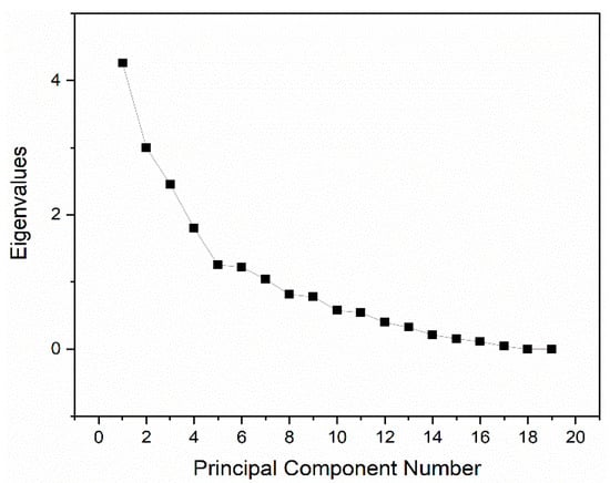
Figure 5. Eigenvalues for principal components.

According to PCA, moderate-to-weak but interpretable loadings with values ≥ 0.30 were highlighted (Table 4). PC1 (22.42% of variance) is characterized by positive loadings of Si, Pb, Cd, and Ba, suggesting coupled silicate weathering (Si) with trace-metal mobilization potentially via adsorption/desorption or particulate association [37]. PC2 (15.79%) is dominated by Bi, Ga, and Cr, pointing to a distinct trace-metal behaviour that may reflect low-level geogenic sources and sorption controls; interpretation should consider detection limits [34]. PC3 (12.92%) shows positive loadings for Zn, Cu, and Ag, consistent with a group of redox- and sorption-sensitive metals [38]. PC4 (9.49%) loads positively on B (and weakly on Ag), which can indicate mixed inputs (detergents/fertilisers for B) and/or differential adsorption; negative loadings for Zn, Cu, As suggest contrasting sources or partitioning [33,37].

Table 4. Extracted Eigenvalues.

	PC1	PC2	PC3	PC4
Mn	0.06368	9.90 × 10−16	0.23758	−0.29224
Co	0.04069	9.17 × 10−15	0.29662	0.28234
Cu	0.05266	2.12 × 10−15	0.3468	−0.31749
Zn	0.03487	2.82 × 10−15	0.45643	−0.4005
Cd	0.36437	1.94 × 10−15	0.27127	0.19941
Al	−0.26404	1.19 × 10−16	0.05608	−0.03213
B	0.08257	3.58 × 10−16	−0.15654	0.35152
Pb	0.41939	7.44 × 10−16	0.05024	0.0376
As	0.02485	−5.48 × 10−15	−0.4458	−0.36854
Ni	−0.29864	1.42 × 10−16	0.03855	0.23955
Sr	0.2949	−1.69 × 10−15	−0.25595	0.10965
Ba	0.31156	−1.37 × 10−15	−0.18881	0.04238
Bi	−4.60 × 10−16	0.57735	−5.78 × 10−15	−2.61 × 10−15
Ag	0.09318	3.91 × 10−15	0.32305	0.41696
Ga	−4.62 × 10−16	0.57735	−5.78 × 10−15	−2.60 × 10−15
Li	0.24577	7.00 × 10−16	0.08903	−0.07738
Cr	−4.62 × 10−16	0.57735	−5.78 × 10−15	−2.60 × 10−15
Si	0.4396	−4.32 × 10−16	−0.06993	−0.10741
Fe	−0.26258	4.02 × 10−16	0.06819	0.09747

The spatial arrangement of variables in the loading plot helps identify which elements drive the separation of samples (Figure 6), while the score plot shows actual sample groupings. In our loadings, Fe–Mn–Co–Al group together, indicating shared redox/sorption control; Zn–Ag–Cd plot apart, implying distinct behaviour; Ba–Sr–Si–Pb²⁺ align with water–rock interaction and residence-time effects [37]. Overall, PCA corroborates that weathering (Si, Sr, Ba) and redox/sorption processes (Fe, Mn, Co, Al; Cu, Zn) jointly structure trace-element variability.

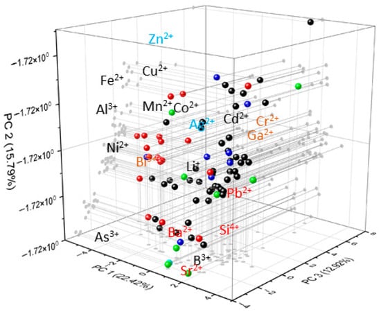
Figure 6. Principal Component Analysis plot illustrating the distribution and behavior of elements along the first three principal components. Different colored points represent the seven clusters identified through hierarchical cluster analysis.

3.7. Hydro-Geochemical Processes and Groundwater Cluster Evolution

3.7.1. Multivariate Analysis Using Litho-Focus Elements

The dominant rock-forming minerals identified in the study area include plagioclase, hornblende, K-feldspar, biotite, quartz, and mafic silicates (e.g., pyroxenes), with accessory magnetite/hematite. The weathering and dissolution of these minerals contribute significantly to groundwater chemistry. Plagioclase (Na–Ca feldspar) releases Na⁺, Ca²⁺, Al³⁺, SiO₂, and Sr²⁺; Sr and Ca are especially diagnostic of plagioclase breakdown [1,36]. K-feldspar, though more resistant, contributes K⁺, Al³⁺, and SiO₂ over longer timescales [39]. Hornblende and other mafic silicates weather to supply Ca²⁺, Mg²⁺, Fe²⁺/Fe³⁺, Al³⁺, SiO₂, and trace metals (e.g., Mn, Zn, Cu, Co), with rates and speciation modulated by pH–Eh conditions [40]. Iron oxides/hydroxides (e.g., goethite/hematite) govern the adsorption–desorption of many trace metals and arsenic [41]. Biotite (K–Fe–Mg mica) weathers relatively rapidly among phyllosilicates, releasing K⁺, Mg²⁺, Fe, Al, Si, and trace metals; it is a key early-stage source of Fe and Mg [38,42,43]. These mineralogical sources justify a lithology-focused variable set for clustering (major ions plus Si, Sr, Fe, Mn, Al, Zn, Cu, Co).

3.7.2. HCA for Litho-Focus Elements and Classified Seven Clusters

This section presents the results of hierarchical cluster analysis (HCA) and geochemical interpretation. Guided by lithology and PCA, we selected major ions (Na⁺, K⁺, Ca²⁺, Mg²⁺, HCO₃⁻, CO₃²⁻, Cl⁻, SO₄²⁻) and lithology-diagnostic species (Si, Sr, Fe, Mn, Al, Zn, Cu, Co) for HCA. HCA was performed using Euclidean distance and Ward’s linkage [2].

Figure 7a shows the dendrogram for 113 groundwater samples; a cut at linkage distance 25 yielded seven clusters (C1–C7), and following the identification of seven clusters through HCA, Stiff diagrams (Figure 7b) were developed to visualize and interpret the major ion distribution patterns associated with each cluster, while piper trilinear diagram was employed to illustrate the distribution of these clusters in terms of hydrochemical facies in Figure 8. We examined cluster stability by varying the cut; formal indices such as silhouette width, cophenetic correlation, or the gap statistic can be used to optimise the number of clusters [44,45].

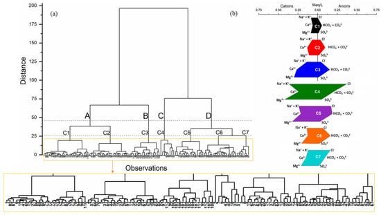
Figure 7. (a) HCA for 113 samples (A–D are the major clusters, and C1–C7 are the subclusters that appeared with the phenon line at 25 distance); (b) stiff diagram for major ion behavior of the derived seven clusters from HCA.

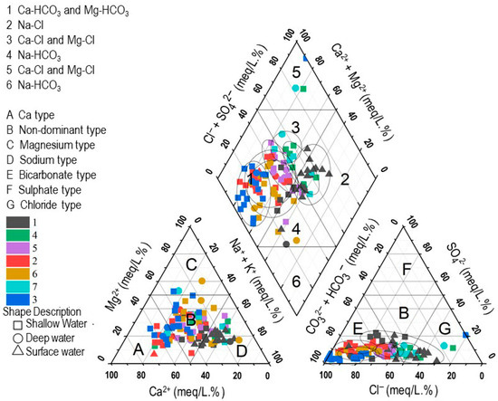
Figure 8. HCA-derived cluster on the piper classification diagram.

To understand geochemical characteristics, box plots of the key parameters for C1–C7 are shown in Figure 9.

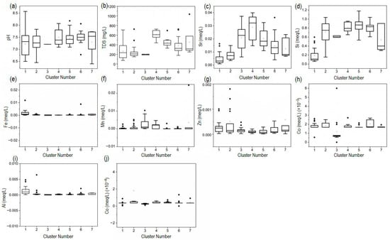
Figure 9. Box-and-whisker plots showing the spatial variation of selected physico-chemical parameters and trace elements across the identified groundwater clusters. Concentrations are expressed in mg/L (TDS) and meq/L for all ions and trace elements, while pH is unitless. Subplots represent: (a) pH, (b) TDS, (c) Sr, (d) Si, (e) Fe, (f) Mn, (g) Zn, (h) Al, (i) Cu, and (j) Co.

C1 is characterized by a wide pH range (~6.5–8.5), elevated Al–Zn with moderate TDS and low Sr–Si, suggesting fresh recharge interacting with aluminosilicates and early-stage ferromagnesian weathering under oxic conditions; minor Fe indicates limited reducing microzones. C2 shows narrower pH (~7.1–7.8), very low Sr, Mn, Al, Cu, moderate Si and low TDS, consistent with near-recharge waters with limited mineralization and possible shallow anthropogenic influence. C3 is near-constant in pH (~7.2) with elevated Sr and moderate Si, occasional Mn spikes, and low Zn–Cu–Al, consistent with more chemically mature flow paths (greater residence time) and stabilised metals. C3–C4 exhibit higher Sr, indicating stronger rock–water interaction (plagioclase weathering). C4–C5 show the highest TDS, indicating more mineralized waters (enhanced interaction and/or evaporative concentration). C4–C7 maintain relatively high, consistent Si, indicating continuing silicate weathering; higher TDS–Sr–Si in C4–C7 suggests longer residence or deeper pathways.

Stiff diagrams highlight spatial/hydrochemical contrasts, cluster-average impression of C1 becomes Na–HCO₃ dominated, with almost all the surface water samples included in C1, while in the piper diagram (Figure 8), the majority of groundwater samples in C1 interpret low mineralization, Ca–HCO₃ dominant, fresh recharge [33]. Only a limited no of C1 groundwater samples are plotted in Na- HCO_3, implying evolved waters with cation exchange [1]. C2 is characterized by relatively balanced contributions of Ca²⁺, Mg²⁺, and Na⁺ + K⁺, with HCO₃⁻ + CO₃²⁻ dominance on the anion side. This indicates a mixed water type, suggesting carbonate dissolution combined with early-stage ion exchange [1]. Cluster C3 displays elevated Na+K⁺ and Mg²⁺, while Ca²⁺ is comparatively lower. Anions are again dominated by HCO₃⁻ + CO₃²⁻, with minor SO₄²⁻ and Cl⁻. This pattern reflects a mixed bicarbonate facies, likely representing evolved groundwater undergoing prolonged water–rock interaction. C4 shows a pronounced Na⁺ + K⁺ dominance among cations, coupled with higher Cl⁻ and SO₄²⁻ concentrations compared to other clusters. This cluster corresponds to a Na-Cl type, indicating salinity enrichment, possibly due to evaporation, anthropogenic inputs, and dissolution of evaporitic or saline minerals. C5: Ca–HCO₃ with minor SO₄²⁻, recharge-like but slightly more evolved than C1. C6: enriched Na⁺ + K⁺ and Cl⁻ with low Ca²⁺/Mg²⁺, suggesting ion-exchange dominated or deep, longer residence water [46]. C7: mixed chemistry (Na⁺ ≈ Ca²⁺, notable Cl⁻/SO₄²⁻), indicative of mixing between recharge and more mineralized sources; potential anthropogenic inputs would require corroborative tracers (e.g., NO₃⁻, B) [1,46]. Consistent with the Piper plot (Figure 8), most groundwater samples plot as Ca–HCO₃ (C1–C3, C5, C6), reflecting recharge-dominated waters controlled primarily by carbonate dissolution and early-stage water–rock interaction. Chloride-dominant facies (C4) indicate chemical evolution via ion exchange/evapoconcentration. C6 spans mixed fields consistent with exchange and deeper weathering. C7 is intermediate, reflecting mixing along convergent flow paths [1,32].

3.7.3. Geology and Cluster Association

C1 occurs mainly in the western sector, over biotite gneiss and granitic gneiss, and extends into the southern granitic gneiss area (Figure 10). This spatial spread across felsic gneisses is consistent with recharge-like Ca–HCO₃ facies in shallow flow paths. C2 spans granitic gneiss and biotite gneiss, with local accumulation within hornblende–biotite gneiss. Most C2 points lie near lineaments and focus toward the mapped syncline, suggesting strong structural control on flow and mixing [21]. C3 is tightly clustered over hornblende–biotite gneiss in the central region, with limited spread into other lithologies, indicating localized hydrochemical control by mafic–intermediate minerals and longer residence along fracture corridors. C4 occurs sparsely in biotite gneiss and eastern granitic gneiss; the limited structural intersection density in this area may reduce focused connectivity. C5, C6, and C7 are widely distributed from southwest to north across hornblende–biotite, granitic, and charnockitic gneisses, consistent with cluster-specific chemistry being governed by both lithology and cross-formational pathways. C5 is often associated with lineaments and represents mixed facies, possibly due to hydraulic connectivity across formations [21].

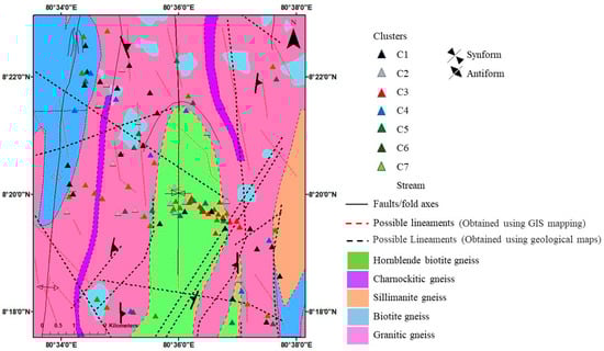
Figure 10. Cluster association with lithology and structures of the area.

C6 shows observable clustering between major antiform and synform traces and is dominated by deeper-aquifer samples, consistent with structurally guided, longer flow paths and enhanced mineralization [20,32].

3.7.4. Combination Diagrams

According to the TDS versus Cl⁻/(Cl⁻ + HCO₃⁻) diagram analysis (Figure 11), the majority of groundwater samples demonstrated Cl⁻/(Cl⁻ + HCO₃⁻) ratios less than 0.5, indicating that HCO₃⁻ concentrations exceeded chloride levels and that rock weathering processes dominated over seawater intrusion contributions [47]. Conversely, only three groundwater clusters displayed Cl⁻/(Cl⁻ + HCO₃⁻) ratios exceeding 0.5, signifying an increasing participation of saline processes, which may include seawater intrusions, anthropogenic inputs, evapo-concentration, and geogenic chloride sources in groundwater composition formation.

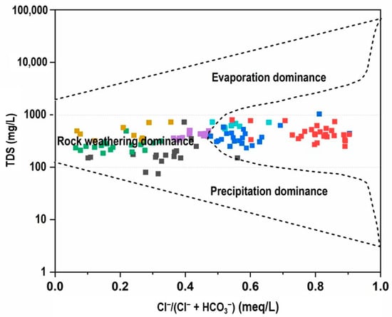
Figure 11. Gibbs plot of TDS vs. Cl⁻/(Cl⁻ + HCO₃⁻) for groundwater samples.

However, seawater intrusion in Sri Lanka is a coastal hydrogeological phenomenon observed in shallow, unconsolidated coastal aquifers and measurable only within a few kilometres of the shoreline [48], thus seawater intrusion is hydrogeologically impossible in the present study area because the aquifer is located far inland with an air distance of ~84 km, within an elevated mid-country crystalline terrain that is fully isolated from coastal groundwater systems (Figure 1). Therefore, the elevated chloride concentrations observed in the dataset must result from non-marine processes, including anthropogenic inputs, rock weathering, and evapoconcentration

The geological context of the study area, characterized by hornblende-biotite gneiss and biotite gneiss, plays a crucial role in explaining the observed salinity patterns. Although chloride-bearing minerals such as biotite and amphibole (Figure 12) contain structurally bound Cl, their weathering under near-surface conditions contributes only minor amounts of chloride when compared with deep crustal brine-forming processes. Reference [49].demonstrated processes that significant chloride release from these minerals occurs primarily in deep, long-residence-time fluid systems, where water-rock interaction persists over millions of years. Such conditions differ fundamentally from the shallow, fractured crystalline aquifers examined in this study. In contrast, several mechanisms relevant to inland hard-rock aquifers more plausibly explain the elevated chloride in clusters C3, C4, and C7. As described by [50], groundwater in crystalline terrains may evolve toward Na–Cl or Cl-rich compositions through a combination of water–rock interaction and cation exchange, localized longer residence time within isolated fractures, and strong evapo-concentration effects during the dry season. Importantly, these processes can generate Cl-rich hydrochemical signatures independent of any marine or coastal influence, and the Na–Cl domain of Gibbs diagrams should not be interpreted as uniquely diagnostic of seawater intrusion.

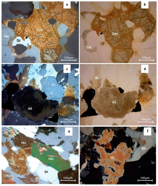
Figure 12. Petrographic thin section analysis under optical microscope under view 5 × 10 × 10; (a,c) Charnockitic gneiss under xpl mode; (b,d) Charnockitic gneiss under ppl mode; (e) Hornblende biotite gneiss under XPL mode; (f) granitic gneiss under xpl mode (Per—perthite; Qz—quartz; Opx—orthopyroxene; Cal—calcite; Bt—biotite; Or—Orthoclase; All—allanite; Hbl—hornblende).

Field evidence from the study area supports this interpretation. Several shallow hard-rock fractures were observed to be discontinuous, with some zones remaining dry, indicating the presence of isolated perched water pockets. Such conditions promote localized groundwater stagnation, enhancing mineral dissolution and enabling chloride accumulation in situ. These observations are fully consistent with the hydrochemical behaviour of inland crystalline aquifers described by [50]. Additional support comes from [51], who documented that soils and weathered regolith in continental environments may accumulate substantial chloride loads, not because they generate chloride internally, but because of atmospheric deposition, evaporation of precipitation, evapotranspiration, and concentration of solutes in shallow groundwater (Figure 13). These processes can produce elevated chloride in shallow aquifers located far from the sea, particularly in tropical regions with strong seasonal drying.

K(Mg, Fe)₃AlSi₃O₁₀(OH, Cl)₂ (Biotite) + 1/2 O₂ + 3H₂O → Al₂Si₂O₅(OH)₄ + K⁺
+ 3 (Mg²⁺, Fe²⁺) + H₄SiO₄ + Cl⁻                    

Ca₂ (Mg, Fe)₄Al(Si₇Al)O₂₂(OH, Cl)₂ (Hornblende) + CO₂ + 5H₂O + 1/2 O₂ →
Al₂Si₂O₅(OH)₄ +2 Ca²⁺ + 4 (Mg²⁺, Fe²⁺) + HCO₃⁻ + H₄SiO₄ +Cl⁻     

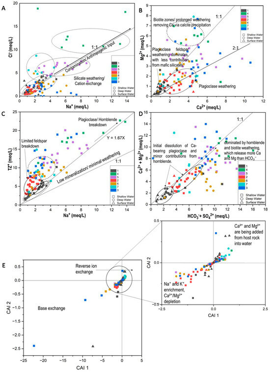
Figure 13. Bivariate diagrams to determine cluster geochemistry; (A) Na vs. Cl; (B) Ca vs. Mg; (C) Na vs. Total Cations; (D) HCO₃⁻ + SO₄₂⁻ vs. Ca + Mg; (E) CAI 1 vs. CAI 2.

A linear Ca vs. Mg trend can indicate co-release from common sources (e.g., dolomite or Mg-bearing silicates), whereas deviations reflect differing contributions and/or secondary processes [1,36]. In this study, C1 exhibits a near-linear distribution along an approximate 2:1 Ca: Mg slope, consistent with a greater Ca contribution from calcic plagioclase and Ca-bearing trace minerals like allanite relative to Mg inputs from mafic silicates, with limited carbonate influence [39,52]. C2 also reflects the dominance of Na–Ca plagioclase weathering and may indicate the influence of cation exchange wherein Na⁺ displaces Ca²⁺ on exchange sites (Figure 13B) [1,53].

CaAl₂Si₂O₈ + H₂CO₃ + 1/2O₂ → Al₂Si₂O₅(OH)₄ + Ca²⁺ + CO₃²⁻
(Anorthite)             (Kaolinite)        

(Ca, Ce, La, Nd, Th)₂(Fe³⁺, Fe²⁺, Ti) (Al, Fe³⁺)₂Si₃O₁₂(OH) (Allanite) + H⁺
+ H₂O → REE³⁺ + Fe³⁺ + Al³⁺ + SiO₂ + Ca²⁺            

NaAlSi₃O₈ → Na⁺ + AlO₂⁻ + 3SiO₂
(Albite)           

In contrast, C4 shows characteristics indicative of more evolved waters (higher residence times), where Ca²⁺ reduction may result from calcite precipitation (Figure 12b) or reverse ion exchange [1,54].

Ca²⁺ + 2 HCO₃⁻ → CaCO₃(s) + CO₂ + H₂O
   (Calcite)

The remaining clusters display a more scattered distribution on the Ca–Mg plot (Figure 13B), suggesting heterogeneous weathering sources and/or mixing along intersecting flow paths [52,54]. For C7, complementary indicators (e.g., NO₃⁻, B, δ¹⁵N–NO₃⁻) would be required to distinguish anthropogenic inputs from exchange-driven signatures [55].

On the Na⁺ vs. TZ⁺ (total cations) diagram (Figure 13C), C2 plots close to the 1:1 line, reflecting low mineralization and early-stage weathering (limited contact time) [51,52]. C3 shows slightly elevated TZ⁺ and Na⁺, indicating moderate weathering and mixed cation sources (Na from albite; Ca–Mg from mafic silicates), typical of transitional flow domains. C4 exhibits the highest Na⁺ and TZ⁺, with points trending along Y ≈ 1.67 X, indicative of advanced silicate weathering and cation exchange that enriches Na⁺ by replacing Ca²⁺/Mg²⁺ on clays [1]. C6 shows broader scatter, implying heterogeneous sources or mixed recharge, consistent with spatial lithologic variability and variable residence times [32,53].

The CAI-1 vs. CAI-2 (Schoeller chloro-alkaline indices) diagram (Figure 13E) shows C2 and C6 predominantly in the negative quadrants, indicating base-exchange softening (Ca²⁺/Mg²⁺ in groundwater replaced by Na⁺ on exchange sites). C4 and C7 lie mostly in the positive quadrants, reflecting reverse ion exchange (Na⁺ in water exchanged for Ca²⁺/Mg²⁺ from the matrix), a pattern typical of salinity enrichment/long residence and occasionally saline intrusion contexts [1,54]. C1 and C5 cluster near zero, suggesting minimal exchange and younger, less-reacted waters. C3 exhibits mixed behaviour consistent with seasonal mixing or lithologic heterogeneity along convergent flow paths.

4. Conclusions

Groundwater chemistry in Netiyagama is jointly controlled by lithology and structure within a fractured crystalline basement. Integrating field hydrogeology, facies plots, multivariate statistics (PCA, HCA), and GIS reveals three hydrostratigraphic units: a shallow unconfined weathered zone, an intermittent fracture zone near ~80–100 m MSL, and deeper persistent fractures, whose connectivity is conditioned by a regional syncline and NS/NW–SE/W–E lineaments. These structures focus transmissivity along fold axes and fracture corridors, producing systematic variations in yield and quality.

Hydrochemically, Ca–HCO₃ waters dominate recent recharge and short flow paths, whereas Na–Cl and mixed facies mark more evolved conditions driven by ion exchange and, locally, evapoconcentration. Shallow groundwater shows the highest EC/TDS and variability, reflecting intense near-surface interaction and land-use influence; deep waters are more stable but have higher TDS than surface water due to longer residence. Variable nitrate in both shallow and deep wells indicate vertical connectivity where structures converge. PCA separates a weathering/residence-time axis (Si, Sr, Ba) from redox/sorption suites (Fe–Mn–Co–Al; Cu–Zn), and HCA resolves seven clusters (C1–C7) that map coherently to lithology and structures: recharge-type Ca–HCO₃ clusters (C1, C5) over felsic gneisses; evolved Na–Cl clusters (C3, C4) along hornblende–biotite corridors and longer paths; mixed clusters (C6, C7) where cross-formational flow and exchange are active. CAI indices distinguish base-exchange softening (negative) from reverse exchange (positive) in the more mineralized groups.

For the school water-treatment scheme, prioritize upgradient, structurally simple sites tapping recharge-type clusters with lower salinity/hardness; where deeper production is required, isolate discrete fracture horizons to minimize mixing. Routine monitoring of EC/TDS, major ions, and nitrate, especially near lineaments and tank margins, should guide intake or blending. Apply simple aeration/oxidation–filtration and hardness control when Fe/Mn or hardness levels rise, and consider blending or targeted treatment where Na–Cl increases in evolved clusters. Key uncertainties remain (regional mapping scale, lack of depth-discrete chemistry, single-season sampling); depth-resolved and seasonal sampling plus tracers are the next steps to refine age, mixing, and recharge sources for sustainable management.

References

- Appelo, C.A.J.; Postma, D. Geochemistry, Groundwater and Pollution; CRC Press: Boca Raton, FL, USA, 2005. [Google Scholar] [CrossRef]
- Güler, C.; Thyne, G.D.; McCray, J.E.; Turner, A.K. Evaluation of graphical and multivariate statistical methods for classification of water chemistry data. Hydrogeol. J. 2002, 10, 455–474. [Google Scholar] [CrossRef]
- Patekar, M.; Briški, M.; Terzić, J.; Nakić, Z.; Borović, S. Cumulative effects of natural and anthropogenic processes on groundwater chemistry of a small karst island—Case study of Vis (Croatia). Appl. Water Sci. 2024, 14, 214. [Google Scholar] [CrossRef]
- Trabelsi, R.; Zouari, K.; Araguás Araguás, L.J.; Moulla, A.S.; Sidibe, A.M.; Bacar, T. Assessment of geochemical processes in the shared groundwater resources of the Taoudeni aquifer system (Sahel region, Africa). Hydrogeol. J. 2024, 32, 167–188. [Google Scholar] [CrossRef]
- Boumaiza, L.; Walter, J.; Chesnaux, R.; Stotler, R.L.; Wen, T.; Johannesson, K.H.; Brindha, K.; Huneau, F. Chloride-salinity as indicator of the chemical composition of groundwater: Empirical predictive model based on aquifers in Southern Quebec, Canada. Environ. Sci. Pollut. Res. 2022, 29, 59414–59432. [Google Scholar] [CrossRef]
- Abanyie, S.K.; Apea, O.B.; Abagale, S.A.; Amuah, E.E.Y.; Sunkari, E.D. Sources and factors influencing groundwater quality and associated health implications: A review. Emerg. Contam. 2023, 9, 100207. [Google Scholar] [CrossRef]
- Dissanayake, C.B.; Weerasooriya, S.V.R. A geochemical classification of groundwater of Sri Lanka. J. Natl. Sci. Found. Sri Lanka 1985, 13, 147–186. [Google Scholar] [CrossRef]
- Dissanayake, C.B.; Chandrajith, R. The Hydrogeological and Geochemical Characteristics of Groundwater of Sri Lanka. In Groundwater of South Asia; Springer: Singapore, 2018. [Google Scholar] [CrossRef]
- Stillings, M.; Shipton, Z.K.; Lord, R.A.; Lunn, R.J. Using subtle variations in groundwater geochemistry to identify the proximity of individual geological structures: A case study from the Grimsel Test Site (Switzerland). Geoenergy 2024, 2, geoenergy2024-005. [Google Scholar] [CrossRef]
- Edmunds, W.M.; Carrillo-Rivera, J.J.; Cardona, A. Geochemical evolution of groundwater beneath Mexico City. J. Hydrol. 2002, 258, 1–24. [Google Scholar] [CrossRef]
- de Almeida Salles, L.; Lima, J.E.F.W.; Roig, H.L.; Malaquias, J.V. Environmental factors and groundwater behavior in an agricultural experimental basin of the Brazilian central plateau. Appl. Geogr. 2018, 94, 272–281. [Google Scholar] [CrossRef]
- Udeshani, W.A.C.; Koralegedara, N.H.; Gunatilake, S.K.; Li, S.L.; Zhu, X.; Chandrajith, R. Geochemistry of Groundwater in the Semi-Arid Crystalline Terrain of Sri Lanka and Its Health Implications among Agricultural Communities. Water 2022, 14, 3241. [Google Scholar] [CrossRef]
- Finkelman, R.B.; Dai, S.; French, D. The importance of minerals in coal as the hosts of chemical elements: A review. Int. J. Coal Geol. 2019, 212, 103251. [Google Scholar] [CrossRef]
- Gascoyne, M.; Kamineni, D.C. The Hydrogeochemistry Of Fractured Plutonic Rocks In The Canadian Shield. Appl. Hydrogeol. 1994, 2, 43–49. [Google Scholar] [CrossRef]
- Soysa, R.N.K.; Pallegedara, A.; Kumara, A.S.; Jayasena, D.M.; Samaranayake, M.K.S.M. Adapting Sustainable Development Goals (SDGs) in sustainability reporting (SR) by listed firms in Sri Lanka. J. Trop. Environ. 2015, 11, 1–14. [Google Scholar]
- Kehelpannala, K.V.W. Arc Accretion Around Sri Lanka During the Assembly of Gondwana. Gondwana Res. 2004, 7, 41–46. [Google Scholar]
- Dharmapriya, P.L.; Malaviarachchi, S.P.K.; Kriegsman, L.M.; Galli, A.; Sajeev, K.; Zhang, C. New constraints on the P–T path of HT/UHT metapelites from the Highland Complex of Sri Lanka. Geosci. Front. 2017, 8, 1405–1430. [Google Scholar] [CrossRef]
- Panabokke, C.R.; Perera, A.P.G.R.L. Groundwater Resources of Sri Lanka; Water Resources Board: Colombo, Sri Lanka, 2005. [Google Scholar]
- Panabokke, C.R. Groundwater Conditions in Sri Lanka: A Geomorphic Perspective; National Science Foundation of Sri Lanka: Colombo, Sri Lanka, 2007.
- Wayland, E.J.; Davies, A.M. The Miocene of Ceylon. Q. J. Geol. Soc. 1922, 79, 577–602. [Google Scholar] [CrossRef]
- Singhal, B.B.S.; Gupta, R.P. Applied Hydrogeology of Fractured Rocks, 2nd ed.; Springer Science & Business Media: Berlin/Heidelberg, Germany, 2010. [Google Scholar] [CrossRef]
- Cooray, P.G. The Precambrian of Sri Lanka: A historical review. Precambrian Res. 1994, 66, 3–18. [Google Scholar] [CrossRef]
- Edmunds, W.M. Geochemistry’s vital contribution to solving water resource problems. Appl. Geochem. 2009, 24, 1058–1073. [Google Scholar] [CrossRef]
- Cooray, P.G. The Tonigala granite, NW Ceylon. Bull. Geol. Soc. Finl. 2017, 43, 19–37. [Google Scholar] [CrossRef]
- Kröner, A. African linkage of Precambrian Sri Lanka. Geol. Rundschau 1991, 80, 429–440. [Google Scholar] [CrossRef]
- Water Resources Board. Distribution of Electrical Conductivity of Groundwater—Water Resources Board. Water Resources Board. Available online: https://wrb.lk/distribution-of-electrical-conductivity-of-groundwater/ (accessed on 13 December 2025).
- Piper, M. 914 Transactions, Americangeophysical Union Timesasgreatas It Should Have Been. and in Thiscas E; American Geophysical Union: Washington, DC, USA, 1944; pp. 914–928. [Google Scholar]
- Jolliffe, I.T. Principal components. Data Handl. Sci. Technol. 2002, 20, 519–556. [Google Scholar] [CrossRef]
- Gibbs, R. Mechanisms Controlling World Water Chemistry. Science 1970, 170, 1088–1090. [Google Scholar] [CrossRef] [PubMed]
- De Filippis, G.; Ercoli, L.; Rossetto, R. A spatially distributed, physically-based modeling approach for estimating agricultural nitrate leaching to groundwater. Hydrology 2021, 8, 8. [Google Scholar] [CrossRef]
- Kadiasi, N.; Tako, R.; Ibraliu, A.; Stanys, V.; Gruda, N.S. Principal Component and Hierarchical Cluster Analysis of Major Compound Variation in Essential Oil among Some Red Oregano Genotypes in Albania. Agronomy 2024, 14, 1419. [Google Scholar] [CrossRef]
- Ilayaraja, K.; Ambica, A. Spatial distribution of groundwater quality between injambakkam-thiruvanmyiur areas, south east coast of India. Nat. Environ. Pollut. Technol. 2015, 14, 771–776. [Google Scholar]
- Freeze, R.A.; Cherry, J.A. Groundwater; Prentice-Hall: Hoboken, NJ, USA, 1979; Volume 16. [Google Scholar]
- Hem. Groundwater Hydrogeology, 3rd ed.; U.S. Geological Survey: Reston, VA, USA, 1985. [CrossRef]
- Rivett, M.O.; Buss, S.R.; Morgan, P.; Smith, J.W.N.; Bemment, C.D. Nitrate attenuation in groundwater: A review of biogeochemical controlling processes. Water Res. 2008, 42, 4215–4232. [Google Scholar] [CrossRef] [PubMed]
- Helsel, D.R.; Hirsch, R.M.; Ryberg, K.R.; Archfield, S.A.; Gilroy, E.J. Statistical Methods in Water Resources; USGS Publications Warehouse: Reston, VA, USA, 2020; Volume 2020, pp. 1–484. [CrossRef]
- Drever, J.I.; Stillings, L.L. The role of organic acids in mineral weathering. Colloids Surfaces A Physicochem. Eng. Asp. 1997, 120, 181. [Google Scholar] [CrossRef]
- Ueno, Y.; Kitajima, Y. Suppression of Methane Gas Emissions and Analysis of the Electrode Microbial Community in a Sediment-Based Bio-Electrochemical System. Adv. Microbiol. 2014, 04, 252–266. [Google Scholar] [CrossRef]
- White, A.F.; Brantley, S.L. The effect of time on the weathering of silicate minerals: Why do weathering rates differ in the laboratory and field? Chem. Geol. 2003, 202, 479–506. [Google Scholar] [CrossRef]
- Lasaga, A.C.; Soler, J.M.; Ganor, J.; Burch, T.E.; Nagy, K.L. Chemical weathering rate laws and global geochemical cycles. Geochim. Cosmochim. Acta 1994, 58, 2361–2386. [Google Scholar] [CrossRef]
- Schwertmann, U.; Cornell, R.M.; Rao, C.N.R.; Raveau, B.; Jolivet, J.-P.; Henry, M.; Livage, J. The Iron Oxides. 2003. Available online: https://content.e-bookshelf.de/media/reading/L-602886-6f6c768889.pdf (accessed on 13 December 2025).
- Cornell, R.M.; Schwertmann, U. The Iron Oxides; Wiley-VCH Verlag GmbH & Co. KGaA: Weinheim, Germany, 2003. [Google Scholar] [CrossRef]
- Brantley, C.G.; Day, J.W.; Lane, R.R.; Hyfield, E.; Day, J.N.; Ko, J.Y. Primary production, nutrient dynamics, and accretion of a coastal freshwater forested wetland assimilation system in Louisiana. Ecol. Eng. 2008, 34, 7–22. [Google Scholar] [CrossRef]
- Riebe, C.S.; Kirchner, J.W.; Finkel, R.C. Sharp decrease in long-term chemical weathering rates along an altitudinal transect. Earth Planet. Sci. Lett. 2004, 218, 421–434. [Google Scholar] [CrossRef]
- Rousseeuw, P.J. Silhouettes: A graphical aid to the interpretation and validation of cluster analysis. J. Comput. Appl. Math. 1987, 20, 53–65. [Google Scholar] [CrossRef]
- Hussien, B.M.; Fayyadh, A.S. Preferable Districts for Groundwater Exploitation Based on Hydrogeologic Data of Aquifers-West Iraq. J. Water Resour. Prot. 2014, 06, 1173–1197. [Google Scholar] [CrossRef]
- Selvam, R.A.; Ravindran, A.; Jebamalai, A.; Ravindran, G.; Viswasam, S.P. Hydrochemical evaluation of the strip aquifer in Srivaikundam region, Southern India: Implications for drinking and irrigation. Discov. Geosci. 2025, 3, 27. [Google Scholar] [CrossRef]
- Chandrajith, R.; Bandara, U.G.C.; Diyabalanage, S.; Senaratne, S.; Barth, J.A.C. Groundwater for Sustainable Development Application of Water Quality Index as a vulnerability indicator to determine seawater intrusion in unconsolidated sedimentary aquifers in a tropical coastal region of Sri Lanka. Groundw. Sustain. Dev. 2022, 19, 100831. [Google Scholar] [CrossRef]
- Kullerud, K. Occurrence and origin of Cl-rich amphibole and biotite in the Earth’s crust—Implications for fluid composition and evolution. In Hydrogeology of Crystalline Rocks; Springer: Dordrecht, The Netherlands, 2000; pp. 205–225. [Google Scholar]
- Marandi, A.; Shand, P. Applied Geochemistry Groundwater chemistry and the Gibbs Diagram. Appl. Geochem. 2018, 97, 209–212. [Google Scholar] [CrossRef]
- Feth, J.H. Chloride in Natural Continental Water A Review; United States Government Printing Office: Washington, DC, USA, 1981. [CrossRef]
- Gaillardet, J.; Dupre, B.; Louvat, P.; Allegre, C.J. Global silicate weathering and CO2 consumption rates deduced from the chemistry of large rivers. Chem. Geol. 1999, 159, 3–30. [Google Scholar] [CrossRef]
- Stallard, R.F.; Edmond, J.M. Geochemistry of the Amazon 2. The influence of geology and weathering environment on the dissolved load. J. Geophys. Res. 1983, 88, 9671–9688. [Google Scholar] [CrossRef]
- Meybeck, M. Global chemical weathering of surficial rocks estimated from river dissolved loads. Am. J. Sci. 1987, 287, 401–428. [Google Scholar] [CrossRef]
- Vandenbohede, A.; Lebbe, L. Groundwater chemistry patterns in the phreatic aquifer of the central Belgian coastal plain. Appl. Geochem. 2012, 27, 22–36. [Google Scholar] [CrossRef]
Disclaimer/Publisher’s Note: The statements, opinions and data contained in all publications are solely those of the individual author(s) and contributor(s) and not of MDPI and/or the editor(s). MDPI and/or the editor(s) disclaim responsibility for any injury to people or property resulting from any ideas, methods, instructions or products referred to in the content. |
© 2025 by the authors. Licensee MDPI, Basel, Switzerland. This article is an open access article distributed under the terms and conditions of the Creative Commons Attribution (CC BY) license.