Machine-Learned Emulators for Teleconnection Discovery and Uncertainty Quantification in Coupled Human–Natural Systems

Abstract

Introduction: Traditional approaches to discover teleconnections and quantify uncertainty, such as global sensitivity analysis, Monte Carlo experiments, decomposition analysis, etc., are computationally intractable for large-scale process-based Coupled Human and Natural Systems (CHANS) models. This study hypothesizes that machine-learned emulator models provide “computationally efficient” algorithms for discovering teleconnections and quantifying uncertainty within and across dynamically evolving human and natural systems. Objectives: This study aims to harness machine-learned emulator models to discover the relative contributions of internal- versus external-to-the-lake teleconnected processes driving the emergence of Harmful Algal Blooms (HABs) and trophic regime shifts. Three objectives are pursued: (1) build emulators; (2); quantify uncertainty and (3) identify teleconnections. Methods: Six machine-learned emulator models are trained on ~3.8 million observations for ~52 features derived from 332 scenarios simulated in an integrated process-based CHANS model that predicts water quality in Missisquoi Bay of Lake Champlain under alternate hydro-climatic and nutrient management scenarios for the 2001–2047 timeframe. The regression random forest (RRF), regression LightGBM (RLGBM) and regression XGBoost (RXGB) models predict the average surface mean of ChlA. Further, the classifier random forest (CRF), classifier LightGBM (CLGBM) and classifier XGBoost (CXGB) predict four trophic states of Missisquoi Bay. Relative importance and partial dependence plots are derived from all six emulator models to quantify relative uncertainty and importance of external-to-the-lake (climatic, hydrological, nutrient management) and internal-to-the-lake (P and N sediment release) drivers of HABs. Results: RXGB (R² = 96%, 48 features) outperforms RLGBM (R² = 95%, 37 features) and RRF (R² = 93%, 20 features) in predicting the average surface mean of ChlA. CLGBM (F1 = 96.15, 4 features) outperforms CXGB (F1 = 95.66, 48 features) and CRF (F1 = 93.06, 23 features) in predicting four trophic states. We discovered that predictor variables representing snow, evaporation and transpiration dynamics teleconnect hydro-climatic processes occurring in terrestrial watersheds with the biogeochemical processes occurring in the freshwater lakes. Conclusions: The proposed approach to discover teleconnections and quantify uncertainty through machine-learned emulator models can be scaled up in different watersheds and lakes for informing integrated water governance processes.

1. Introduction

Technological breakthroughs in Artificial Intelligence (AI), real-time social sensing, environmental sensing and monitoring have opened unprecedented opportunities to inform next-generation AI-augmented integrated water quantity and quality prediction models [1,2,3,4]. Traditional process-based models derived from biophysical laws can be integrated with AI in many different ways and forms (parameter updating, active learning, transfer learning, semi-autonomous control, etc.) [5]. From the user perspective, with the rapid diffusion of the IoT and inter-connected sensor networks in socio-environmental systems, the rapid design/configuration of hybrid AI process-based models is critical to harness AI for the prediction and control of complex food, water and environmental systems [6]. Exploiting these possibilities will require advances in AI approaches, such as deep reinforcement learning, data assimilation/active learning, instructability of AI technology users and transfer learning. Grounding AI in hybrid models also needs to overcome many technical challenges, including the use of data-efficient learning, incorporating physical constraints, learning in partially observable large-scale complex systems, learning methods for distributed control, decision making under uncertainty, transfer learning and power and speed requirements for real-time control [7].

Within this broader set of foundational and methodological challenges and opportunities, this study focuses on advancing the challenge of AI-enabled data-efficient learning in partially observable large-scale coupled human and natural systems (CHANS) to facilitate watershed and lake management decision making under risk and uncertainty. In a recent US inter-agency report focused on AI for Science, Energy and Security, Carter et al. [8] discuss the potential of emulator (also known as surrogate) models for evaluating large scale complex adaptive systems, including CHANS, models. Discovery of teleconnections and quantification of uncertainty in CHANS requires extensive use of computational resources, often called sequentially rather than concurrently, for parameter sweeps, model-based design optimization and traditional decomposition analyses. Teleconnections and telecouplings together describe the processes and linkages that connect distant human and natural systems. Building on Liu et al. [9], telecoupling refers to socioeconomic and environmental interactions between coupled systems across large distances, including flows of material, energy and information, as well as feedbacks and spillover effects. Friis et al. [10] extend this concept within land system science, emphasizing the importance of analyzing these distant interactions through a systems approach that accounts for agents, causes and effects across spatially separated regions. Together, these frameworks highlight the interconnectedness of global sustainability challenges and the need for integrated governance across scales. Further, this study considers uncertainty in both aleatory and epistemic contexts, as defined by [11] in the context of machine learning. Aleatory uncertainty represents statistical data dispersion that remains even with perfect modeling, whereas epistemic uncertainty reflects the lack of model knowledge and can be reduced through further learning [11].

As enunciated by Carter et al. [8], discovery of teleconnections and quantification of uncertainty “demands many simulations of a model in rapid succession. Simply put, while “hero” simulations are good demonstrations of results of many-simulation efforts, they are often insufficient to drive large-scale scientific advancement, complex systems control, and autonomous science.” They concisely frame the potential of emulator/surrogate models as follows: “Artificial intelligence (AI) and machine learning (ML) have demonstrated the ability to create accurate, fast-running surrogate models (original italics) for computationally expensive simulations. Using a limited number of evaluations of the simulation, AI/ML methods learn to accurately predict the output for new scenarios with quantification of the prediction uncertainty, allowing researchers to get an accurate approximation of the full simulation in a fraction of the time.” In addition to uncertainty quantification with more computational efficiency, another important use of emulator/surrogate models concerns the discovery of unknown constitutive laws [8], causal relationships [12] and teleconnections in CHANS [13,14,15].

Traditional approaches to quantify uncertainty in computational models of CHANS range from global sensitivity analysis of model parameters [16], Monte Carlo simulation experiments [17], decomposition analyses [18] and propagation of errors analysis [19]. Choice of a method for quantifying uncertainty is generally linked with the underlying calibration, optimization and validation approaches for a single model and/or CHANS models.

CHANS models, by definition, require multi-objective calibration, optimization and uncertainty quantification approaches. Traditional single objective optimization approaches are generally applied on single models that are coupled with other component models of CHANS. Shuffled complex evolution [20], dynamically dimensioned search [21], particle swarms [22,23] and sequential single objective calibration techniques [24] provide well established examples of single objective optimization. The selection of objective function is a major challenge for single objective approaches. Multi-objective optimization approaches, such as NSGA-II, face the challenge of selecting a final solution from among all the solutions that are Pareto optimal [25]. Bayesian uncertainty frameworks, such as Bayesian Markov Chain Monte Carlo (MCMC) techniques [26] and Bayesian Total Error Analysis [27] are generally considered more robust over single or multiple objective approaches. Generalized Likelihood Uncertainty Estimation (GLUE) [28] provides an early approach for probabilistic inference and quantification of uncertainty.

With rapid expansion in machine and deep learning approaches in human–environmental sciences and earth system science, machine-learned emulator models have solved many challenges associated with traditional single and multiple objective optimization procedures. Generally, two distinct approaches have been pursued in the recent literature to use ensemble emulator models for uncertainty quantification: The first approach focuses on emulating the relationship between model parameters, objective or loss functions and other spatial and/or social attributes of the system. Gong et al. [29], for example, developed and tested multi-objective surrogate model optimization (MO-ASMO) for developing distributed water flow prediction models. Large sample ensemble emulator models utilize MO-ASMO approach to scale up hydrological models from watershed to continental scales [30]. The second approach focuses on emulating the dynamic behavior of a model to simulate fluxes and states over time. An example of dynamic emulator model is Forced Spatio Temporal Recurrent (FSTR) neural network [31].

This paper expands the domain of ensemble emulator models beyond single hydrological models to coupled CHANS models that include hydrological models as components of the upstream climate, land use land cover change, weather and downstream freshwater lake water quality models (e.g., see Figure 1). It is proposed that machine-learned emulator models provide powerful complementary, and computationally efficient, approaches to characterize uncertainty and discover new constitutive relationships across a range of loosely or tightly coupled models. This study hypothesizes that the application of machine-learned emulator models to simulate process-based CHANS enables both discovery of teleconnections and quantification of the relative importance of natural versus human drivers of change in CHANS. To test this hypothesis, three objectives are pursued: (1) build emulators; (2); quantify uncertainty and (3) identify teleconnections.

This study presents six machine-learned emulator models to quantify the uncertainty of predicting freshwater lake water quality regimes (trophic states) from both external (e.g., climate change, nutrient management) and internal (e.g., nutrient release in water column) drivers of ecosystem change. The emulator models are derived by training and testing the model on the data derived from the simulation inputs and outputs of 332 scenarios for ~52 features from a CHANS (Figure 1) that predicts water quality in the Missisquoi Bay of Lake Champlain under alternate hydro-climatic, land use and nutrient management regimes for the 2001–2047 timeframe. This CHANS has been well-documented in open source publications; and the scenarios tested in this CHANS were co-produced with stakeholders for informing water quality management in the face of complex global climate change (GCC), land use land cover change (LULCC) and socio-ecological drivers of change [32,33]. This CHANS runs on High Performance Computing (HPC) clusters and each scenario generates upwards of a terabyte of data, limiting our ability to run full-scale decomposition analysis and/or global sensitivity analysis on millions of parameters driving processes in the natural and human systems models integrated in this CHANS. The supporting information materials in [33] provide the technical background, encoding procedures and calibration results for each component model, as well as the overall CHANS model presented in Figure 1.

Figure 1. Integrated water quantity and quality prediction framework of the process-based CHANS. Technical details are presented in Zia et al. [33]. Descriptive statistics for all variables extracted from CHANS, highlighted in purple in each of the four modules, for training and testing machine-learned emulator models are provided in Table A1.

Identifying CHANS drivers of algal blooms in freshwater lakes is important for avoiding persistent eutrophic conditions and their undesirable ecological, recreational and drinking water impacts [34,35,36,37,38,39]. Recent Integrated Modeling studies, which couple downscaled Global Climate Model (GCM) output with hydrologic and lake water quality models, have illustrated that future climatic changes could increase the duration and intensity of these blooms [40,41,42,43]. Yet, few studies have systematically examined the sensitivity of algal blooms to projected changes in co-evolving human and natural systems [39,44].

Next, Section 2 describes the procedures for estimating the emulator models that are trained to predict the response of water quality indicators (e.g., chlorophyll a concentration, trophic states) under alternate sequences of policy/nutrient management responses to co-evolving lake trophic states, nutrient management and GCC scenarios. In the Section 3, the implications of modeling changes in 50 state variables on two water quality indicators are evaluated. Relative importance and partial dependence plots, derived from the trained emulator models, are used to quantify the relative uncertainty of water quality predictor variables extracted from the integrated model. The Section 4 presents implications of the results, and the generalizability and limitations of harnessing AI-based emulator models for quantifying uncertainty and discovering teleconnections for informing integrated water quantity and quality management processes. One major discovery from the emulator models is that climate-driven alterations to terrestrial hydrologic processes, such as snow and evapotranspiration, may significantly teleconnect changes to lake water quality.

2. Materials and Methods

2.1. Research Site

Here, this study employs ensemble emulator modeling of an integrated CHANS model of Lake Champlain’s shallow Missisquoi Bay (Figure 2) to examine the sensitivity of trophic states to potential future GCC, nutrient management and hydro-ecological state variables and scenarios. The Missisquoi River has a 2200 km² watershed spanning portions of Vermont (USA) and Québec (Canada) within the Lake Champlain Basin (LCB). The Missisquoi bay is eutrophic in the summer and fall months [45,46,47]. The CHANS model includes a set of statistically downscaled Coupled Model Intercomparison Project Phase 5 (CMIP5) GCMs that reproduce historical daily temperature and precipitation observations well over the study region (Figure 1). An Adaptive Land Use Land Cover Change Agent Based Model (ALL ABM) simulates 15 land use classes and nutrient management scenarios across the entire watershed at 30 m × 30 m spatial resolution. Both GCM and ALL ABM are coupled with Regional Hydro-Ecologic Simulation (RHESSys) to simulate hydrological variables representing streamflow, evaporation, saturation area under alternate climate and land management scenarios (Figure 1). Further, the CHANS model is calibrated to simulate nutrient fluxes (TP and TN) as inputs into a fully coupled Advanced Aquatic Ecosystem Model (A2EM) for simulating hydro-dynamic and biogeochemical processes at 180 m × 180 m resolution at an hourly timescale. Each component model of CHANS was independently calibrated with available earth observation data prior to its integration in the CHANS, and then the CHANS was calibrated with multi-objective optimization approaches (please see supplemental information materials of [33] for detailed calibration procedures and performance metrics for the CHANS described in Figure 1.

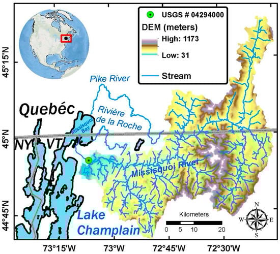
Figure 2. Focal study area of Missisquoi river watershed and Missisquoi bay situated in the transboundary north-eastern arm of the Lake Champlain basin in USA and Canada.

2.2. Estimation Procedures for Emulators

Three machine learning models—random forest [48], LightGBM [49] and XGBoost [50]—are trained on ~3.8 million observations for ~52 features derived from 332 scenarios simulated in the process-based CHANS [32,33]. Table A1 provides descriptive statistics for all variables used to train six specifications of these three types of ML models. The regression random forest (RRF), regression LightGBM (RLGBM) and regression XGBoost (RXGB) models predict the average surface mean of ChlA. Further, the classifier random forest (CRF), classifier LightGBT (CLGBM) and classifier XGBoost (CXGB) predict four trophic states of Missisquoi Bay derived from process-based CHANS. The python code for all six of these emulator models is made publicly available (see Data Availability Statement section).

In all six ML models, 80% of the ~3.8 million observations are randomly sampled for training the models while the remaining 20% are used to test the trained models. Hyperparameters for each of the six emulator models are described in the publicly available Python code. To avoid overfitting, hyperparameter tuning was not implemented. Further, in addition to adding 50 state variables from different components of CHANS, a random variable was also added in all six models. The random variable provides an entropy-based information theoretic metric to rank order the relative importance of 50 features predicting target variables in machine learning models [51,52,53,54,55]. Internal-to-the-lake biogeochemical processes predicting lake trophic states are captured by 6 RCA output variables (Table A1). RCA is part of the lake water quality AE2M model used in CHANS (Figure 1). External to the lake, the hydrological model (RHESSys) provides information on six variables representing the hydro-terrestrial processes of the watershed feeding into Missisquoi Bay (Table A1). Under the derived hydrology category, 9 variables representing river discharge and P and N fluxes into the Bay are derived from the CHANS simulation of three tributaries (Missisquoi, Rock and Pike rivers) feeding into the focal bay (Figure 2 and Table A1). Using CMIP5 downscaled data for Lake Champlain, four RCP scenarios were sampled from 9 GCMs (descriptive statistics in Table A1). Not all GCMs simulate all four RCPs. Figure 3 shows boxplots for the average surface mean of ChlA for four RCPs.

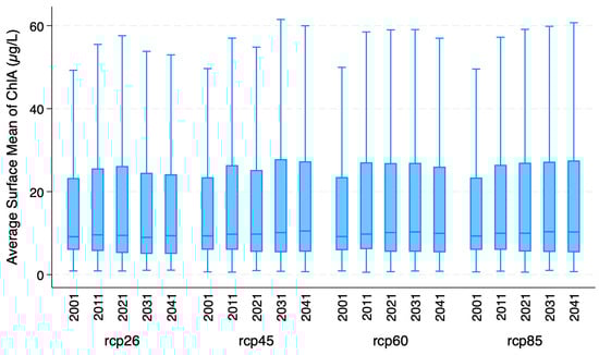
Figure 3. Boxplots of average surface mean of ChlA for four RCPs.

Further, eleven nutrient management scenarios, described in Table A1, were used to simulate human (policy maker) feedback to co-evolving lake water quality conditions. The current policy scenario, simulating EPA’s mandated 64.3% P reduction scenario is one of the 11 scenarios. The other 10 scenarios were developed in consultation with a stakeholder-derived Policy and Technical Committee, including 0%, 20%, 40%, 60%, 80% and 100% P reductions initiated in 2021. These eleven scenarios are discussed in detail in Zia et al. [33]. Four additional P management scenarios (S0 to S4), discussed in detail by Zia et al. [32], captured early vs. delayed action on addressing water quality concerns in the focal bay. Figure 4 shows boxplots of the average surface mean of ChlA for these combined 11 P management scenarios derived from three different studies. Both Figure 3 and Figure 4 show that GCC and nutrient management significantly impact the variability of ChlA at annual to decadal scales. Worst case GCC scenarios, i.e., RCP85 in Figure 3, increase the average annualized ChlA, while conversely, early action scenarios (S1 and S3 in Figure 4) reduce the average ChlA. Delayed or no action, i.e., the 0% P reduction scenario, produces the highest ChlA, which can be further aggravated if GCC-induced extreme events, i.e., floods, move large pulses of P from watersheds into the bay, as shown in S2 and S4 scenarios of Figure 4.

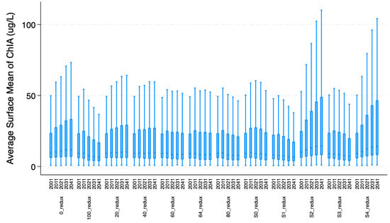
Figure 4. Boxplots of average surface mean of ChlA for 11 nutrient management scenarios. Decadal means and standard deviations for each P management scenario are presented.

3. Results

3.1. Machine-Learned Emulators

The RRF, RLGBM and RXGB emulator models are successfully able to reproduce histograms of the average surface mean of ChlA in the test data, as shown in Figure 5. The RXGB has the highest R² of 96% and the lowest RMSE (Table 1). The RLGBM and RRF also appear fairly robust with 95% and 93% R², respectively (Table 1).

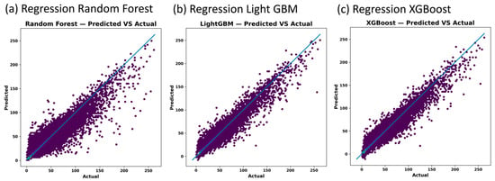
Figure 5. Emulator model predicted vs. actual (derived from CHANS model) average surface mean of ChlA in Missisquoi Bay from regression random forest (panel (a)), regression light GBM (panel (b)) and regression XGBoost (panel (c)).

Table 1. Regression model fitness scores.

Model	MAE	RMSE	MAPE	R2
Random Forest	2.12	4.91	13.59	0.93
LightGBM	2.27	4.06	16.73	0.95
XGBoost	1.72	3.49	12.45	0.96

The CLGBM attained the highest F1 score (96.15%), followed closely by CXGB (95.66%) and CRF (93.06%) (Table 2). A breakdown of the Precision, Recall and F1 scores for each of the four predicted trophic states are shown in Table 3 and the confusion matrices in Figure 6. The CLGBM’s ability to accurately predict oligotrophic and hyper-eutrophic states is 91.98% and 92.40% respectively, while it predicts mesotrophic and eutrophic states with a relatively higher accuracy at 97.96% and 95.16%, respectively.

Table 2. Classification model fitness scores.

Model	Precision	Recall	F1 Scores
Random Forest	93.12	93.12	93.06
XGBoost	95.65	95.66	95.66
LightGBM	96.15	96.16	96.15

Table 3. Classification prediction scores for each trophic state.

Predicted Class	Precision	Recall	F1-Score
Classifier Random Forest Model
Oligotrophic	0.9570	0.82	0.8859
Mesotrophic	0.9567	0.9681	0.9623
Eutrophic	0.9019	0.9286	0.9151
Hypereutrophic	0.9138	0.8037	0.8552
Classifier Light GBM
Oligotrophic	0.9437	0.8970	0.9198
Mesotrophic	0.9785	0.9806	0.9796
Eutrophic	0.9485	0.9547	0.9516
Hypereutrophic	0.9345	0.9138	0.9240
Classifier XGBoost
Oligotrophic	0.9546	0.8937	0.9231
Mesotrophic	0.9756	0.9781	0.9769
Eutrophic	0.9421	0.9479	0.9450
Hypereutrophic	0.9235	0.9043	0.9138

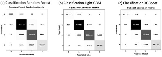
Figure 6. Accuracy rates for each of the four predicted trophic states derived from classifier random forest (panel (a)), classifier LightGBM (panel (b)) and classifier XGBoost (panel (c)) application on testing data. Label values on both x- and y-axis refer to 0 = oligotrophic; 1 = mesotrophic; 2 = eutrophic and 3 = hyper-eutrophic state.

3.2. Uncertainty Quantification and Teleconnections

Feature importances, shown in Table 4 and Table 5, are derived by SKLearn using the mean decrease in impurity (MDI). Table 4 presents feature importances for RRF, RLGBM and RXGB emulator models that predicted continuous ChlA. Table 5 shows feature importances derived from CRF, CLGBM and CXGB models that predicted four trophic states of Missisquoi Bay during the study period under alternate hydro-climatic and nutrient management scenarios. The rankings of all 50 features in each of these two tables across six emulator models can be interpreted by both evaluating the magnitude of the importance rate and assessing whether a feature provides more information than a maximum entropy random variable.

Table 4. Feature importances derived by SKLearn using mean decrease in impurity (MDI) for RRF, RLGBM and RXGB models predicting continuous ChlA.

	Random Forest Model		LightGBM Model		XGBoost
No.	Features	Importance	Features	Importance	Features	Importance
1	JPO4	0.287729	JPO4	0.26522	0_redux	0.10656
2	POPR	0.109358	snowpack	0.159382	JPO4	0.077549
3	JPON	0.10622	JPON	0.105759	S4_redux	0.065863
4	sat_def	0.090995	POPR	0.092713	snowpack	0.055426
5	snowpack	0.086359	sat_def	0.082248	gfdl-esm2m.1	0.044624
6	PO4T2R	0.085574	PO4T2R	0.068385	miroc-esm.1	0.040734
7	JPOP	0.059167	JPOP	0.06173	JPON	0.035666
8	baseflow	0.022333	evap	0.022808	sat_def	0.033486
9	%sat_area	0.018513	%sat_area	0.021349	POPR	0.032793
10	0_redux	0.017991	baseflow	0.021025	mri-cgcm3.1	0.031535
11	evap	0.016577	0_redux	0.013934	noresm1-m.1	0.030706
12	mri-cgcm3.1	0.007068	pike_TP	0.007113	canesm2.1	0.029454
13	noresm1-m.1	0.006373	mri-cgcm3.1	0.006814	S2_redux	0.028656
14	miroc-esm.1	0.006246	noresm1-m.1	0.006297	PO4T2R	0.027717
15	ccsm4.1	0.005241	streamflow	0.006265	JPOP	0.025247
16	gfdl-esm2m.1	0.005103	missisquoi_TP	0.005444	ccsm4.1	0.0238
17	pike_TP	0.004589	miroc-esm.1	0.005205	basin_TN_gps	0.022494
18	missisquoi_TP	0.004564	ccsm4.1	0.004781	pike_TN	0.022414
19	rock_TP	0.004527	trans	0.004062	20_redux	0.017224
20	streamflow	0.004387	rcp85	0.003764	rcp45	0.015557
21	RandomNum	0.004144	rock_TP	0.003586	rcp85	0.014869
22	rcp85	0.00411	S4_redux	0.003427	missisquoi_TP	0.013824
23	rcp60	0.00385	rcp45	0.003059	pike_TP	0.013381
24	trans	0.003554	rcp60	0.002743	rock_TP	0.012564
25	basin_TP_gps	0.003306	missisquoi_Q	0.002709	rcp60	0.01245
26	rcp45	0.003131	gfdl-esm2m.1	0.00232	60_redux	0.011888
27	S4_redux	0.002717	pike_TN	0.001869	100_redux	0.010429
28	canesm2.1	0.002629	rock_TN	0.001729	%sat_area	0.010406
29	S2_redux	0.002148	rock_Q	0.001712	missisquoi_Q	0.010406
30	pike_TN	0.001976	pike_Q	0.001681	S1_redux	0.009953
31	missisquoi_TN	0.00196	canesm2.1	0.001596	rcp26	0.009949
32	missisquoi_Q	0.001931	basin_TP_gps	0.001407	baseflow	0.009673
33	basin_TN_gps	0.001913	basin_TN_gps	0.001385	evap	0.008914
34	rock_TN	0.00189	S2_redux	0.001307	rock_TN	0.008367
35	pike_Q	0.001856	rcp26	0.001035	S0_redux	0.008351
36	rock_Q	0.001845	missisquoi_TN	0.001001	pike_Q	0.007178
37	20_redux	0.001678	S1_redux	0.000646	missisquoi_TN	0.007067
38	rcp26	0.001372	RandomNum	0.000614	40_redux	0.006701
39	S1_redux	0.001217	inmcm4.1	0.000366	80_redux	0.006283
40	40_redux	0.000733	20_redux	0.000277	streamflow	0.005903
41	S0_redux	0.000676	miroc-esm-chem.1	0.000221	trans	0.005435
42	S3_redux	0.000535	100_redux	0.000177	inmcm4.1	0.005432
43	60_redux	0.000406	40_redux	0.00016	S3_redux	0.00479
44	64_redux	0.00037	S3_redux	0.00016	basin_TP_gps	0.004218
45	inmcm4.1	0.000323	ipsl-cm5a-mr.1	0.000128	64_redux	0.003713
46	100_redux	0.000316	S0_redux	0.000113	miroc-esm-chem.1	0.003645
47	miroc-esm-chem.1	0.000194	60_redux	0.0001	ipsl-cm5a-mr.1	0.003206
48	ipsl-cm5a-mr.1	0.000161	64_redux	0.000094	rock_Q	0.002245
49	80_redux	0.000144	80_redux	0.000078	RandomNum	0.001254
50	PO4JRES	0	PO4JRES	0	PO4JRES	0

Table 5. Feature importances derived by SKLearn using mean decrease in impurity (MDI) for CRF, CLGBM and CXGB models predicting trophic states: oligotrophic; mesotrophic; eutrophic and hyper-eutrophic.

	Random Forest Model		LightGBM Model		XGBoost
No.	Features	Importance	Features	Importance	Features	Importance
1	JPO4	0.174135	sat_def	0.451271	0_redux	0.162563
2	snowpack	0.088807	PO4T2R	0.117711	snowpack	0.069072
3	JPON	0.087086	JPON	0.095367	JPO4	0.056315
4	POPR	0.072338	snowpack	0.054473	gfdl-esm2m.1	0.050352
5	JPOP	0.061633	RandomNum	0.052135	canesm2.1	0.040594
6	evap	0.059516	evap	0.047379	S4_redux	0.03954
7	sat_def	0.057572	JPO4	0.037579	S2_redux	0.037964
8	PO4T2R	0.043682	POPR	0.024385	JPON	0.031313
9	sat_area	0.042902	JPOP	0.020665	POPR	0.028901
10	baseflow	0.034019	baseflow	0.015573	60_redux	0.026905
11	pike_TP	0.018696	streamflow	0.015533	miroc-esm.1	0.021996
12	rock_TP	0.018348	%sat_area	0.01309	JPOP	0.018945
13	missisquoi_TP	0.018347	pike_TP	0.012963	rock_TP	0.018756
14	streamflow	0.016547	basin_TP_gps	0.006362	mri-cgcm3.1	0.018128
15	missisquoi_TN	0.016017	missisquoi_TP	0.005235	inmcm4.1	0.017671
16	rock_TN	0.015806	missisquoi_Q	0.004666	PO4T2R	0.017074
17	basin_TN_gps	0.015592	rock_TP	0.003397	sat_def	0.01596
18	pike_Q	0.015444	rock_TN	0.002987	ccsm4.1	0.015888
19	basin_TP_gps	0.01533	S4_redux	0.00249	noresm1-m.1	0.015487
20	rock_Q	0.015297	missisquoi_TN	0.002086	20_redux	0.015102
21	pike_TN	0.015199	trans	0.001732	rock_TN	0.014766
22	missisquoi_Q	0.015091	0_redux	0.001224	evap	0.014276
23	trans	0.013491	rcp85	0.00115	pike_Q	0.014007
24	RandomNum	0.01264	rock_Q	0.001026	S1_redux	0.01308
25	0_redux	0.005702	rcp45	0.000941	missisquoi_TN	0.012917
26	noresm1-m.1	0.005023	pike_TN	0.000845	100_redux	0.012649
27	mri-cgcm3.1	0.005021	gfdl-esm2m.1	0.000809	missisquoi_TP	0.012622
28	ccsm4.1	0.00446	pike_Q	0.000806	pike_TP	0.012354
29	miroc-esm.1	0.00426	ccsm4.1	0.000762	%sat_area	0.012291
30	rcp85	0.003901	mri-cgcm3.1	0.000692	baseflow	0.0113
31	gfdl-esm2m.1	0.003872	basin_TN_gps	0.000537	rcp26	0.01106
32	rcp45	0.003719	noresm1-m.1	0.000531	missisquoi_Q	0.010336
33	rcp60	0.003572	rcp60	0.000531	rcp60	0.010291
34	canesm2.1	0.003333	64_redux	0.000521	rcp45	0.009828
35	rcp26	0.002196	miroc-esm.1	0.000468	rcp85	0.009625
36	S1_redux	0.001335	canesm2.1	0.000441	trans	0.008985
37	inmcm4.1	0.001283	80_redux	0.000438	streamflow	0.00877
38	60_redux	0.001077	rcp26	0.000242	S0_redux	0.008641
39	S2_redux	0.001037	S2_redux	0.000167	pike_TN	0.008479
40	S0_redux	0.000932	inmcm4.1	0.000157	rock_Q	0.008107
41	S3_redux	0.000931	miroc-esm-chem.1	0.000128	S3_redux	0.007825
42	S4_redux	0.000833	60_redux	0.000094	miroc-esm-chem.1	0.00776
43	64_redux	0.000806	20_redux	0.000089	40_redux	0.007487
44	20_redux	0.000637	S1_redux	0.000083	basin_TP_gps	0.006696
45	40_redux	0.000564	ipsl-cm5a-mr.1	0.000082	64_redux	0.006549
46	miroc-esm-chem.1	0.000529	S3_redux	0.000055	basin_TN_gps	0.006182
47	80_redux	0.000487	40_redux	0.000052	ipsl-cm5a-mr.1	0.005993
48	100_redux	0.000478	S0_redux	0.000028	80_redux	0.005598
49	ipsl-cm5a-mr.1	0.000477	100_redux	0.000023	RandomNum	0.003002
50	PO4JRES	0	PO4JRES	0	PO4JRES	0

In all six machine-learned emulator models, consistent with computational aquatic ecology, this study discovers that the following internal-to-the-lake features emerge as the leading drivers of water quality regime shifts: Phosphate flux to water column (JPO4) ranked as the #1 feature in RRF (28.77 importance %), #1 in RLGBM (26.52 importance %); #2 in RXGB (7.75%), #1 in CRF (17.41%), #3 in CXGB (5.63%) and #7 in CLGBM (3.75%). Except for CLGBM, JPO4 scores a higher importance % than a random number feature in five other machine learning models. Other highly ranked internal-to-the-lake importance features in emulator models include particulate organic nitrogen water–sediment flux (JPON); total particulate organic phosphorus (POPR); and PO4 resuspension flux (PO4T2R) (Table 4 and Table 5).

Novel findings derived from the analysis of feature importances shown in Table 4 and Table 5 emerge from the consideration of important features that are external-to-the-lake model, which are captured in the integrated CHANS model through hydro-climatic and nutrient management features. It is discovered that Snow Water Equivalent (SWE) over the entire watershed (snowpack) and Saturation deficit (volume) over entire watershed (sat_def) emerge as top ranked features in all six emulator models (Table 4 and Table 5). Snowpack is ranked #5 in RRF (8.63%), #2 in RLGBM (15.93%), #4 in RXGB (5.54%), #2 in CRF (8.88%), #4 in CLGBM (5.54%) and #2 in RXGB (6.9%). Furthermore, evaporation over entire watershed (evap), % saturated area over entire watershed (% sat area) and baseflow measured at USGS gauges (baseflow) emerged as three additional, external to the lake, features among the top ranked features in all six models. Additional features in both emulators represented slightly different configurations of nutrient management and global climate change scenarios and their consequent impacts on the predicted nutrient fluxes (i.e., TP) and streamflow in the process-based integrated CHANS model.

In the case of applications in the Missisquoi Bay of the Lake Champlain, it is discovered from the analysis of feature importances (Table 4 and Table 5) that predictor variables representing snow, saturation, evaporation, transpiration, baseflow, streamflow and TP flux teleconnect hydro-climatic processes occurring in terrestrial watersheds with the biogeochemical processes occurring in the freshwater lakes.

For explaining the marginal effects of higher importance-ranked internal-to-the-lake biogeochemical processes and external-to-the-lake teleconnections, we highlight 12 features and show their partial dependence plots (PDPs) from RRF (Figure 7), RLGBM (Figure 8), RXGB (Figure 9) and CLGBM, with four trophic regimes—oligotrophic (Figure 10), mesotrophic (Figure 11), eutrophic (Figure 12) and hyper-eutrophic (Figure 13). PDPs for four trophic regimes estimated for CRF are shown in Figure A1, Figure A2, Figure A3 and Figure A4 and CXGB in Figure A5, Figure A6, Figure A7 and Figure A8. Generally, if a PDP is flat, the feature has little influence, but if PDP varies significantly, a feature strongly affects predictions. Nonlinear shapes (e.g., U-shaped, thresholds) indicate complex interactions in Figure 7, Figure 8, Figure 9, Figure 10, Figure 11, Figure 12 and Figure 13 and Figure A1, Figure A2, Figure A3, Figure A4, Figure A5, Figure A6, Figure A7 and Figure A8.

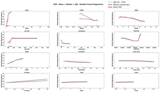
Figure 7. Partial Dependence Plots derived from RRF for important features. The plots display the mean, median and interquartile range (IQR) of predicted values across bootstrap replicates. Rug marks along the x-axis indicate the observed feature values in the dataset, providing context on the distribution of input data.

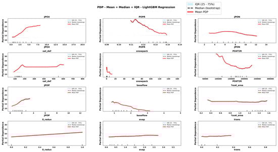
Figure 8. Partial Dependence Plots derived from RLGBM for important features. The plots display the mean, median and interquartile range (IQR) of predicted values across bootstrap replicates. Rug marks along the x-axis indicate the observed feature values in the dataset, providing context on the distribution of input data.

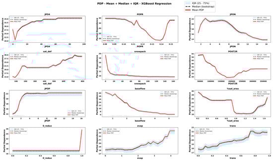
Figure 9. Partial Dependence Plots derived from RXGB for important features. The plots display the mean, median and interquartile range (IQR) of predicted values across bootstrap replicates. Rug marks along the x-axis indicate the observed feature values in the dataset, providing context on the distribution of input data.

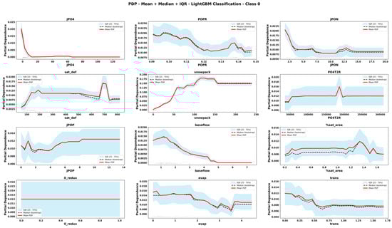
Figure 10. Partial Dependence Plots derived from CLGBM for important features for Oligotrophic state. The plots display the mean, median and interquartile range (IQR) of predicted values across bootstrap replicates. Rug marks along the x-axis indicate the observed feature values in the dataset, providing context on the distribution of input data.

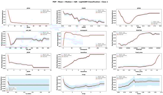
Figure 11. Partial Dependence Plots derived from CLGBM for important features for mesotrophic state. The plots display the mean, median and interquartile range (IQR) of predicted values across bootstrap replicates. Rug marks along the x-axis indicate the observed feature values in the dataset, providing context on the distribution of input data.

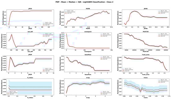
Figure 12. Partial Dependence Plots derived from CLGBM for important features for eutrophic state. The plots display the mean, median and interquartile range (IQR) of predicted values across bootstrap replicates. Rug marks along the x-axis indicate the observed feature values in the dataset, providing context on the distribution of input data.

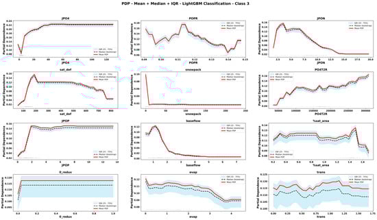
Figure 13. Partial Dependence Plots derived from CLGBM for important features for hypereutrophic state. The plots display the mean, median and interquartile range (IQR) of predicted values across bootstrap replicates. Rug marks along the x-axis indicate the observed feature values in the dataset, providing context on the distribution of input data.

To improve the interpretability and robustness of the Partial Dependence Plots (PDPs), a bootstrap-based approach was implemented. For each PDP, predictions were generated using a bootstrap sample of 500 observations drawn from the training dataset, allowing variability in the marginal effects of the selected features to be captured. Three summary statistics were presented for each feature: the mean, median and interquartile range (IQR) of predicted values across the bootstrap replicates. These measures provide insight into both central tendency and dispersion, rather than relying solely on the conditional mean. Additionally, rug marks (small tick marks along the x-axis) were included to indicate the observed values of the feature in the dataset, offering context on the distribution of feature values. This combination of bootstrap sampling, variability measures and data distribution indicators enhances the interpretative value of the PDPs and addresses potential concerns about over-reliance on average effects.

The comparison of PDPs derived from six emulator models provides novel information about the teleconnected processes and thresholds among coupled co-varying natural and social system dynamics. Focusing on internal lake processes, for example, RLGBM PDPs (Figure 8) show that JPO4 has an exponential effect on increasing ChlA; however, CLGBM PDPs show four different shapes of JPO4 effects under each of the four alternate trophic states of the lake. In oligotrophic conditions (Figure 10), phosphate flux increases in the water column has a decreasing impact on ChlA. A similar threshold decreasing impact, stabilizing after the threshold, is also predicted for JPO4 by the CLGBM emulator model during the mesotrophic state (Figure 11). In contrast, during the eutrophic (Figure 12) and hyper-eutrophic states (Figure 13), JPO4 has a rapid and exponential impact on triggering ChlA. Partial dependence plots for JPO4 derived from other classifier models (i.e., CRF and CXGB shown in Figure A1, Figure A2, Figure A3, Figure A4, Figure A5, Figure A6, Figure A7 and Figure A8) also predict similar marginal effects of JPO4. As opposed to JPO4, JPON increments lead to a proportional decrease in continuous ChlA. Since Misssiquoi Bay is P limited [56], JPON’s average decreasing impact is consistent with theoretical expectations (Figure 7, Figure 8 and Figure 9). In mesotrophic states (Figure 11), JPON has a slightly increasing effect on ChlA; and in eutrophic and hyper-eutrophic conditions, JPON suppresses ChlA (Figure 10 and Figure 11).

CHANS emulator models advance understanding of telecoupled and teleconnected processes in social ecological systems. Analysis of PDPs for features external to the lake influencing ChlA provides a rigorous mechanism to discover the effect sizes of relatively important teleconnections on both continuous ChlA and alternate trophic states. The Snow Water Equivalent (SWE) over entire watershed is expected to decrease across different long term GCC scenarios; and increasing SWE (Figure 7, Figure 8 and Figure 9) slightly lowers the likelihood of continuous ChlA. This effect is, however, more pronounced with strong threshold effects in eutrophic and hyper-eutrophic states (Figure 10 and Figure 11). Another set of relatively important teleconnection concerns the saturation deficit and the fraction of the saturated area over the entire watershed, both of which are important modulator variables signifying dry and wet hydroclimatic regimes in watersheds. A higher saturation deficit, signifying drought-like conditions over the watersheds, has a strong threshold based effect on increasing the likelihood of continuous ChlA (Figure 7, Figure 8 and Figure 9). Similarly, as the fraction of saturated area goes above a threshold, continuous ChlA has a slight decreasing effect. In contrast, increases in evaporation and transpiration has slightly increasing effect on continuous ChlA (Figure 7, Figure 8 and Figure 9). The impacts of hydroclimatic variables are generally consistent among six emulator model derived PDPs, with a few exceptions.

4. Discussion

The emulator models support both computational efficiency and enable “explainable AI” [57,58], exemplified in this study through interpretation of MDI generated feature importance ranks (Table 4 and Table 5) and PDPs (Figure 7, Figure 8, Figure 9, Figure 10, Figure 11, Figure 12 and Figure 13 and Figure A1, Figure A2, Figure A3, Figure A4, Figure A5, Figure A6, Figure A7 and Figure A8). Using information theoretic metrics of ascertaining feature importance, machine-learned emulator models provide parametric free approaches to quantify uncertainty in complex models. The quantification of uncertainty across coupled models also enables discovery of teleconnections and telecouplings. In this study, it is discovered that both internal-to-the-lake and external watershed-driven hydro-climatic and social processes are telecoupled and a better understanding of these teleconnections can provide critical insights for nutrient management processes in the face of global climate change induced shifts in eco-hydrological regimes and extreme events through shifts in Snow Water Equivalent, saturation deficit over watershed, fraction of the saturated watershed, and vegetation cover induced shifts in evaporation and transpiration. This finding is consistent with the growing body of empirical literature on “short water cycle” in eco-hydrological and socio-hydrological studies [59,60,61,62]. While process-based CHANS models can simulate these processes and couplings with more process-complexity and granularity, the machine-learned emulator models can learn from process-based CHANS models and enable discovery of teleconnections.

There are also significant limitations of emulator models of CHANS that need to be considered for explaining, understanding and managing the coupled natural and human systems processes. One of the major limitations concerns coarser granularity of emulator model predictors vis-à-vis predictors of process-based CHANS models. While computational efficiency is gained at the expense of spatial and temporal precision, the place-specific social ecological processes might be overlooked by emulator models. Another important limitation concerns the sampling of predictor features and target variables. While unsupervised and semi-supervised machine learning approaches can be tested in future research to design emulator models, the supervised machine-learned emulator models presented in this study could be sensitive to the choice of features tested for ascertaining feature importance. Further, while computationally efficient compared with process-based models, the emulator models presented in this study still required significant amount of computational resources that limited our capacity to run large scale uncertainty tests by systematically adding or deleting different sets of feature variables. Finally, an important area of future research concerns the ability of emulator models to accurately predict out-of-training sample, external validation, and ground-truthing earth observation data.

The emulator is trained/tested on simulated CHANS outputs, not real-world observational datasets. Thus, its predictive ability beyond model-generated data is uncertain. Incorporating field data (chlorophyll-a, nutrient fluxes, snowpack records) to test emulator predictions must be a high priority for future research. There are, however, significant barriers to undertaking this validation with the field data. The most insurmountable barrier is the sheer absence of field data. For example, the process-based 4D lake simulation model A2EM predicts ChlA and other lake water quality variables at ~180 m × 180 m pixel size for ~five vertical layers to account for subsurface dynamics. The emulator model is trained to predict the geographical average of the surface layer of ChlA. There is no consistently measured gridded data set available to compare against. The CHANS model was calibrated against long term monitoring data, which is effectively one point in the Bay; and a high frequency sensor data on a nearby point. Field data on many other CHANS variables, e.g., subsurface dissolved oxygen, is also not consistently and reliably collected by management agencies. While remote sensing science is rapidly advancing to leverage satellite data sets, e.g., surface layer ChlA predicted by Sentinel 2 and 3 missions [47], as validation data sets, there are many difficult technical and logistical challenges to enable this comparison at this stage. Most importantly, Sentinel 2 and 3 predictions are made in units of spectral densities for the surface layer, inconsistently observed once or twice a week due to cloud cover issues, while the CHANS simulations make numerical predictions for the entire 4D grid. Similar challenges with respect to paucity of data exist for the measurement of watershed-level variables such as SWE, evaporation and saturation deficit. Emulator model based forecasting with field data validation is an interesting area of investigation for future research.

5. Conclusions

Confirming our main hypothesis, it is demonstrated in this study that machine-learned emulator models provide data-driven methods to discover teleconnections and quantify uncertainty in complex multi-sector models of coupled natural and human systems. All six emulator models generate similar list of uncertainty-inducing predictors of water quality in the coupled system. However, differences are also observed in relative rankings and quantitative estimates of uncertainties induced by coupled state variables and their respective importance in predicting continuous ChlA, a proxy metric of water quality measurement in freshwater lakes, as well as alternate eutrophic states of freshwater lakes. Lack of earth observation data limits the ability of emulator models to be tested for their forecast skill.

Despite limitations in availability of earth observation data, our proposed approach to measure and interpret machine-learned emulator models of process-based CHANS models can be scaled up in different watersheds and lakes to discover teleconnections and quantify uncertainty of different internal-to-the-lake and external-to-the-lake features driving integrated water quantity and water quality processes. Further, this machine-learned emulator modeling approach can also be tested and scaled to investigate drivers of change in CHANS models focused on predicting GCC-induced extreme events, e.g., floods and droughts, and their co-evolving impacts on nutrient fluxes, LULCC, watershed management and freshwater lake water quality. Major pathways to implement the proposed ensemble emulator models in these domains include access to the data and model code for process-based models simulating these processes, sampling appropriate target and predictor features, testing model accuracy, discovering teleconnections, and quantifying uncertainty. Testing emulator predictions against earth observation datasets will further enhance the reliability and robustness of the ensemble emulator models. Finally, with increasing availability of earth system data through satellites, drones and in situ sensors, more advanced and dynamic emulator models may be trained and tested in future applications.

References

- Miller, T.; Durlik, I.; Kostecka, E.; Kozlovska, P.; Łobodzińska, A.; Sokołowska, S.; Nowy, A. Integrating artificial intelligence agents with the internet of things for enhanced environmental monitoring: Applications in water quality and climate data. Electronics 2025, 14, 696. [Google Scholar] [CrossRef]
- Sharma, S.; Sharma, K.; Grover, S. Real-time data analysis with smart sensors. In Application of Artificial Intelligence in Wastewater Treatment; Springer: Berlin/Heidelberg, Germany, 2024; pp. 127–153. [Google Scholar]
- Gani, A.; Hussain, A.; Pathak, S.; Omar, P.J. Analysing heavy metal contamination in groundwater in the vicinity of Mumbai’s landfill sites: An in-depth study. Top. Catal. 2024, 67, 1009–1023. [Google Scholar] [CrossRef]
- Pan, D.; Deng, Y.; Yang, S.X.; Gharabaghi, B. Recent Advances in Remote Sensing and Artificial Intelligence for River Water Quality Forecasting: A Review. Environments 2025, 12, 158. [Google Scholar] [CrossRef]
- Reichstein, M.; Camps-Valls, G.; Stevens, B.; J, M.; Denzler, J.; Carvalhais, N.; Prabhat, F. Deep learning and process understanding for data-driven Earth system science. Nature 2019, 566, 195–204. [Google Scholar] [CrossRef]
- Zia, A. Towards the Deployment of Food, Energy and Water Security Early Warning Systems as Convergent Technologies for Building Climate Resilience. In The Water, Energy, and Food Security Nexus in Asia and the Pacific: Central and South Asia; Springer International Publishing: Cham, Switzerland, 2024; pp. 99–118. [Google Scholar]
- Droegemeier, K.; Kontos, C.; Kratsios, M.; Córdova, F.; Walker, S.; Parker, L.; Romine, C.; Kurose, J.; Binkley, S. The National Artificial Intelligence Research and Development Strategic Plan: 2019 Update; National Science & Technology Council: Washington, DC, USA, 2019. [Google Scholar]
- Carter, J.; Feddema, J.; Kothe, D.; Neely, R.; Pruet, J.; Stevens, R.; Balaprakash, P.; Beckman, P.; Foster, I.; Iskra, K. Advanced Research Directions on AI for Science, Energy, and Security: Report on Summer 2022 Workshops; U.S. Department of Energy: Oak Ridge, TN, USA, 2023. [Google Scholar]
- Liu, J.; Hull, V.; Batistella, M.; DeFries, R.; Dietz, T.; Fu, F. Telecoupling: A new frontier for global sustainability. Ecol. Soc. 2013, 18, 26. [Google Scholar]
- Friis, C.; Nielsen, J.Ø. From teleconnection to telecoupling: Taking stock of an emerging framework in land system science. J. Land Use Sci. 2015, 10, 214–230. [Google Scholar] [CrossRef]
- Hüllermeier, E.; Waegeman, W. Aleatoric and epistemic uncertainty in machine learning: An introduction to concepts and methods. Mach. Learn. 2021, 110, 457–506. [Google Scholar] [CrossRef]
- Schmelzer, M.; Dwight, R.P.; Cinnella, P. Discovery of algebraic Reynolds-stress models using sparse symbolic regression. Flow Turbul. Combust. 2020, 104, 579–603. [Google Scholar] [CrossRef]
- Runge, J.; Bathiany, S.; Bollt, E.; Camps-Valls, G.; Coumou, D.; Deyle, E.; Glymour, C.; Kretschmer, M.; Mahecha, M.D.; Muñoz-Marí, J. Inferring causation from time series in Earth system sciences. Nat. Commun. 2019, 10, 2553. [Google Scholar] [CrossRef] [PubMed]
- Robinson, D.T.; Di Vittorio, A.; Alexander, P.; Arneth, A.; Barton, C.M.; Brown, D.G.; Kettner, A.; Lemmen, C.; O’neill, B.C.; Janssen, M. Modelling feedbacks between human and natural processes in the land system. Earth Syst. Dyn. 2018, 9, 895–914. [Google Scholar] [CrossRef]
- Calvin, K.; Bond-Lamberty, B. Integrated human-earth system modeling—State of the science and future directions. Environ. Res. Lett. 2018, 13, 063006. [Google Scholar] [CrossRef]
- Saltelli, A.; Ratto, M.; Andres, T.; Campolongo, F.; Cariboni, J.; Gatelli, D.; Saisana, M.; Tarantola, S. Global Sensitivity Analysis: The Primer; John Wiley & Sons: Hoboken, NJ, USA, 2008. [Google Scholar]
- Paxton, P.; Curran, P.J.; Bollen, K.A.; Kirby, J.; Chen, F. Monte Carlo experiments: Design and implementation. Struct. Equ. Model. 2001, 8, 287–312. [Google Scholar] [CrossRef]
- Willems, P. Model uncertainty analysis by variance decomposition. Phys. Chem. Earth Parts A/B/C 2012, 42, 21–30. [Google Scholar] [CrossRef]
- Wang, X.; Wang, L. Uncertainty quantification and propagation analysis of structures based on measurement data. Math. Comput. Model. 2011, 54, 2725–2735. [Google Scholar] [CrossRef]
- Vrugt, J.A.; Gupta, H.V.; Bouten, W.; Sorooshian, S. A Shuffled Complex Evolution Metropolis algorithm for optimization and uncertainty assessment of hydrologic model parameters. Water Resour. Res. 2003, 39, 1201. [Google Scholar] [CrossRef]
- Tolson, B.A.; Shoemaker, C.A. Dynamically dimensioned search algorithm for computationally efficient watershed model calibration. Water Resour. Res. 2007, 43, W01413. [Google Scholar] [CrossRef]
- Le, X.-H.; Huynh, T.T.; Song, M.; Lee, G. Quantifying predictive uncertainty and feature selection in river bed load estimation: A multi-model machine learning approach with particle swarm optimization. Water 2024, 16, 1945. [Google Scholar] [CrossRef]
- Wu, B.; Zheng, Y.; Tian, Y.; Wu, X.; Yao, Y.; Han, F.; Liu, J.; Zheng, C. Systematic assessment of the uncertainty in integrated surface water-groundwater modeling based on the probabilistic collocation method. Water Resour. Res. 2014, 50, 5848–5865. [Google Scholar] [CrossRef]
- Guzman, J.A.; Shirmohammadi, A.; Sadeghi, A.M.; Wang, X.; Chu, M.L.; Jha, M.K.; Parajuli, P.B.; Harmel, R.D.; Khare, Y.P.; Hernandez, J.E. Uncertainty considerations in calibration and validation of hydrologic and water quality models. Trans. ASABE 2015, 58, 1745–1762. [Google Scholar] [CrossRef]
- Yapo, P.O.; Gupta, H.V.; Sorooshian, S. Multi-objective global optimization for hydrologic models. J. Hydrol. 1998, 204, 83–97. [Google Scholar] [CrossRef]
- Vrugt, J.A.; Ter Braak, C.J. DREAM (D): An adaptive Markov Chain Monte Carlo simulation algorithm to solve discrete, noncontinuous, and combinatorial posterior parameter estimation problems. Hydrol. Earth Syst. Sci. 2011, 15, 3701–3713. [Google Scholar] [CrossRef]
- Thyer, M.; Renard, B.; Kavetski, D.; Kuczera, G.; Franks, S.W.; Srikanthan, S. Critical evaluation of parameter consistency and predictive uncertainty in hydrological modeling: A case study using Bayesian total error analysis. Water Resour. Res. 2009, 45, W00B14. [Google Scholar] [CrossRef]
- Beven, K.; Binley, A. The future of distributed models: Model calibration and uncertainty prediction. Hydrol. Process. 1992, 6, 279–298. [Google Scholar] [CrossRef]
- Gong, W.; Duan, Q.; Li, J.; Wang, C.; Di, Z.; Ye, A.; Miao, C.; Dai, Y. Multiobjective adaptive surrogate modeling-based optimization for parameter estimation of large, complex geophysical models. Water Resour. Res. 2016, 52, 1984–2008. [Google Scholar] [CrossRef]
- Farahani, M.A.; Wood, A.W.; Tang, G.; Mizukami, N. Calibrating a large-domain land/hydrology process model in the age of AI: The SUMMA CAMELS emulator experiments. Hydrol. Earth Syst. Sci. 2025, 29, 4515–4537. [Google Scholar] [CrossRef]
- Bennett, A.; Tran, H.; De la Fuente, L.; Triplett, A.; Ma, Y.; Melchior, P.; Maxwell, R.M.; Condon, L.E. Spatio-temporal machine learning for regional to continental scale terrestrial hydrology. J. Adv. Model. Earth Syst. 2024, 16, e2023MS004095. [Google Scholar] [CrossRef]
- Zia, A.; Oikonomou, P.D.; Clemins, P.J.; Schroth, A.W. H11N-0864 Co-producing hydroclimatic forecasts and evaluating their impact on nutrient budgeting and abatement costs for securing clean water in transboundary Missisquoi bay of Lake Champlain, 2000–2050. In Proceedings of the AGU Fall Meeting Abstracts, Washington, DC, USA, 9–13 December 2024; Available online: https://agu.confex.com/agu/agu24/meetingapp.cgi/Paper/1573373 (accessed on 24 December 2025).
- Zia, A.; Schroth, A.W.; Hecht, J.S.; Isles, P.; Clemins, P.J.; Turnbull, S.; Bitterman, P.; Tsai, Y.; Mohammed, I.N.; Bucini, G. Climate change-legacy phosphorus synergy hinders lake response to aggressive water policy targets. Earth’s Future 2022, 10, e2021EF002234. [Google Scholar] [CrossRef]
- Wurtsbaugh, W.A.; Paerl, H.W.; Dodds, W.K. Nutrients, eutrophication and harmful algal blooms along the freshwater to marine continuum. Wiley Interdiscip. Rev. Water 2019, 6, e1373. [Google Scholar] [CrossRef]
- Feng, L.; Wang, Y.; Hou, X.; Qin, B.; Kutser, T.; Qu, F.; Chen, N.; Paerl, H.W.; Zheng, C. Harmful algal blooms in inland waters. Nat. Rev. Earth Environ. 2024, 5, 631–644. [Google Scholar] [CrossRef]
- Iiames, J.; Salls, W.; Mehaffey, M.; Nash, M.; Christensen, J.; Schaeffer, B. Modeling anthropogenic and environmental influences on freshwater harmful algal bloom development detected by MERIS over the central United States. Water Resour. Res. 2021, 57, e2020WR028946. [Google Scholar] [CrossRef]
- Lan, J.; Liu, P.; Hu, X.; Zhu, S. Harmful algal blooms in eutrophic marine environments: Causes, monitoring, and treatment. Water 2024, 16, 2525. [Google Scholar] [CrossRef]
- Igwaran, A.; Kayode, A.J.; Moloantoa, K.M.; Khetsha, Z.P.; Unuofin, J.O. Cyanobacteria harmful algae blooms: Causes, impacts, and risk management. Water Air Soil Pollut. 2024, 235, 71. [Google Scholar] [CrossRef]
- Woolway, R.I.; Zhang, Y.; Jennings, E.; Zohary, T.; Jane, S.F.; Jansen, J.; Weyhenmeyer, G.A.; Long, D.; Fleischmann, A.; Feng, L. Extreme and compound events in lakes. Nat. Rev. Earth Environ. 2025, 6, 593–611. [Google Scholar] [CrossRef]
- Zhao, G.; Li, K.; Tian, S.; Liang, R.; Wang, Y. Applying a coupled model framework to assess global climate change impacts on the river-type harmful algal blooms in the middle and lower reaches of the Hanjiang River, China. Ecol. Indic. 2024, 169, 112834. [Google Scholar] [CrossRef]
- Elhabashy, A.; Li, J.; Sokolova, E. Water quality modeling of a eutrophic drinking water source: Impact of future climate on Cyanobacterial blooms. Ecol. Model. 2023, 477, 110275. [Google Scholar] [CrossRef]
- Golub, M.; Thiery, W.; Marcé, R.; Pierson, D.; Vanderkelen, I.; Mercado, D.; Woolway, R.I.; Grant, L.; Jennings, E.; Schewe, J. A framework for ensemble modelling of climate change impacts on lakes worldwide: The ISIMIP Lake Sector. Geosci. Model Dev. Discuss. 2022, 15, 4597–4623. [Google Scholar] [CrossRef]
- Chapra, S.C.; Boehlert, B.; Fant, C.; Bierman, V.J., Jr.; Henderson, J.; Mills, D.; Mas, D.M.; Rennels, L.; Jantarasami, L.; Martinich, J. Climate change impacts on harmful algal blooms in US freshwaters: A screening-level assessment. Environ. Sci. Technol. 2017, 51, 8933–8943. [Google Scholar] [CrossRef] [PubMed]
- Lin, Q.; Zhang, K.; Giguet-Covex, C.; Arnaud, F.; McGowan, S.; Gielly, L.; Capo, E.; Huang, S.; Ficetola, G.F.; Shen, J. Transient social–ecological dynamics reveal signals of decoupling in a highly disturbed Anthropocene landscape. Proc. Natl. Acad. Sci. USA 2024, 121, e2321303121. [Google Scholar] [CrossRef]
- Celikkol, S.; Fortin, N.; Tromas, N.; Andriananjamanantsoa, H.; Greer, C.W. Bioavailable nutrients (N and P) and precipitation patterns drive cyanobacterial blooms in Missisquoi Bay, Lake Champlain. Microorganisms 2021, 9, 2097. [Google Scholar] [CrossRef] [PubMed]
- McCarthy, M.J.; Gardner, W.S.; Lehmann, M.F.; Bird, D.F. Implications of water column ammonium uptake and regeneration for the nitrogen budget in temperate, eutrophic Missisquoi Bay, Lake Champlain (Canada/USA). Hydrobiologia 2013, 718, 173–188. [Google Scholar] [CrossRef]
- Wynne, T.T. Remote sensing of cyanobacterial blooms in Lake Champlain with a focus on Missisquoi Bay. J. Great Lakes Res. 2024, 50, 102293. [Google Scholar] [CrossRef]
- Breiman, L. Random Forests. Mach. Learn. 2001, 45, 5–32. [Google Scholar] [CrossRef]
- Ke, G.; Meng, Q.; Finley, T.; Wang, T.; Chen, W.; Ma, W.; Ye, Q.; Liu, T.Y. LightGBM: A Highly Efficient Gradient Boosting Decision Tree. In Proceedings of the Advances in Neural Information Processing Systems, Long Beach, CA, USA, 4–9 December 2017; Volume 30, pp. 3146–3154. [Google Scholar]
- Chen, T.; Guestrin, C. XGBoost: A Scalable Tree Boosting System. In Proceedings of the Proceedings of the 22nd ACM SIGKDD International Conference on Knowledge Discovery and Data Mining, San Francisco, CA, USA, 13–17 August 2016; pp. 785–794. [Google Scholar]
- Battiti, R. Using Mutual Information for Selecting Features in Supervised Neural Net Learning. IEEE Trans. Neural Netw. 1994, 5, 537–550. [Google Scholar] [CrossRef] [PubMed]
- Kohavi, R.; John, G.H. Wrappers for Feature Subset Selection. In Proceedings of the International Journal of Artificial Intelligence, Atlanta, Georgia, 10–13 June 1997; pp. 273–324. [Google Scholar]
- Peng, H.; Long, F.; Ding, C. Feature Selection Based on Mutual Information: Criteria of Max-Dependency, Max-Relevance, and Min-Redundancy. IEEE Trans. Pattern Anal. Mach. Intell. 2005, 27, 1226–1238. [Google Scholar] [CrossRef] [PubMed]
- Quinlan, R. Induction of Decision Trees. Mach. Learn. 1986, 1, 81–106. [Google Scholar] [CrossRef]
- Shannon, C.E. A Mathematical Theory of Communication. Bell Syst. Tech. J. 1948, 27, 379–423. [Google Scholar] [CrossRef]
- Kincaid, D.W.; Adair, E.C.; Joung, D.; Stockwell, J.D.; Schroth, A.W. Ice cover and thaw events influence nitrogen partitioning and concentration in two shallow eutrophic lakes. Biogeochemistry 2022, 157, 15–29. [Google Scholar] [CrossRef]
- Salih, A.M.; Galazzo, I.B.; Raisi-Estabragh, Z.; Petersen, S.E.; Menegaz, G.; Radeva, P. Characterizing the contribution of dependent features in XAI methods. IEEE J. Biomed. Health Inform. 2024, 28, 6466–6473. [Google Scholar] [CrossRef]
- Casalicchio, G.; Molnar, C.; Bischl, B. Visualizing the feature importance for black box models. In Proceedings of the Joint European Conference on Machine Learning and Knowledge Discovery in Databases, Dublin, Ireland, 10–14 September 2018; Springer: Berlin/Heidelberg, Germany, 2018; pp. 655–670. [Google Scholar]
- Cao, Z.; Wang, S.; Luo, P.; Xie, D.; Zhu, W. Watershed Ecohydrological Processes in a Changing Environment. Water 2022, 14, 1234. [Google Scholar] [CrossRef]
- Gu, J.; Sun, S.; Wang, Y.B.; Li, X. Sociohydrology: An Effective Way to Reveal Coupled Evolution. Water Resour. Manag. 2021, 35, 123–139. [Google Scholar] [CrossRef]
- Li, B.; Sivapalan, M. Long-Term Coevolution of an Urban Human–Water System. Water Resour. Res. 2020, 56, e2019WR026123. [Google Scholar] [CrossRef]
- Marlow, D. Small Water Cycles: What They Are, Their Importance, Their Restoration; Water Research Australia: Adelaide, Australia, 2019. [Google Scholar]
Disclaimer/Publisher’s Note: The statements, opinions and data contained in all publications are solely those of the individual author(s) and contributor(s) and not of MDPI and/or the editor(s). MDPI and/or the editor(s) disclaim responsibility for any injury to people or property resulting from any ideas, methods, instructions or products referred to in the content. |
© 2025 by the authors. Licensee MDPI, Basel, Switzerland. This article is an open access article distributed under the terms and conditions of the Creative Commons Attribution (CC BY) license.