An Attention-Based Hybrid CNN–Bidirectional LSTM Model for Classifying Chlorophyll-a Concentration in Coastal Waters

Abstract

Accurate monitoring of chlorophyll-a (Chl-a) is essential for managing coastal aquaculture, as Chl-a indicates phytoplankton biomass and water quality. This study developed a hybrid deep learning model integrating convolutional neural networks (CNN), bidirectional long short-term memory (BiLSTM), and an attention mechanism (Attention) to classify Chl-a using hourly, water quality datasets collected from the GOT001 station in Si Racha Bay, Eastern Gulf of Thailand (2020–2024). A random forest (RF) identified sea surface temperature (SEATEMP), dew point temperature (DEWPOINT), and turbidity (TURB) as the most influential variables, accounting for over 90% of the accuracy. Chl-a concentrations were categorized into ecological groups (low, medium, and high) using quantile-based binning and K-means clustering to support operational classification. Model performance comparison showed that the CNN–BiLSTM model achieved the highest classification accuracy (81.3%), outperforming the CNN–LSTM model (59.7%). However, the addition of the Attention did not enhance predictive performance, likely due to the limited number of key predictive variables and their already high explanatory power. This study highlights the potential of CNN–BiLSTM as a near-real-time classification tool for Chl-a levels in highly variable coastal ecosystems, supporting aquaculture management, early warning of algal blooms or red tides, and water quality risk assessment in the Gulf of Thailand and comparable coastal regions.

1. Introduction

Aquaculture is an important source of protein that helps meet the increasing global demand for animal protein [1]. Many countries have promoted freshwater, brackish water, and marine aquaculture, particularly sea farming, which requires reliable management technologies and monitoring systems, including ground-truth data, to support sustainable management and production [2,3]. In Thailand, the coastal area of Si Racha, Chonburi Province, is regarded as a suitable and important aquaculture zone due to its nutrient inputs from the Chao Phraya and Bang Pakong Rivers, relatively stable temperature and salinity (SAL) throughout the year, and proximity to major consumer markets. However, during the southwest monsoon season, water quality can deteriorate, especially in terms of chlorophyll-a (Chl-a) concentration, which serves as an indicator of phytoplankton biomass and trophic status.

Chl-a concentrations are closely associated with the rapid growth of plankton, particularly cyanobacteria, which can trigger algal blooms or red tides that degrade water quality and affect coastal ecosystem stability [4,5,6,7]. Consequently, monitoring Chl-a plays a critical role in water quality management in coastal aquaculture systems, including sea cages. Chl-a is also recognized as one of the key water quality benchmarks in many countries [8]. Its variability is influenced by multiple factors, including water temperature, light intensity, nutrient concentrations, and physical processes such as wind and currents [9,10,11,12]. Despite its importance, laboratory measurement of Chl-a is labor–intensive and time-consuming. Although automatic sensors provide accurate results, they are costly and require continuous maintenance, often resulting in data gaps. Similar challenges occur in the measurement of other water quality parameters, such as dissolved oxygen (DO), alkalinity (ALK), total ammonia nitrogen (TAN), and nitrite nitrogen (NO₂–N) [13,14].

Machine learning (ML) and deep learning (DL) techniques have been increasingly applied for water quality prediction. Traditional ML models, including artificial neural networks (ANN), random forest (RF), gradient boosting (GB), and support–vector regression (SVR), have been used to predict DO, pH, Chl-a, and water quality index (WQI) [15,16,17,18,19,20,21]. For example, Kim et al. [20] found that RF achieved the highest prediction accuracy for Chl-a (R² = 0.85), while Barzegar et al. [21] reported an R² of 0.94 for hybrid CNN–LSTM models in DO and Chl-a prediction in freshwater lakes. Abbas et al. [22] compared six DL models, finding that input attention–LSTM (IA–LSTM) performed best (R² = 0.85) in a 15-year freshwater river dataset, and Yao et al. [23] reported that self–attention CNN–LSTM achieved the highest accuracy (r = 0.887) for 18 years of satellite-based Chl-a prediction. Huang et al. [24] further demonstrated that hybrid CNN–LSTM models provided the best results (R² = 0.94) in a freshwater mussel–farming ecosystem.

Several previous studies have already demonstrated the effectiveness of hybrid DL models for water quality and Chl-a prediction. For example, Jongjaraunsuk et al. [13] and Jongjaraunsuk and Taparhudee [14] showed that CNN–LSTM models achieved higher accuracy than standalone CNN or LSTM when predicting key aquaculture parameters using simple inputs. Likewise, Ni et al. [25] reported that an improved attention-based bidirectional LSTM (BiLSTM) yielded the most accurate multistep Chl-a forecasts, providing an effective early-warning tool for cyanobacterial blooms. Barzegar et al. [21] found that although LSTM and CNN alone performed similarly, the hybrid CNN–LSTM outperformed both traditional ML models and single-stream DL approaches for Chl-a prediction. More recently, Yu et al. [26] demonstrated that a two-stage hybrid symplectic geometry mode decomposition–kernel principal component analysis (SGMD–KPCA)–BiLSTM model achieved very high accuracy (R² = 96.19%) for reservoir Chl-a forecasting. These studies collectively show that hybrid and attention–enhanced architectures have become a standard and effective strategy for improving prediction accuracy in water quality modeling.

Despite these advances, practical limitations remain. Many studies rely on low-frequency data (monthly or annual) [20,22], specialized datasets or equipment [24], or require numerous input variables that are difficult to obtain in field conditions [20,21,22], limiting their applicability for real-time aquaculture monitoring. Therefore, there is a clear need for predictive models that combine high accuracy with practicality for operational use in coastal aquaculture systems.

The objective of this study is to develop a hybrid CNN–BiLSTM–Attention model for accurate and interpretable prediction of Chl-a levels in coastal aquaculture systems. The study aims to identify key environmental factors affecting eutrophication risk and provide a reliable tool for real-time ecological monitoring. The novel contributions of this work include the integration of CNN, BiLSTM, and Attention mechanisms to simultaneously capture spatial and temporal dependencies in large-scale monitoring data, and the application of a hybrid modeling approach to classify ecological risk levels, thereby supporting efficient management of coastal aquaculture systems.

2. Materials and Methods

2.1. GOT001 Marine Telemetry Station System

The GOT001 marine telemetry station was designed for continuous offshore monitoring at the Si Racha Fisheries Research Station. The system consisted of a stainless–steel structure mounted on a concrete base and installed approximately 1.5 km offshore in Si Racha District, Chonburi Province, at a water depth of 6–7 m (13°09′50.98″ N, 100°54′23.12″ E) (Figure 1). The station comprised upper and underwater mounting sections that housed meteorological, hydrographic, and biological sensors. All instruments were connected to a data logger and transmitted data via an Internet-based telemetry system: MaxiMet GMX 501 (Gill Instruments Co., Ltd.; Lymington, Hampshire, United Kingdom) measured AIRTEMP, DEWPOINT, PRECIP, PRESSURE, RH, WINDDIR, WINDSPD, and SOLAR; Infinity–CTW (JFE Advantech Co., Ltd.; Nishinomiya, Hyogo, Japan) measured COND, SAL, and SEATEMP; Rinkow–w (AROW2) (JFE Advantech Co., Ltd.; Nishinomiya, Hyogo, Japan) measured DO, DOSAT; Infinity–CLW (JFE Advantech Co., Ltd.; Nishinomiya, Hyogo, Japan) measured TURB; Nortek AWAC 1 MHz measured Hsig, Hmax, CURDIR, CURSPD, TP, WAVEDIR, WLEVEL; Digital pH sensor (Aqualabo; Champigny–sur–Marne, France) measured pH; Infinity–CLW (JFE Advantech Co., Ltd.; Nishinomiya, Hyogo, Japan) measured Chl–a (Table 1).

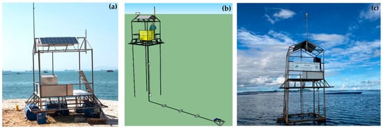
Figure 1. Installation of the GOT001 telemetry station: (a) base structure of the platform without equipment, (b) installation plan of the GOT001 station, and (c) overall view of the GOT001 telemetry station following installation for field deployment.

Table 1. Abbreviations, units, and instrument of meteorological, hydrochemical, and biological parameters measured at the GOT001 station (2020–2024).

Abbreviation	Full Name (Unit)	Instrument/Model
Meteorological parameters
AIRTEMP	Air temperature (°C)	MaxiMet GMX501
DEWPOINT	Dew point temperature (°C)
PRECIP	Precipitation (mm)
PRESSURE	Atmospheric pressure (hPa)
RH	Relative humidity (%)
WINDDIR	Real-time wind direction (degrees)
WINDSPD	Real-time wind speed (m/s)
SOLAR	Solar radiation (W/m2)
Hydrochemical parameters
COND	Electrical conductivity (µS/cm)	Infinity–CTW
SAL	Salinity (PSU)
SEATEMP	Sea surface temperature (°C)
DO	Dissolved oxygen (mg/L)	Rinkow–w (AROW2)
DOSAT	Dissolved oxygen saturation (%)
TURB	Turbidity (NTU)	Infinity–CLW
Hsig	Significant wave height (m)	Nortek AWAC 1 MHz
Hmax	Maximum wave height (m)
CURDIR	Near surface current direction (degrees)
CURSPD	Near surface current speed (m/s)
TP	Top peak wave period (s)
WAVEDIR	Wave direction (degrees)
WLEVEL	Water level (m)
pH	Power of hydrogen	Digital pH sensor
Biological parameter
Chl-a	Chlorophyll-a concentration (µg/L)	Infinity–CLW

2.2. Field Measurement Meteorological, Hydrochemical, and Biological Data

Hourly meteorological, hydrochemical and biological data were recorded at station GOT001 from February 2020 to February 2024. The measured parameters and their corresponding units and instruments are listed in Table 1. A total of approximately 34,715 data points per parameter were obtained over the four-year period, although some gaps occurred due to regular maintenance, instrument recalibration, and repair activities.

2.3. Feature Selection

To identify the most influential predictors of Chl-a, RF model was used, which provides variable-importance estimates based on impurity reduction within decision trees (DT) during training. The importance scores indicated the relative impact of each input on forecast accuracy. The feature selection workflow is summarized (Table 2). The three most important variables associated with Chl-a were selected for subsequent analysis with the hybrid DL model. This selection aimed to simplify the model and reduce processing time without compromising forecasting accuracy, thereby increasing field feasibility. This approach is consistent with prior aquaculture research that used RF to reduce input dimensionality before applying DL techniques [13].

Table 2. Workflow for feature selection using an RF regressor.

Step	Description
Library import	Utilize pandas for data handling and RF Regressor from sklearn for model training, along with additional packages for preprocessing and evaluation.
Data loading and preprocessing	Import data, filter relevant features and target variables, handle missing values.
Train–test split	Partition dataset into training and testing subsets (80/20 split).
Model configuration and training	Initialize the RF with specific parameters (n_estimators = 100, random_state = 42, max_depth = 5, max_leaf_nodes = 10), and fit the model on the training set.
Performance evaluation	Evaluate model accuracy using MAE on both training and testing sets.
Prediction visualization	Generate scatter plots of predicted vs. actual values to assess prediction trends.
Feature importance plot	Create bar plot of feature importance scores to highlight key variables for each prediction target.

2.4. Chl-a Classification for Prediction

The Chl-a classification process comprised data preparation, clustering, and visualization to determine appropriate classes for subsequent analysis.

Chl-a data collected from station GOT001 were gap–filled for missing values (NaN) using forward fill and backward fill to maintain time-series continuity [20]. This procedure was conducted with Pandas 2.3.1 in Python 3.10. The data were classified using two approaches for comparison. In step 1 (quantile-based binning), Chl-a was divided into three classes (low, medium, high) using the pd.qcut function in Pandas, with each class containing approximately the same number of observations. Classes were labeled 1, 2, and 3, respectively, with concentration boundaries determined automatically from the dataset. In step 2 (validation), K-means clustering was applied with three clusters (n_clusters = 3) to align with the quantile-based approach, using the KMeans class in scikit–learn and setting random_state = 42 for reproducibility. Cluster labels were reordered by mean Chl-a concentration from lowest to highest to match the class interpretation (1 = low, 2 = medium, 3 = high). The distribution and class structure of Chl-a were visualized using two plots: a histogram showing the frequency distribution of Chl-a concentrations colored by quantile-based classes, and a box plot showing the distribution within each class (median, interquartile range, and outliers) based on quantile binning (Qcut) [27]. All analyses were conducted in Python 3.10 on Google Colaboratory cloud platform using open-source libraries: Pandas 2.3.1, NumPy 2.0.2, Matplotlib 3.9.1, Seaborn 0.13.2, and scikit–learn 1.5.0.

2.5. CNN–LSTM

The CNN–LSTM framework was designed to integrate spatial feature extraction with temporal sequence modeling for Chl-a prediction (Figure 2). The architecture began with a one-dimensional convolutional layer (1D–CNN) with 1024 filters and a kernel size of 3, using a rectified linear unit (ReLU) activation to capture local temporal patterns. Input dimensions were defined as (Xtrain.shape[1], 1), corresponding to the training sequence length. A max-pooling layer (pool_size = 1) followed to reduce dimensionality while preserving temporal structure. Outputs from the convolutional stage were then passed to an LSTM layer to learn sequential dependencies. Finally, fully connected dense layers with a softmax output unit performed classification into Chl-a risk categories [13].

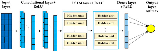
Figure 2. Hybrid CNN–LSTM architecture for Chl-a classification. The framework integrates convolutional and recurrent layers to capture local temporal patterns and sequential dependencies in meteorological, hydrochemical and biological data. The model includes an input layer representing time-series variables, two convolutional layers with ReLU activations for feature extraction and noise reduction, stacked LSTM layers to retain temporal dependencies, a dense layer with ReLU activation to aggregate learned features, and a final softmax output layer to classify Chl-a into ecological risk categories.

2.6. BILSTM

Schuster and Paliwal [28] introduced BiLSTM, extending the LSTM architecture to process information in both forward and backward directions. This bidirectional design allows the network to use information from both past and future time steps to improve predictive performance. Outputs from the forward and backward LSTM are concatenated to form a context-aware representation [29]. The operation of the forward and backward LSTM is shown in Figure 3.

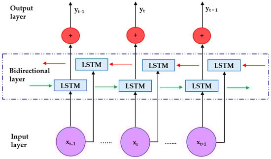
Figure 3. BiLSTM architecture comprising an input layer, a bidirectional layer, and an output layer. Each time step in the input layer (x_t−1, x_t, x_t+1) is fed into both the forward LSTM (green arrows) and the backward LSTM (red arrows). The results from both directions are combined (blue boxes) and then sent to the output layer (y_t−1, y_t, y_t+1), respectively.

2.7. Attention

Attention is a mechanism that helps the model focus on information most relevant for prediction. It assigns weights to time-series locations by comparing the query (Q) and the keys (K) to measure similarity, and then combines the results with the values (V) to produce a context vector that emphasizes important information [30,31]. Here, Q (query) represents the “question” used to find salient information, K (key) serves as the “reference” for each location to match with Q, and V (value) contains the data used to generate the output. This mechanism enhances the model’s ability to capture temporal relationships and improves interpretability. In this study, Attention was combined with CNN and BiLSTM to improve learning from complex temporal data. The basic structure of the Attention mechanism is illustrated in Figure 4, where the attention weight vector W = [W₁, W₂, …, W_n] is multiplied with the values to obtain the fused output.

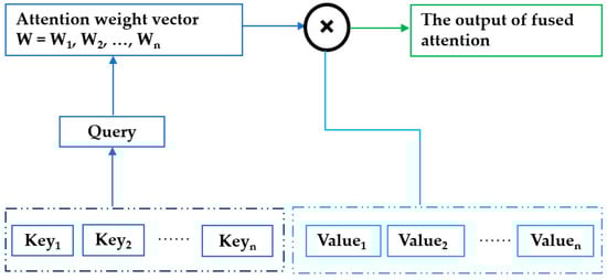
Figure 4. Attention structure, attention mechanism computes a context vector by weighting past observations according to their relevance to the current query. This fused attention vector is used as the input to the prediction layer.

2.8. Data Processing, Analysis, and Visualization

All tasks related to data processing, analysis, and deep learning model development were performed in Python 3.10 on Google Colaboratory. Initial data preparation included Pandas 2.3.1 for data manipulation and restructuring, scikit–learn 1.5.0 for dataset partitioning and scaling with MinMaxScaler, and TensorFlow 2.17.0 for neural network construction and training.

Models were implemented using TensorFlow’s Keras API with the following key layers: Conv1D, MaxPooling1D, Attention, GlobalAveragePooling1D, Dense, Dropout, and the Model class for assembly. In this study, we selected 24 time steps for the CNN–BiLSTM input, corresponding to one full day of hourly measurements, allowing the model to capture daily temporal patterns in environmental parameters while maintaining computational efficiency; for the Conv1D layers, a kernel size of 3 and 64 filters were chosen based on preliminary experiments and prior studies to capture local temporal features efficiently [32,33,34]. Model evaluation used accuracy, precision, recall, and F1 score (Section 2.9), together with scikit–learn’s classification_report and confusion_matrix. Visualization employed Matplotlib 3.9.1 and Seaborn 0.13.2 to produce plots comparing predicted and actual values and to summarize performance (accuracy curves and confusion-matrix heatmaps).

The dataset was split into training (80%) and test (20%) sets using stratified sampling by Chl-a classes. The models evaluated were CNN–LSTM, CNN–BiLSTM, and CNN–BiLSTM–Attention. Training began with 100 epochs, followed by iterative fine-tuning in additional 100-epoch blocks until the mean accuracy no longer improved. Details of the three model configurations are summarized (Table A1).

2.9. Model Performance Evaluation

Model performance was assessed using accuracy, precision, recall, and F1 score. Accuracy is the proportion of correct predictions among all cases; precision is the proportion of correctly identified positive cases among all predicted positives; recall is the proportion of true positives that were correctly identified; and the F1 score is the harmonic mean of precision and recall, providing a single measure that balances both.

2.10. Code Availability

The corresponding authors can provide the full code used for model implementation and analysis upon reasonable request.

3. Results

3.1. Meteorological, Hydrochemical, and Biological Results

The mean and maximum and minimum values of meteorological, hydrochemical, and biological data including AIRTEMP, DEWPOINT, PRECIP, PRESSURE, RH, WINDDIR, WINDSPD, SOLAR, COND, SAL, SEATEMP, DO, DOSAT, TURB, Hsig, Hmax, CURDIR, CURSPD, TP, WAVEDIR, WLEVEL, pH, and Chl-a. The measured values of the various parameters over a 4-year period are shown in Table 3.

Table 3. Summary of data completeness and descriptive statistics for each parameter.

Parameter	Unite	Mean ± Sd	Min	Max
Meteorological parameters
AIRTEMP	°C	28.39 ± 1.85	19.10	33.70
DEWPOINT	°C	25.27 ± 2.35	10.10	29.50
PRECIP	mm	0.16 ± 1.48	0.00	45.60
PRESSURE	hPa	1008.74 ± 2.77	999.10	1017.80
RH	%	83.34 ± 9.13	38.00	100.00
WINDDIR	degrees	162.90 ± 82.54	0.00	359.00
WINDSPD	m/s	3.93 ± 1.83	0.03	15.88
SOLAR	W/m2	219.66 ± 313.90	0.00	1431
Hydrochemical parameters
COND	µS/cm	51.56 ± 4.25	2.84	71.60
SAL	PSU	30.58 ± 2.67	5.14	43.24
SEATEMP	°C	29.85 ± 1.64	23.74	33.89
DO	mg/L	5.97 ± 1.32	0.00	11.95
DOSAT	%	95.50 ± 31.98	0.00	200.00
TURB	NTU	14.90 ± 78.49	0.00	995.89
Hsig	m	0.12 ± 0.10	0.00	2.38
Hmax	m	0.21 ± 0.16	0.02	3.01
CURDIR	degrees	165.75 ± 106.15	0.00	360.00
CURSPD	m/s	0.08 ± 0.05	0.00	0.51
TP	s	3.38 ± 0.98	0.60	33.33
WAVEDIR	degrees	199.36 ± 43.20	0.11	359.91
WLEVEL	m	0.13 ± 0.80	−2.16	2.24
pH	–	–	7.00	9.00
Biological parameter
Chl-a	µg/L	3.79 ± 5.85	0.00	105.42

3.2. Feature Selection and Chl-a Classification Results

Feature selection for Chl-a prediction used meteorological, hydrochemical, and biological data from the first two years of the record, which contained the most complete observations across parameters. The RF regressor showed close agreement between predicted and observed Chl-a within the range of approximately 4.8–5.8 µg/L (Figure 5) and yielded low errors for both the training set (MAE = 0.021) and the test set (MAE = 0.019).

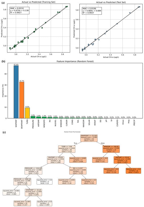
Figure 5. The workflow used for variable screening and feature selection. (a) shows the distribution of observations retained after applying a complete–case analysis, in which only records containing valid measurements for all 23 parameters were preserved. This ensures a consistent data structure and avoids distortions that could arise from imputing missing values, thereby improving the reliability of the feature–selection outcomes. (b) presents the RF variable-importance ranking, highlighting the predictors exerting the strongest influence on Chl-a classification, and (c) displays the distributions of the top contributing variables, illustrating how changes in SEATEMP, DEWPOINT, and TURB correspond to differences among the Chl-a classes.

Variable importance from the RF indicated that relatively few predictors dominated model performance. SEATEMP showed the highest importance with Chl-a 0.474 (47.4%), DEWPOINT 0.327 (32.7%), and TURB 0.095 (9.5%) (Figure 5). Based on these features, Chl-a concentrations were stratified into three ranges using Qcut: Class 1 (0.00–1.45 µg/L), Class 2 (1.45–2.77 µg/L), and Class 3 (2.77–105.42 µg/L). Substantial dispersion in Class 3 associated with bloom events (high–magnitude peaks), reflecting naturally occurring extremes critical for robust classification (Figure 6).

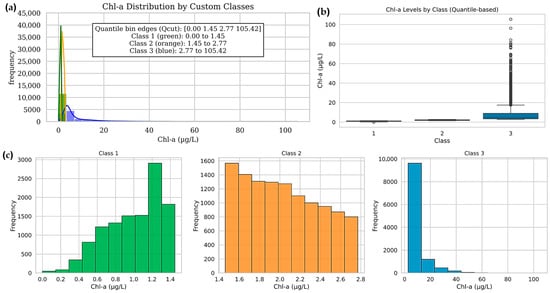
Figure 6. Chl-a classification into three classes using a quantile-based split. (a) histogram showing how the data are distributed across the three Chl-a ranges. (b) the same distribution shown on a linear scale, highlighting the presence of high Chl-a outliers in the upper class, and (c) boxplots comparing the three classes; the upper class displays the widest spread and the highest concentrations.

3.3. Model Performance Results

After fine-tuning, the CNN–LSTM achieved its best performance at 400 epochs with accuracy, precision, recall, and F1 of 0.597 ± 0.006, 0.597 ± 0.180, 0.597 ± 0.006, and 0.593 ± 0.180, respectively, and a processing time of 3.933 ± 0.180 s/step. The CNN–BiLSTM achieved its best performance at 300 epochs with accuracy, precision, recall, and F1 of 0.813 ± 0.012, 0.813 ± 0.012, 0.813 ± 0.012, and 0.813 ± 0.012, respectively, and a processing time of 35.300 ± 1.819 s/step. The CNN–BiLSTM–Attention also achieved its best performance at 300 epochs with accuracy, precision, recall, and F1 of 0.813 ± 0.006, 0.813 ± 0.006, 0.813 ± 0.006, and 0.813 ± 0.006, respectively, and a processing time of 35.510 ± 1.585 s/step. These results are summarized in Table 4.

Table 4. Performance comparison of CNN–LSTM, CNN–BiLSTM, and CNN–BiLSTM–Attention. The highlight shows the best performance of that model.

Model	Epochs Adjusted	Accuracy	Precision	Recall	F1 Score	Time/Step (s)
CNN–LSTM	100	0.573 ± 0.014	0.580 ± 0.017	0.573 ± 0.012	0.570 ± 0.017	3.918 ± 0.354
	200	0.593 ± 0.002	0.597 ± 0.006	0.593 ± 0.006	0.593 ± 0.006	4.031 ± 0.159
	300	0.583 ± 0.020	0.590 ± 0.017	0.573 ± 0.021	0.573 ± 0.021	4.168 ± 0.028
	400	0.597 ± 0.006	0.597 ± 0.180	0.597 ± 0.006	0.593 ± 0.180	3.933 ± 0.180
	500	0.590 ± 0.001	0.600 ± 0.085	0.590 ± 0.085	0.590 ± 0.010	4.029 ± 0.085
	600	0.590 ± 0.002	0.600 ± 0.236	0.590 ± 0.236	0.590 ± 0.000	4.224 ± 0.236
CNN–BiLSTM	100	0.750 ± 0.017	0.750 ± 0.017	0.747 ± 0.023	0.747 ± 0.023	36.997 ± 0.736
	200	0.807 ± 0.006	0.807 ± 0.006	0.807 ± 0.006	0.807 ± 0.006	34.403 ± 1.991
	300	0.813 ± 0.012	0.813 ± 0.012	0.813 ± 0.012	0.813 ± 0.012	35.300 ± 1.819
	400	0.813 ± 0.012	0.820 ± 0.000	0.820 ± 0.000	0.820 ± 0.000	35.733 ± 1.137
	500	0.813 ± 0.006	0.813 ± 0.006	0.813 ± 0.006	0.813 ± 0.006	35.667 ± 1.002
CNN–BiLSTM–Attention	100	0.750 ± 0.017	0.750 ± 0.017	0.750 ± 0.017	0.750 ± 0.017	36.207 ± 0.131
	200	0.807 ± 0.006	0.807 ± 0.006	0.807 ± 0.006	0.807 ± 0.006	36.743 ± 0.649
	300	0.813 ± 0.006	0.813 ± 0.006	0.813 ± 0.006	0.813 ± 0.006	35.510 ± 1.585
	400	0.813 ± 0.006	0.813 ± 0.006	0.810 ± 0.000	0.810 ± 0.000	35.277 ± 1.704
	500	0.813 ± 0.006	0.810 ± 0.000	0.810 ± 0.000	0.810 ± 0.000	34.200 ± 0.300

Figure 7 presents the confusion matrices of the three models and shows how the samples were classified into the three Chl-a classes. From these matrices, Class 3 is generally identified more clearly than the other classes, while most misclassifications occur between Class 1 and Class 2, which have more overlapping characteristics. Based on these results, the class-wise performance metrics are summarized in Figure 8. For the CNN–LSTM model, Class 3 gives the highest values for all four metrics, with accuracy, precision, recall, and F1–score of 80.0%, 72.6%, 64.6%, and 68.3%, respectively. Class 1 shows intermediate performance, whereas Class 2 remains the most difficult class to predict. A similar situation is observed for the CNN–BiLSTM model. Class 3 again shows the best performance, with accuracy of 91.4%, precision of 86.1%, recall of 88.4%, and F1-score of 87.2%. Class 1 ranks second, and Class 2 has the lowest scores. The CNN–BiLSTM–Attention model follows the same class ranking, with Class 3 achieving the highest accuracy (91.4%), precision (88.5%), recall (85.2%), and F1-score (86.8%). While the CNN–BiLSTM and CNN–BiLSTM–Attention models improve class-wise performance compared with CNN–LSTM, this improvement comes with a clear increase in computational cost. The average processing time per step rises from 3.933 ± 0.180 s/step for CNN–LSTM to 35.300 ± 1.819 and 35.510 ± 1.585 s/step for CNN–BiLSTM and CNN–BiLSTM–Attention, respectively (Table 4).

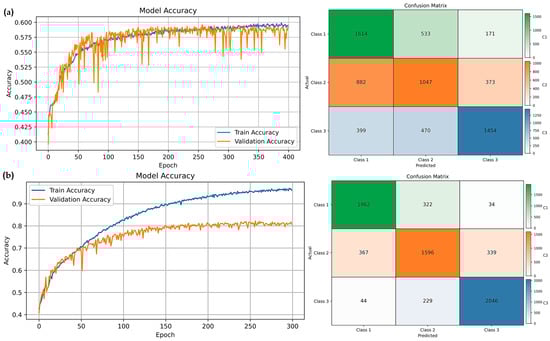
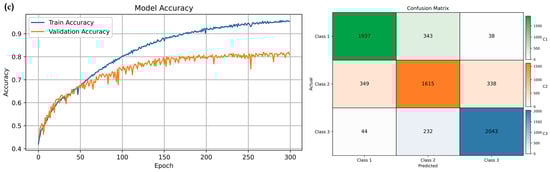
Figure 7. Left: accuracy and loss curves across epochs for the training and validation datasets. Right: confusion-matrix heat maps at the best epoch for test–set Chl-a classes and overall accuracy: (a) CNN–LSTM, (b) CNN–BiLSTM, and (c) CNN–BiLSTM–Attention.

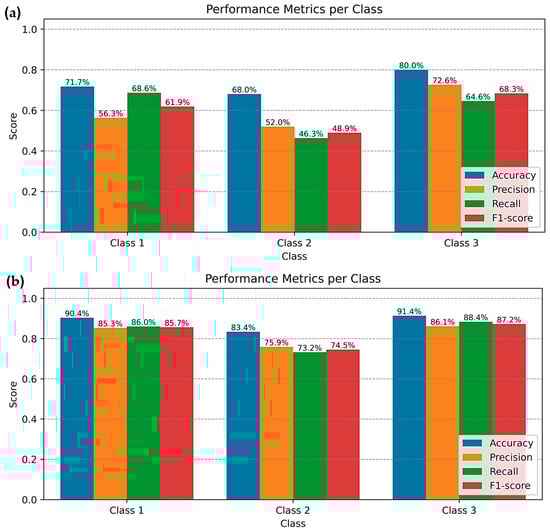
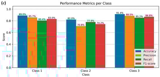
Figure 8. Performance metrics per class, including accuracy, precision, recall, and F1–score, for Chl-a classification obtained from the best fine-tuned models: (a) CNN–LSTM (400 epochs), (b) CNN–BiLSTM (300 epochs), and (c) CNN–BiLSTM–Attention (300 epochs). All metrics are dimensionless ratios by definition; however, they are reported as percentages to facilitate interpretation and comparison across classes. The apparent inconsistency between the class-wise performance ranking in panel (a) and the corresponding confusion matrix in Figure 7a arises from the definition of class-wise accuracy, which is computed using a one-vs-all approach. As a result, this metric reflects not only correctly classified samples of the target class but also true negatives from the remaining classes, rather than relying solely on the diagonal elements of the confusion matrix.

4. Discussion

4.1. Meteorological, Hydrochemical, and Biological Characteristics

Meteorological, hydrochemical, and biological results from the GOT001 station during 2020–2024 have shown seasonal and hourly variability in key variables, including SEATEMP, SAL, DO, and Chl-a. These patterns are consistent with the dynamics of coastal ecosystems in the eastern Gulf of Thailand, which are influenced by monsoons and nutrient inputs from the Chao Phraya and Bang Pakong Rivers, and which directly affect phytoplankton abundance [5]. Consequently, continuous, multi-year, hourly datasets across multiple parameters from GOT001 are valuable for predictive modeling to support coastal aquaculture management and water quality assessment.

4.2. Interpretation of Feature Selection and Chl-a Classification

Variable selection using RF has indicated that SEATEMP, DEWPOINT, and TURB are the most important predictors of Chl-a, together contributing more than 90%, whereas other variables have shown low importance (<0.02). This finding has been consistent with prior research showing that reducing input dimensionality can simplify model implementation without compromising accuracy [13,18,19]. The three variables have also shown clear relationships with Chl-a: SEATEMP affects photosynthesis and oxygen solubility; DEWPOINT, reflecting humidity and near-surface stability, was included because higher moisture reduces latent heat loss, promoting stratification that affects light, nutrients, and Chl-a variability [35,36,37] and TURB reflects suspended solids and nutrient availability that stimulate phytoplankton growth [5].

Chl-a concentrations spanned a broad range in this dataset with 3.79 ± 5.85 µg/L (range: 0–105.42 µg/L), reflecting the natural variability of the coastal system. To interpret this spread in a way that supports classification modeling, the values were divided into three groups using a quantile-based approach (tertiles). This method ensures that each class contains roughly one–third of the observations and represents a statistical rather than ecological partition. Similar low–medium–high groupings have been used in previous studies to support trophic or eutrophication assessment where continuous Chl-a values are discretized for classification tasks [38]. The resulting classes in our study were well separated, with mean Chl-a values increasing progressively from Class 1 to Class 3.

Once categorized, the upper class (Class 3: 2.77–105.42 µg/L) encompassed the range in which many reports have documented phytoplankton bloom development in tropical marine environments. Bloom activity has been recorded at concentrations as low as 3–5 µg/L and may intensify beyond 50–100 µg/L under favorable environmental drivers [6,7,17]. The higher values captured within Class 3 therefore overlap with conditions known to support bloom formation, although the class boundaries themselves should not be interpreted as ecological thresholds. Only the upper portion of Class 3 represents elevated ecological or aquaculture risk, so interpretation should focus on the distribution of these high–end episodes rather than the numerical cutoffs.

4.3. Interpretation of Model Performance

Performance comparisons have shown that CNN–BiLSTM outperformed CNN–LSTM, with mean accuracy of 0.813 (81.3%) versus 0.597 (59.7%). CNN–BiLSTM has also shown stronger performance in predicting the highest Chl-a class, which is critical for monitoring bloom events [30,39]. Adding the Attention mechanism did not increase average accuracy (0.813 ± 0.012 and 0.813 ± 0.006 at 300 epochs), likely because a small set of key variables (SEATEMP, DEWPOINT, TURB) already captured the dominant variability, allowing CNN–BiLSTM to learn temporal relationships without additional weighting. Prior reports have indicated that attention is particularly useful when data are highly complex or when the number of variables is large, improving interpretability and accuracy in those settings [30,40].

The CNN–BiLSTM achieved a maximum accuracy of 81.3%, lower than some previous studies (85–94%) [20,21,22,23,24]. Although 23 parameters were initially measured, only a subset was used after feature selection for model training. The lower accuracy likely reflects both the reduced number of input parameters and the high variability of real-field, hourly data over four years, which capture rapid fluctuations and extreme events not present in monthly or annual datasets [20,22]. In some cases, remote sensing has been used to predict Chl-a, which provides broad spatial coverage but cannot fill gaps when in situ measurements are missing [23], or studies have relied on specific instruments and variables that are not easily substituted [24], or have required many covariates that are difficult to obtain in practice (e.g., 4 variables in [21]; 12 in [20]; 22 in [22]. Although the accuracy here is slightly lower, the approach remains practical because it uses high-frequency, comprehensive field data and relies on SEATEMP, DEWPOINT, and TURB, which are readily measured continuously. Moreover, classifying Chl-a into three levels (low–medium–high) rather than performing daily regression has reduced uncertainty and improved interpretability for risk assessment, early warning, and farm management [15,19], CNN–BiLSTM and CNN–BiLSTM–Attention have required nearly ten times the processing time per step compared with CNN–LSTM, so practical deployment should consider the trade-off between accuracy and computational cost.

4.4. Limitations

This study did not perform data scaling (normalization) because most variables had similar ranges and did not introduce biases that would hinder learning. In addition, RF, CNN, and BiLSTM are relatively robust to scale differences. RF uses threshold-based node splitting that is insensitive to normalization, and CNN–BiLSTM focus on temporal and spatial pattern learning rather than absolute magnitudes. Non-scaling has also allowed straightforward interpretation consistent with water quality benchmarking. The dataset contained a substantial amount of missing data; normalization can introduce computational bias and complicate imputation, whereas using raw values has mitigated these issues. Results (Table 4; Figure 7 and Figure 8) have confirmed that the models could learn effectively and achieve high accuracy without normalization. Therefore, avoiding scaling has been appropriate for this environmental dataset and has supported effective interpretation and practical application.

4.5. Future Work

Future efforts should increase spatial and temporal coverage by integrating data from multiple monitoring stations as the network expands in the Gulf of Thailand. Combining in situ observations with satellite remote sensing or unmanned aerial vehicle (UAV) data should enhance forecasts across larger spatial domains and continuous time scales. More sophisticated hybrid architectures or transfer learning should be developed and tested to better capture spatiotemporal relationships, particularly as the number of input variables increases. Future experiments should explore varying time steps, kernel sizes, and the number of filters in the CNN–BiLSTM model to optimize performance. A near real-time framework should be established to support decision-making for coastal aquaculture, linking models with automated monitoring to provide timely bloom or red-tide warnings. Additionally, defining specific hazard thresholds, particularly for high chlorophyll classes, and exploring short-term predictions (e.g., 72 h ahead) could provide more actionable guidance for aquaculture management. Finally, the approach presented here can be extended to other key water quality parameters, including DO, TAN, NO₂–N, and ALK, to develop an integrated forecasting system for sustainable aquaculture management in coastal areas.

5. Conclusions

This study develops a hybrid CNN–BiLSTM model to classify Chl-a in a coastal ecosystem using high-frequency field data from GOT001 in Si Racha Bay, eastern Gulf of Thailand, during 2020–2024. RF analysis indicates that three key variables—SEATEMP, DEWPOINT, and TURB—serve as effective primary predictors. The CNN–BiLSTM model achieves the highest performance for classifying Chl-a into three levels (low–medium–high), with an average accuracy of 81.3%, substantially higher than CNN–LSTM. Incorporating the attention mechanism does not increase accuracy, likely because the limited but highly informative predictors (SEATEMP, DEWPOINT, TURB) already capture the dominant variability. These findings support the feasibility of using parsimonious, computationally efficient models to build near-real-time Chl-a forecasting systems for coastal aquaculture management, algal-bloom or red-tide warning, and ecological risk assessment. The approach is extensible to other water-quality parameters, including DO, TAN, NO₂–N, and ALK, to develop an integrated monitoring and forecasting system that supports the sustainable management of coastal aquaculture farms.

References

- Willer, D.F.; Robinson, J.P.W.; Patterson, G.T.; Luyckx, K. Maximising sustainable nutrient production from coupled fisheries–aquaculture systems. PLoS Sustain. Transform. 2022, 1, e0000005. [Google Scholar] [CrossRef]
- Trujillo, P.; Piroddi, C.; Jacquet, J. Fish farms at sea: The ground truth from Google Earth. PLoS ONE 2012, 7, e30546. [Google Scholar] [CrossRef]
- Food and Agriculture Organization (FAO). The State of World Fisheries and Aquaculture 2020; FAO: Rome, Italy, 2020; Available online: https://www.fao.org/documents/card/en/c/ca9229en (accessed on 10 August 2025).
- Deng, J.; Chen, F.; Hu, W.; Lu, X.; Xu, B.; Hamilton, D.P. Variations in the distribution of Chl-a and simulation using a multiple regression model. Int. J. Environ. Res. Public Health 2019, 16, 4553. [Google Scholar] [CrossRef] [PubMed]
- Luang-on, J.; Ishizaka, J.; Buranapratheprat, A.; Phaksopa, J.; Goes, J.I.; Kobayashi, H.; Hayashi, M.; Maúre, E.D.R.; Matsumura, S. Seasonal and interannual variations of MODIS-Aqua chlorophyll-a (2003–2017) in the upper Gulf of Thailand influenced by Asian monsoons. J. Oceanogr. 2022, 78, 209–228. [Google Scholar] [CrossRef]
- Heisler, J.; Glibert, P.M.; Burkholder, J.M.; Anderson, D.M.; Cochlan, W.; Dennison, W.C.; Dortch, Q.; Gobler, C.J.; Heil, C.A.; Humphries, E.; et al. Eutrophication and harmful algal blooms: A scientific consensus. Harmful Algae 2008, 8, 3–13. [Google Scholar] [CrossRef] [PubMed]
- Paerl, H.W.; Otten, T.G. Harmful cyanobacterial blooms: Causes, consequences, and controls. Microb. Ecol. 2013, 65, 995–1010. [Google Scholar] [CrossRef]
- Bresciani, M.; Stroppiana, D.; Odermatt, D.; Morabito, G.; Giardino, C. Assessing remotely sensed chlorophyll-a for the implementation of the Water Framework Directive in European perialpine lakes. Sci. Total Environ. 2011, 409, 3083–3091. [Google Scholar] [CrossRef]
- Reynolds, C.S. The Ecology of Phytoplankton; Cambridge University Press: Cambridge, UK, 2006. [Google Scholar] [CrossRef]
- Huisman, J.; Codd, G.A.; Paerl, H.W.; Ibelings, B.W.; Verspagen, J.M.H.; Visser, P.M. Cyanobacterial blooms. Nat. Rev. Microbiol. 2018, 16, 471–483. [Google Scholar] [CrossRef]
- Gons, H.J.; Auer, M.T.; Effler, S.W. MERIS satellite chlorophyll mapping of oligotrophic and eutrophic waters in the Laurentian Great Lakes. Remote Sens. Environ. 2008, 112, 4098–4106. [Google Scholar] [CrossRef]
- Cloern, J.E.; Foster, S.Q.; Kleckner, A.E. Phytoplankton primary production in the world’s estuarine–coastal ecosystems. Biogeosciences 2014, 11, 2477–2501. [Google Scholar] [CrossRef]
- Jongjaraunsuk, R.; Taparhudee, W.; Suwannasing, P. Comparison of water quality prediction for red tilapia aquaculture in an outdoor recirculation system using deep learning and a hybrid model. Water 2024, 16, 907. [Google Scholar] [CrossRef]
- Jongjaraunsuk, R.; Taparhudee, W. Optimizing prediction of key water quality parameters in tilapia river-based cage culture using simple parameters based on different deep learning models. Agric. Nat. Resour. 2025, 59, 590412. [Google Scholar] [CrossRef]
- Palani, S.; Liong, S.Y.; Tkalich, P. An ANN application for water quality forecasting. Mar. Pollut. Bull. 2008, 56, 1586–1597. [Google Scholar] [CrossRef] [PubMed]
- Ahmed, U.; Mumtaz, R.; Anwar, H.; Shah, A.A.; Irfan, R.; García-Nieto, J. Efficient water quality prediction using supervised machine learning. Water 2019, 11, 2210. [Google Scholar] [CrossRef]
- Liu, P.; Wang, J.; Sangaiah, A.K.; Xie, Y.; Yin, X. Analysis and prediction of water quality using LSTM deep neural networks in the IoT environment. Sustainability 2019, 11, 2058. [Google Scholar] [CrossRef]
- Castrillo, M.; López García, A. Estimation of high-frequency nutrient concentrations from water quality surrogates using machine learning methods. Water Res. 2020, 172, 115490. [Google Scholar] [CrossRef]
- Zambrano, A.F.; Giraldo, L.F.; Quimbayo, J.; Medina, B.; Castillo, E. Machine learning for manually measured water quality prediction in fish farming. PLoS ONE 2021, 16, e0256380. [Google Scholar] [CrossRef]
- Kim, H.R.; Soh, H.Y.; Kwak, M.T.; Han, S.H. Machine learning and multiple-imputation approaches to predict chlorophyll-a concentration in the coastal zone of Korea. Water 2022, 14, 1862. [Google Scholar] [CrossRef]
- Barzegar, R.; Aalami, M.T.; Adamowski, J. Short-term water quality variable prediction using a hybrid CNN–LSTM deep learning model. Stoch. Environ. Res. Risk Assess. 2020, 34, 415–433. [Google Scholar] [CrossRef]
- Abbas, A.; Park, M.; Baek, S.S.; Cho, K.H. Deep learning–based algorithms for long-term prediction of chlorophyll-a in catchment streams. J. Hydrol. 2023, 626, 130240. [Google Scholar] [CrossRef]
- Yao, L.; Wang, X.; Zhang, J.; Yu, X.; Zhang, S.; Li, Q. Prediction of sea surface chlorophyll-a concentrations based on deep learning and time-series remote sensing data. Remote Sens. 2023, 15, 4486. [Google Scholar] [CrossRef]
- Huang, C.; Xu, S.; Bi, R.; Jiang, B.; Du, Y.; Ma, H. Chlorophyll-a inversion algorithm and algae classification technique based on hyperspectral data. In Proceedings of the 2024 12th International Conference on Agro-Geoinformatics, Novi Sad, Serbia, 15–18 July 2024; IEEE: Piscataway, NJ, USA, 2024; pp. 1–4. [Google Scholar] [CrossRef]
- Ni, J.; Liu, R.; Tang, G.; Xie, Y. An improved attention-based bidirectional LSTM model for cyanobacterial bloom prediction. Int. J. Control Autom. Syst. 2022, 20, 3445–3455. [Google Scholar] [CrossRef]
- Yu, W.; Wang, X.; Jiang, X.; Zhao, R.; Zhao, S. A novel hybrid model based on two-stage data processing and machine learning for forecasting chlorophyll-a concentration in reservoirs. Environ. Sci. Pollut. Res. 2024, 31, 262–279. [Google Scholar] [CrossRef] [PubMed]
- Mertens, S.; Verbraeken, L.; Sprenger, H.; Demuynck, K.; Maleux, K.; Cannoot, B.; De Block, J.; Maere, S.; Nelissen, H.; Bonaventure, G.; et al. Proximal hyperspectral imaging detects diurnal and drought-induced changes in maize physiology. Front. Plant Sci. 2021, 12, 640914. [Google Scholar] [CrossRef] [PubMed]
- Schuster, M.; Paliwal, K.K. Bidirectional recurrent neural networks. IEEE Trans. Geosci. Remote Sens. 1997, 45, 2673–2681. [Google Scholar] [CrossRef]
- Ihianle, I.K.; Nwajana, A.O.; Ebenuwa, S.H.; Otuka, R.I.; Owa, K.; Orisatoki, M.O. A deep learning approach for human activities recognition from multimodal sensing devices. IEEE Access 2020, 8, 179028–179038. [Google Scholar] [CrossRef]
- Chen, H.; Yang, J.; Fu, X.; Zheng, Q.; Song, X.; Fu, Z.; Wang, J.; Liang, Y.; Yin, H.; Liu, Z.; et al. Water quality prediction based on LSTM and attention mechanism: A case study of the Burnett River, Australia. Sustainability 2022, 14, 13231. [Google Scholar] [CrossRef]
- Shen, T.; Zhou, T.; Long, G.; Jiang, J.; Pan, S.; Zhang, C. DiSAN: Directional self-attention network for RNN/CNN-free language understanding. In Proceedings of the Thirty-Second AAAI Conference on Artificial Intelligence, New Orleans, LA, USA, 2–7 February 2018; pp. 5045–5052. [Google Scholar]
- Wang, C.; Li, X.; Shi, Y.; Jiang, W.; Song, Q.; Li, X. Load forecasting method based on CNN and extended LSTM. Energy Rep. 2024, 12, 2452–2461. [Google Scholar] [CrossRef]
- Tang, W.; Long, G.; Liu, L.; Zhou, T.; Blumenstein, M.; Jiang, J. Omni-Scale CNNs: A simple and effective kernel size configuration for time series classification. In Proceedings of the International Conference on Learning Representations (ICLR), Virtual, 25–29 April 2022. [Google Scholar]
- Lang, C.; Steinborn, F.; Steffens, O.; Lang, E.W. Electricity load forecasting—An evaluation of simple 1D CNN network structures. arXiv 2019. [Google Scholar] [CrossRef]
- Thoppil, P.G. Enhanced phytoplankton bloom triggered by atmospheric high-pressure systems over the northern Arabian Sea. Sci. Rep. 2023, 13, 769. [Google Scholar] [CrossRef]
- Somavilla, R.; Rodriguez, C.; Lavín, A.; Viloria, A.; Marcos, E.; Cano, D. Atmospheric control of deep chlorophyll maximum development. Geosciences 2019, 9, 178. [Google Scholar] [CrossRef]
- Song, H.; Ji, R.; Stock, C.; Kearney, K.; Wang, Z. Interannual variability in phytoplankton blooms and plankton productivity over the Nova Scotian Shelf and in the Gulf of Maine. Mar. Ecol. Prog. Ser. 2011, 426, 105–118. [Google Scholar] [CrossRef]
- Cairo, C.; Barbosa, C.; Lobo, F.; Novo, E.; Carlos, F.; Maciel, D.; Flores Júnior, R.; Silva, E.; Curtarelli, V. Hybrid chlorophyll-a algorithm for assessing trophic states of a tropical Brazilian reservoir based on Sentinel-2 MSI data. Remote Sens. 2020, 12, 40. [Google Scholar] [CrossRef]
- Cai, H.; Zhang, C.; Xu, J.; Wang, F.; Xiao, L.; Huang, S.; Zhang, Y. Water quality prediction based on the KF-LSTM encoder–decoder network: A case study with missing data collection. Water 2023, 15, 2542. [Google Scholar] [CrossRef]
- Ehteram, M.; Ahmed, A.N.; Sherif, M.; El-Shafie, A. An advanced deep learning model for predicting the water quality index. Ecol. Indic. 2024, 160, 111806. [Google Scholar] [CrossRef]
Disclaimer/Publisher’s Note: The statements, opinions and data contained in all publications are solely those of the individual author(s) and contributor(s) and not of MDPI and/or the editor(s). MDPI and/or the editor(s) disclaim responsibility for any injury to people or property resulting from any ideas, methods, instructions or products referred to in the content. |
© 2025 by the authors. Licensee MDPI, Basel, Switzerland. This article is an open access article distributed under the terms and conditions of the Creative Commons Attribution (CC BY) license.