An Enhanced Machine Learning Approach for Regional Total Suspended Matter Concentration Retrieval Using Multispectral Imagery

Abstract

Accurate monitoring of total suspended matter (TSM) concentration is essential for aquatic ecosystem protection and water quality assessment. Multispectral remote sensing provides an effective approach for large-scale TSM monitoring. However, robust retrieval models are difficult to develop due to limited in situ data. This study presents a Deep Feature Extraction–Machine Learning fusion framework that integrates a pre-trained back-propagation neural network (BPNN) with support vector regression (SVR) to enhance TSM retrieval. High-level spectral features extracted by BPNN are used as inputs to SVR (termed DFE-SVR) for regional TSM retrieval, using in situ measurements from five inland lakes in Jiangsu and Anhui Provinces, China. The generated TSM maps showed spatial patterns consistent with TSM concentration distributions visually observed in true-color imagery. Validation results demonstrated that DFE-SVR outperformed BPNN and SVR models, achieving R² of 0.85 and 0.90 and RMSE of 7.95 and 4.76 mg/L for GF-1 and Sentinel-2 imagery, respectively. Compared with SVR models using principal component analysis or band combinations, DFE-SVR reduced RMSE by over 20%. Under reduced training samples, the DFE-SVR model also maintained higher stability and accuracy. These findings showed its potential for multispectral water quality monitoring with limited in situ data.

1. Introduction

Water quality monitoring is essential for maintaining the health of aquatic ecosystems and ensuring the safety of human water use [1,2]. The concentration of Total Suspended Matter (TSM), a key parameter in water quality assessment, comprises organic and inorganic particles (e.g., sediments and phytoplankton) suspended in the water column [3,4,5,6]. Its concentration directly influences light penetration, primary productivity, and the overall health of aquatic ecosystems [7,8,9,10,11]. Therefore, efficiently and accurately retrieving TSM spatiotemporal dynamics is crucial for aquatic ecosystem protection and water quality evaluation.

Traditional methods of measuring TSM involve in situ sampling and laboratory analysis, which, although accurate, are costly and limited in spatial and temporal coverage [12,13]. Remote sensing provides an effective approach to monitor TSM and its spatiotemporal changes at regional and watershed scales [14]. This is achieved by modeling the relationship between the water constituents’ concentrations and scattering signals (i.e., water-leaving radiance) from the sensors [15]. Multispectral and hyperspectral sensors have been successfully and widely used in TSM retrieval. Zhang et al. [5] employed Landsat imagery to map the TSM concentrations in Gaoyou Lake over four decades. E. Bubnova et al. [16] estimated the TSM concentrations in the southeastern Baltic Sea from in situ measurements and MODIS-Aqua satellite data for 2003–2016. Friedmann et al. [17] leveraged data fusion of Landsat/Sentinel-2 and MODIS to develop a high-resolution global TSM model. Compared to hyperspectral techniques, multispectral remote sensing remains the most widely adopted owing to its broader coverage, frequent revisits, and easy access.

Empirical [18,19], semi-analytical [20,21], and bio-optical models [22] have traditionally been employed to interpret remote sensing data for water quality parameters assessment. Xie et al. [23] developed an empirical model to retrieve TSM in Nanyi Lake using in situ measurements and synchronous Sentinel-3 OLCI imagery from 2018 to 2022. Zhu et al. [24] inverted a radiative transfer model using spectral reflectance data and a semi-analytical algorithm, achieving a coefficient of determination (R²) of 0.88 for inland waters. However, the substantial optical heterogeneity of water bodies complicates TSM retrieval, as factors including water depth and constituent concentrations markedly influence spectral responses [25,26]. These traditional methods suffer from limited generalization or strong sensitivity to input parameters and atmospheric correction accuracy, severely limiting their application to optically complex waters [27]. In recent years, machine learning has increasingly emerged as a key approach for TSM retrieval, owing to its nonlinear modeling capability, demonstrating higher accuracy and adaptability in heterogeneous and optically complex waters [16,28,29,30]. Liu et al. [12] evaluated multiple machine learning algorithms, including random forest (RF) and genetic algorithm-optimized RF, for TSM retrieval in shallow lakes, achieving high accuracy with R² exceeding 0.98. Wang et al. [31] utilized RF and neural networks to analyze long-term MODIS data for water quality parameters, including TSM, with models achieving R² above 0.89. Fang et al. [32] employed a RF model to estimate the monthly suspended sediment concentration in the Yichang-Chenglingji River section downstream of the Three Gorges Dam. Kupssinskü et al. [33] developed an artificial neural network for TSM retrieval from Sentinel-2 images that attained an R² of 0.7.

Despite the advantages of machine learning approaches, the generalization and robustness of TSM retrieval models are challenged by several practical constraints [34]. The high cost and logistical difficulty of collecting in situ TSM measurements and synchronized spectral data coinciding with satellite overpasses limit the amount of data obtainable in a single campaign, particularly when covering large water bodies [35]. Establishing an accurate relationship between the spectral characteristics and TSM concentrations is essential [28]. However, the effectiveness of machine learning-based models in multispectral TSM retrieval is often hampered by the limited feature representation capacity of multispectral imagery [36]. Moreover, compared to hyperspectral data, multispectral data have fewer bands and exhibit lower sensitivity to TSM variations, necessitating more advanced feature extraction from the available spectral information. Most existing studies rely on shallow feature engineering techniques, such as band combinations [5] or principal component analysis [37], which are often insufficient for capturing the complex nonlinear spectral patterns associated with TSM. In contrast, neural networks can autonomously learn high-level abstract features, overcoming the limitations of hand-crafted features [28]. Nevertheless, their performance heavily depends on the availability of large-scale labeled datasets, rendering them susceptible to overfitting when training samples are limited [38,39]. Therefore, enhancing the ability of retrieval models to characterize the relationship between spectral reflectance and TSM concentrations under limited samples remains a crucial challenge in multispectral-based TSM retrieval.

To address this issue, this study proposes a framework that integrates deep feature extraction and machine learning (DFE-ML). This framework utilizes a pre-trained deep network to extract high-dimensional representations from multispectral reflectance data and integrates a traditional machine learning method for regression modeling, aiming to capitalize on the advantages of artificial neural network models in feature representation while maintaining the robustness of machine learning methods under limited samples.

2. Materials and Methods

2.1. Materials

2.1.1. Study Area and In Situ Data

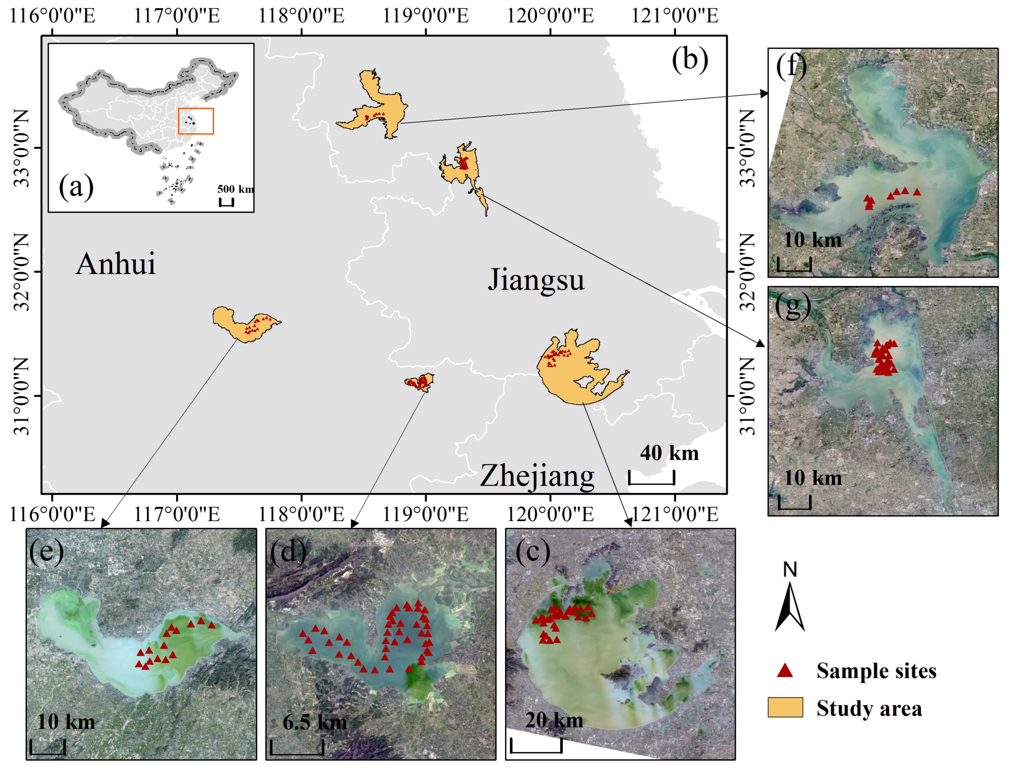
The in situ data were obtained from the 2nd Gaofen Satellite Application Innovation Technology Competition (GFSAIT, https://www.cpeos.org.cn/GFSAIT2024 (accessed on 30 September 2024)) organized by the Earth Observation System & Data Center of China National Space Administration. It included measurements collected at 108 sampling sites, consisting of TSM data and concomitant remote sensing images from Gaofen (GF) satellites. The sampling sites were distributed across five typical inland lakes, including Taihu, Hongze, Gaoyou, Chaohu, and Nanyi, which are located in Jiangsu province and Anhui province (Figure 1). Taihu Lake, the third largest freshwater lake in China, is located at the border of Jiangsu and Zhejiang Provinces, with a surface area of 2338 km² and an average depth of 1.9 m. It is a shallow eutrophic lake that suffers from severe eutrophication due to intensive human activities and frequent wind-induced resuspension of sediments [40]. Hongze Lake, the fourth largest freshwater lake in China, is situated in the lower reaches of the Huai River in western Jiangsu Province, with an average depth of 1.77 m. The lake is characterized by high turbidity and large seasonal variations in suspended matter due to frequent water exchange (approximately every 35 days) and strong monsoon-driven waves [41]. Gaoyou Lake, the third largest lake in Jiangsu Province, lies in the central part of the province along the lower reaches of the Huai River, with an average depth of 1.44 m. It occupies a shallow alluvial depression and is sometimes referred to as a “suspended” lake because its lakebed elevation is higher than the surrounding floodplain, which historically made it prone to embankment breaches and flooding [42]. Chaohu Lake, located in central Anhui Province, is one of China’s five largest freshwater lakes. Covering about 760 km² with an average depth of 3 m, it lies between the Yangtze and Huaihe River basins and is highly susceptible to nutrient pollution and eutrophication [43]. Nanyi Lake, the largest lake in southern Anhui Province, connects to the Shuiyang River and plays a vital ecological role in maintaining regional hydrological stability. However, increasing agricultural and aquacultural activities, as well as domestic sewage discharge, have caused elevated suspended matter concentrations and localized water quality degradation in recent years [44]. These lakes provide a representative spectrum of conditions, ensuring a rigorous assessment of our model’s performance across different sediment types and water color patterns.

Figure 1. Distribution of in situ sampling sites and the study area. (a) Overview of the study area; (b) Locations of the five lakes; (c) Taihu Lake; (d) Nanyi Lake; (e) Chaohu Lake; (f) Hongze Lake; (g) Gaoyou Lake.

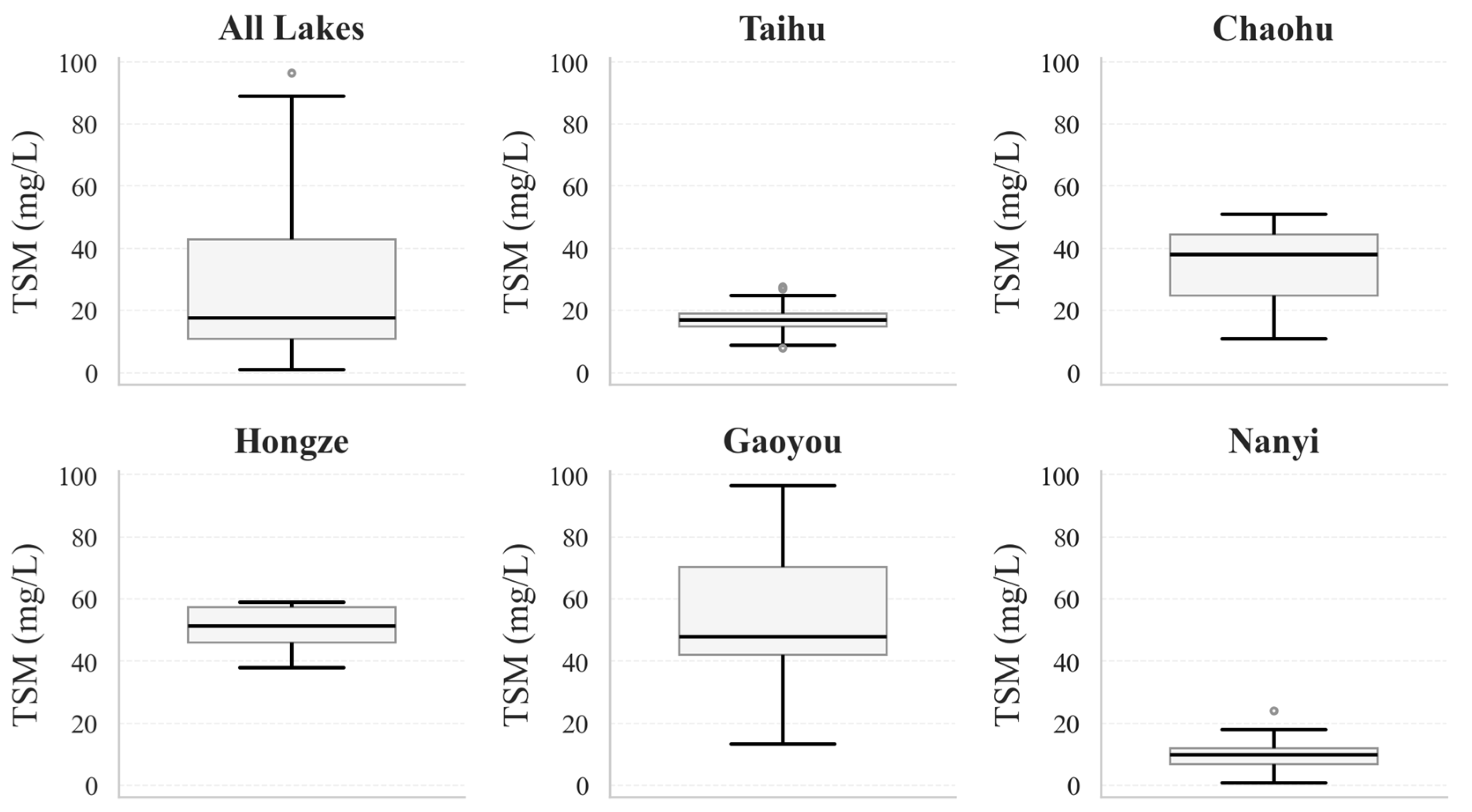
As indicated by the red points in Figure 1, the sampling sites were distributed across five lakes with varying environmental characteristics. In Nanyi Lake, the sites were relatively evenly distributed, while in the larger lakes, the sampling points were strategically located in key zones such as the lake center, river inlets, nearshore areas, and regions with different water depths and turbidity levels. This spatial arrangement ensures that the collected TSM measurements capture the major spatial variability within each lake. The in situ TSM concentrations as measured using the gravimetric method according to the standard method (ISO 1190-89, equivalent to GB 1190-89). The in situ TSM concentrations across the dataset ranged from 1.0 to 96.5 mg/L, with a mean and standard deviation of 27.6 ± 21.3 mg/L. Considerable variations were observed among the lakes, with Hongze Lake (50.7 ± 7.7 mg/L) and Gaoyou Lake (54.6 ± 18.2 mg/L) showing relatively high concentrations, while Nanyi Lake (10.2 ± 4.3 mg/L) and Taihu Lake (17.4 ± 5.0 mg/L) exhibited much lower levels. Chaohu Lake displayed intermediate concentrations, with a mean of 34.3 ± 13.2 mg/L. The boxplots in Figure 2 illustrated the variability and distribution patterns of TSM concentrations both overall and across individual lakes.

Figure 2. Box plots of in situ TSM concentrations for all samples and for individual lakes.

2.1.2. Satellite Imagery and Preprocessing

The GF satellite data, provided by GFSAIT, consisted of 15 scenes of GF-1 imagery and one scene of GF-6 imagery. To further evaluate the applicability of the proposed framework across different sensors, Sentinel-2 data matching the sampling dates were downloaded from the Copernicus Open Access Hub of the European Space Agency (ESA). The sampling and imagery details for the five lakes are presented in Table 1.

Table 1. In situ TSM measurements and corresponding satellite images for the five lakes.

Lake Name	In Situ Sampling Date(s)	Number of In Situ Sites	Number of GF Scenes	Number of Sentinel-2 Scenes
Taihu	17 October 2023	25	3	2
	16 May 2024
Chaohu	1 November 2023	15	1	4
Hongze	23 October 2023	8	6	2
Gaoyou	14 October 2023	25	3	2
	24 May 2024
Nanyi	30 October 2023	35	3	3
	15 October 2023
	8 May 2024

GF-1 imagery, comprising four bands at 16 m spatial resolution, was provided as Level-1 products and preprocessed using ENVI 5.3 software. Images were radiometrically calibrated to radiance and atmospheric corrections were performed using the Fast Line-of-sight Atmospheric Analysis of Hypercubes (FLAASH) method and orthorectification was conducted using Landsat imagery as a reference to ensure geometric fidelity. Sentinel-2 imagery contains 13 bands, with B2 (blue), B3 (green), B4 (red), and B8 (near-infrared) at 10 m spatial resolution, and the remaining bands at 20 m or 60 m. The downloaded data were Level-2A products, which were directly applicable to retrieval. Using the SNAP 13.0.0 software provided by ESA, all bands were resampled to a uniform spatial resolution of 10 m. Bands B1, B9, and B10 were excluded from the analysis during developing the TSM retrieval model, given their primary sensitivity to aerosols and water vapor. These sensor-specific preprocessing workflows were designed to generate consistent, surface reflectance data for each satellite system, thereby minimizing the effects of radiometric, atmospheric, and spatial variations prior to feature extraction and model development.

The in situ TSM measurements were paired with remote sensing reflectance values extracted from corresponding satellite imagery by matching the geographic location and acquisition date of each sample. To ensure data quality, a maximum temporal window of seven days was allowed between the field measurements and the satellite overpasses. Additionally, images with cloud cover or other quality issues were excluded. As a single sampling site could match multiple clear-sky images, a total of 186 and 153 valid sample pairs were obtained for GF-1 and Sentinel-2 sensors, respectively. These sample pairs were then divided into training, validation, and test sets in a ratio of 6:2:2 using stratified random sampling. The stratification was conducted based on the lakes and the range of TSM concentrations to ensure representative distribution across all subsets. In this study, the training set was used for model training, while the validation set was employed to evaluate model performance under different hyperparameter configurations to identify the optimal hyperparameter combination. Finally, the test set was used to assess the accuracy of different models.

2.2. DFE-ML Framework for TSM Retrieval

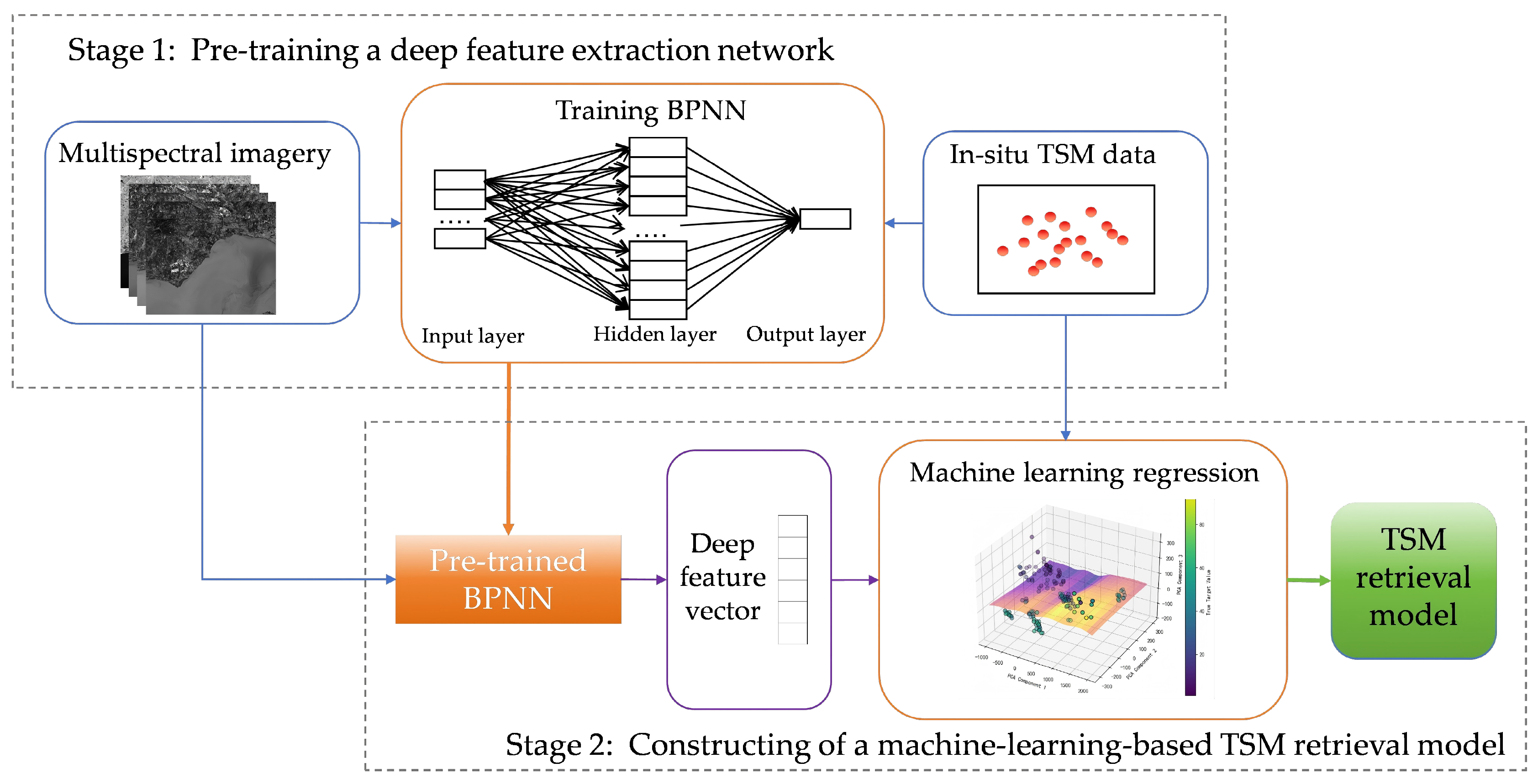
The proposed DFE-ML framework comprises two main stages: (1) pre-training a deep feature extraction network and (2) constructing a machine-learning-based TSM retrieval model (Figure 3).

Figure 3. Overall workflow of the proposed DFE-ML framework.

2.2.1. Pre-Training of a Deep Feature Extraction Network

This stage aims to transform multispectral reflectance data into more discriminative feature representations. Reflectance values from all spectral bands were fed as input into a pre-trained neural network. The reflectance inputs were derived from visible to near-infrared bands that are known to be sensitive to variations in TSM [45,46]. Specifically, shorter wavelengths (blue-green region) are affected by light absorption and scattering from fine inorganic particles, whereas longer wavelengths (red-NIR) are primarily influenced by coarse sediments and organic matter. These physically based sensitivities support the inclusion of all available bands as inputs to the deep feature extractor, enabling it to capture the full range of TSM-related optical responses. Then, the output activation vector from the hidden layer was extracted as fused spectral features. This nonlinear mapping transforms the original spectral information into a higher-dimensional feature space, thereby enhancing its representational capacity and providing more effective inputs for subsequent retrieval modeling.

The backpropagation neural network (BPNN) method was employed in this study, as it is currently one of the most widely used artificial neural networks [47]. The network architecture consisted of an input layer (with the number of neurons corresponding to the number of bands, e.g., 4 for GF-1 and 10 for Sentinel-2), a hidden layer with 64 neurons, and a single-neuron output layer for TSM prediction. The hidden layer employed the Rectified Linear Unit (ReLU) activation function, and the network was trained for 2000 epochs using the Adam optimization algorithm. The initial learning rate was set at 0.1 and reduced to 0.01 after 70 epochs to ensure stable convergence. This configuration was designed to achieve a balance between model expressiveness and computational efficiency. The number of hidden units was determined through preliminary experiments to mitigate overfitting under limited sample conditions. The use of the ReLU activation function and Adam optimizer with a decaying learning rate is standard practice that enhances training stability and accelerates convergence.

The BPNN method was first trained in a supervised manner, using all bands as input and in situ TSM measurements as the target outputs, thereby yielding an initial retrieval model. The pre-trained BPNN model was then applied to extract the 64-dimensional hidden layer representations, which served as the fused spectral features, while its direct TSM predictions were excluded from subsequent steps.

2.2.2. Constructing a Machine-Learning-Based TSM Retrieval Model

Given that ML algorithms such as Support Vector Machines (SVM) and RF have been demonstrated to be more suitable than neural networks for analyzing a small number of samples [48], they were employed in this stage. The extracted deep features served as input variables for machine learning retrieval, with in situ TSM measurements as the target variable. This step utilizes the advantages of machine learning in limited sample learning to build a robust mapping from the feature space to TSM concentration.

In this study, SVR was selected as the regression algorithm owing to its widely acknowledged performance in modeling with limited data [49]. The resulting TSM retrieval model developed under this framework was named DFE-SVR. It was noted that both the feature extraction (via BPNN) and the final regression (via SVR) components of the proposed framework were developed and optimized on the same dataset.

2.3. Evaluation Metrics

To evaluate the performance of the retrieval models, an accuracy assessment was conducted using an independent test set that was not involved in model training. Three widely used statistical metrics were employed, including mean absolute error (MAE), root mean square error (RMSE), and R² [50,51,52]. The evaluation employed R² and RMSE, in line with common practice in TSM estimation [32], while MAE was also incorporated for its lower sensitivity to extreme values, thus offering a more accurate representation of average error [43].

As defined in Equation (1), MAE quantifies the average absolute deviation between predicted and observed TSM concentration:

$$\mathrm{M}\mathrm{A}\mathrm{E}={\displaystyle \frac{1}{\mathrm{n}}}{\sum }_{i=1}^n\left|y_i-{\widehat{y}}_i\right|,$$

(1)

RMSE, given in Equation (2), is sensitive to the magnitude of both large and small errors and reflects the overall accuracy of the predictions:

$$\mathrm{R}\mathrm{M}\mathrm{S}\mathrm{E}=\sqrt{{\displaystyle \frac{1}{\mathrm{n}}}{\sum }_{i=1}^n{\left(y_i-{\widehat{y}}_i\right)}^2},$$

(2)

$R^2$, as shown in Equation (3), explains the proportion of variance in the observed data that can be explained by the model, ranging from 0 to 1, with higher values indicating a better fit:

$$R^2 = 1-{\displaystyle \frac{{\sum }_{i=1}^n{\left(y_i-{\widehat{y}}_i\right)}^2}{{\sum }_{i=1}^n{\left(y_i-\overline{y_i}\right)}^2}},$$

(3)

In general, lower MAE and RMSE values, together with a higher $R^2$, indicate better retrieval performance of the model.

3. Results

3.1. Results of TSM Retrieval

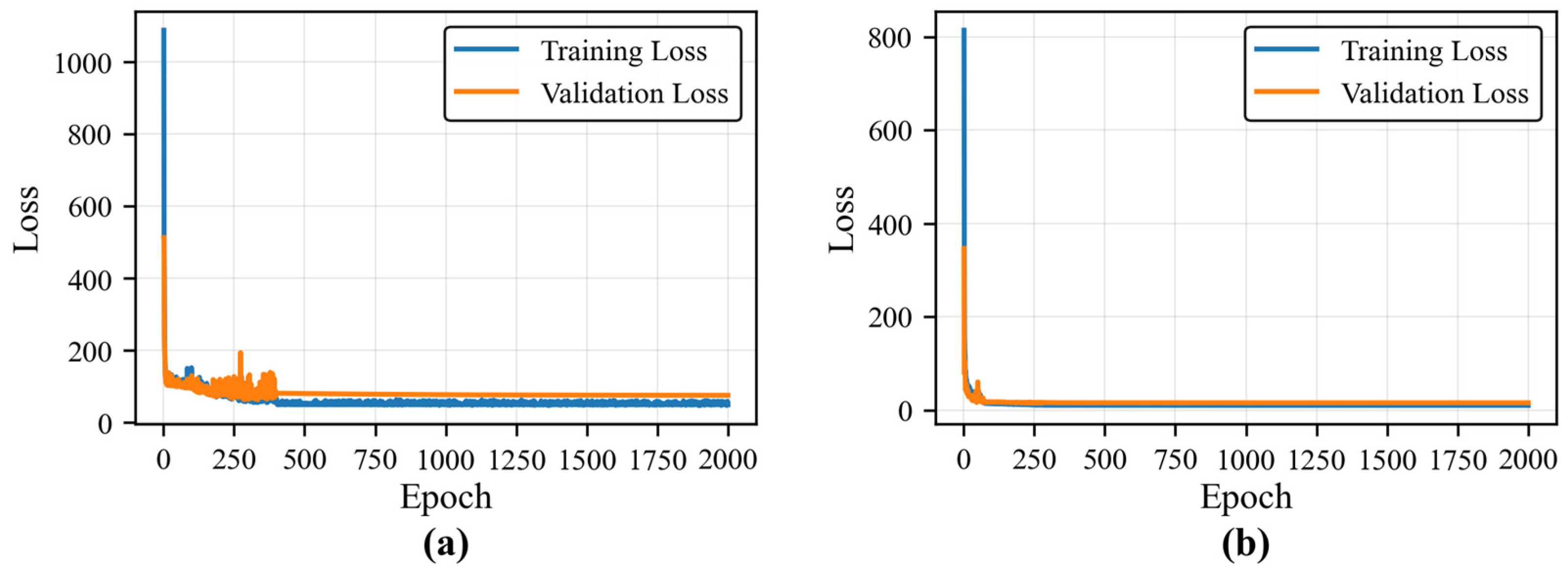
Under the DFE-ML framework, TSM concentrations were retrieved in two main stages. In the first stage, a BPNN model was trained using multispectral reflectance data with the detailed configuration provided in the Section 2.2.1. As illustrated in Figure 4, both the training and validation loss decreased rapidly during the initial phase (epochs 0–50). For the GF-1 data, the training loss stabilized after 1000 epochs, while for Sentinel-2 data, convergence occurred more quickly, with stabilization after around 300 epochs. The trained BPNN model was then used to extract 64-dimensional feature vectors from the hidden layer, which were employed in the second stage. In the second stage, these deep features were input into an SVR model to construct the final TSM retrieval model. Hyperparameters of the SVR model were optimized using a three-fold cross-validation combined with a randomized grid search. The resulting DFE-SVR model was used for TSM retrieval, with in situ TSM measurements as the target variable.

Figure 4. Training process of the BPNN-based models: (a) Training loss curve for the GF-1 data; (b) Training loss curve for the Sentinel-2 data.

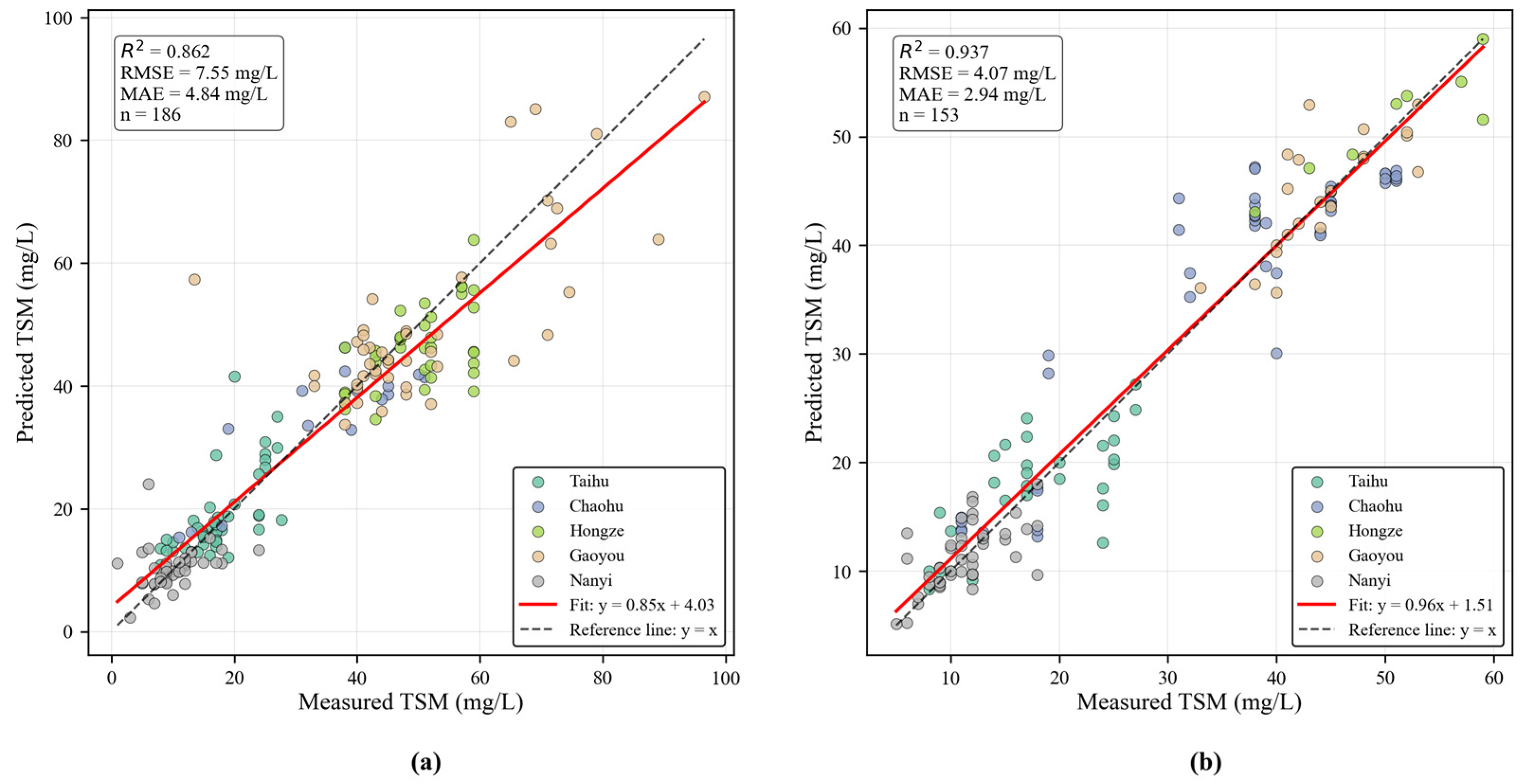
Figure 5 displays the scatter plots comparing predicted and measured TSM values from the final retrieval models based on GF-1 and Sentinel-2 imagery across the entire in situ dataset. The results indicated that the retrieval model constructed based on GF-1 images (Figure 5a) showed strong agreement with in situ measurements, with most scatter points closely clustered around the 1:1 line, resulting in an R² of 0.86. While scatter points from Taihu Lake, Chaohu Lake, and Nanyi Lake aligned more tightly along the 1:1 line, those from Gaoyou Lake and Hongze Lake tended to overestimate in some samples. In comparison, the retrieval model based on Sentinel-2 images demonstrated higher accuracy, with an R² exceeding 0.93. As shown in Figure 5b, the scatter points were consistently aligned along the 1:1 line, indicating a good fit for the measured data of all five lakes.

Figure 5. Performance evaluation of the derived TSM retrieval models on the in situ dataset: (a) Scatter plot of predicted versus measured TSM for the GF-1 derived model; (b) Scatter plot of predicted versus measured TSM for the Sentinel-2 derived model.

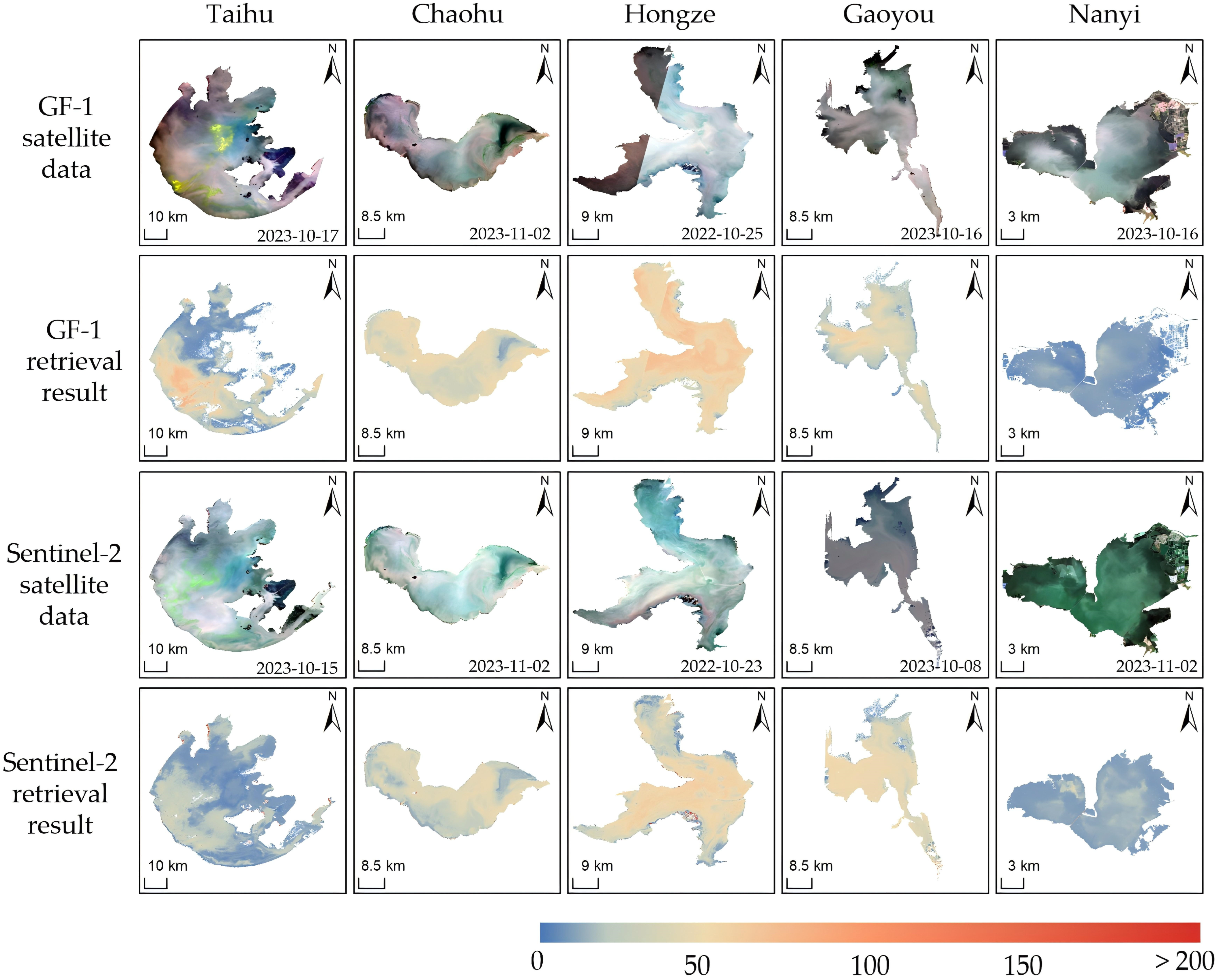
The spatial distribution of TSM in the five lakes are shown in Figure 6. The first and third rows of Figure 6 display the true-color composite images from GF-1 and Sentinel-2, respectively. Visual analysis revealed that the original imagery could, to some extent, reflect the TSM concentrations. Areas with low TSM concentrations appeared in turquoise, while regions with higher concentrations were characterized by brownish hues. The second and fourth rows of Figure 6 display the retrieval results based on GF-1 and Sentinel-2 imagery, respectively. Both retrieval results demonstrated a high spatial agreement with the TSM distributions in the original imagery and exhibited spatial aggregation patterns. In general, the TSM concentrations in Nanyi Lake were relatively low, with most areas having concentrations between 5 and 20 mg/L. In contrast, the TSM concentrations in Hongze Lake and Gaoyou Lake were higher, with both lakes exhibiting central high and peripheral low spatial distribution patterns. Specifically, TSM concentrations in most of Hongze Lake ranged from 40 to 70 mg/L, while those in Gaoyou Lake were primarily between 30 and 55 mg/L. The TSM concentration in Chaohu Lake displayed significant spatial heterogeneity, with the northeastern and southern areas having lower concentrations (mainly 5–35 mg/L), whereas the central lake area exhibited higher concentrations (40–60 mg/L). Taihu Lake followed a southwest-high, peripheral-low distribution pattern for TSM concentration. Notably, in the Taihu Lake region, the retrieval results based on GF-1 data showed higher concentration values and a more extensive high-concentration area. This discrepancy may be associated with the spatial reflectance patterns in the original imagery. Despite the imagery being acquired close in time (GF-1 on 17 October 2023, and Sentinel-2 on 15 October 2023), significant differences were observed in the Taihu Lake region. A distinct turquoise low-concentration area was visible in the center of the Sentinel-2 image, while this low-concentration region shifted northeastward and significantly shrank in the GF-1 image. This variation likely explains the differences observed in the retrieval results.

Figure 6. Spatial distribution of TSM retrieval results in five lakes based on GF-1 and Sentinel-2 imagery.

3.2. Validation and Comparison of TSM Retrieval Models

To evaluate the proposed DFE-SVR method, three representative approaches were selected for comparison in TSM retrieval from multispectral remote sensing data, namely BPNN, SVR, and the band-combination-based statistical regression algorithm (BCR). Specifically, the BPNN model was derived from the pre-training stage of the DFE-SVR model, while the SVR model was constructed using all available spectral bands. The BCR algorithm derived the optimal TSM retrieval model by selecting band combinations that exhibited strong correlations with TSM and establishing statistical regression relationships using various regression forms, such as linear and polynomial models. BCR was chosen as the benchmark owing to its simplicity and wide applicability.

Four TSM retrieval models (DFE-SVR, BPNN, SVR, and BCR) were developed using GF-1 imagery and validated on an independent test set. As shown in Table 2, the DFE-SVR model consistently outperformed the other approaches, achieving an MAE of 5.52, an RMSE of 7.95, and an R² of 0.85. The BCR model yielded the lowest accuracy with an MAE of 10.66, an RMSE of 14.07, and an R² of 0.54, suggesting that simple band combinations cannot adequately characterize the spectral response of TSM. The SVR model showed moderately good results, with an MAE of 7.74, an RMSE of 11.35, and an R² of 0.70. Meanwhile, the BPNN model showed improved accuracy, with an MAE of 5.60, an RMSE of 8.56, and an R² of 0.83. Nevertheless, both the SVR and BPNN models exhibited limited predictive ability compared to DFE-SVR.

Table 2. Accuracy of TSM retrieval models based on GF-1 imagery.

Method	Train Set			Test Set
	MAE	RMSE	R2	MAE	RMSE	R2
DFE-SVR	3.93	6.70	0.88	5.52	7.95	0.85
BCR	8.22	11.89	0.63	10.66	14.07	0.54
BPNN	4.94	7.22	0.86	5.60	8.56	0.83
SVR	7.65	10.64	0.71	7.74	11.35	0.70
PCA-SVR	7.67	10.78	0.70	8.16	11.69	0.68
BCT10-SVR	7.39	11.60	0.65	8.11	12.11	0.66

To further assess the feature extraction capability of DFE-SVR, two alternative feature representation strategies were tested. First, principal component analysis (PCA) was applied to the spectral bands to construct an SVR-based TSM model (PCA-SVR). Second, ten band combinations that are most strongly correlated with TSM were selected as input features for SVR modeling (BCT10-SVR). As shown in Table 2, both PCA-SVR and BCT10-SVR underperformed compared to the DFE-SVR, with R² values of 0.68 and 0.66, respectively, while DFE-SVR achieved an R² of 0.85. Notably, there was a slight reduction in accuracy for PCA-SVR and BCT10-SVR compared to SVR. This decline in accuracy is likely due to the loss of spectral information during PCA dimensionality reduction and feature selection in BCT10, as well as the limited representational capacity of manually selected band combinations.

The validation results based on Sentinel-2 imagery (Table 3) indicated that DFE-SVR again delivered the highest accuracy, with R² of 0.90. Both SVR and PCA-SVR performed well, with R² of 0.85, but were consistently outperformed by DFE-SVR and BPNN (R² = 0.87). The lowest accuracy was observed for the BCR model and BCT10-SVR, with R² of 0.83 and 0.80, respectively. For the BCR retrieval model based on GF-1 imagery, the BCR model for Sentinel-2 exhibited higher accuracy (R² = 0.54 vs. 0.83, RMSE = 14.07 vs. 6.41, MAE = 10.66 vs. 5.13). The accuracy of the Sentinel-2 BCR model was actually close to that of the BPNN or SVR-based models, suggesting a strong correlation between the spectral reflectance data from Sentinel-2 and TSM concentration, which enables the construction of relatively high-precision models directly from the spectral bands. In contrast, the spectral bands of GF-1 imagery exhibited a weak correlation with TSM concentration. By applying the method proposed in this study, the retrieval model showed significant improvement. For GF-1 imagery, the DFE-SVR model reduced MAE by 48.22% compared to the BCR model. For Sentinel-2 imagery, the DFE-SVR model reduced MAE by 33.53% compared to the BCR model. These results demonstrated that the method proposed in this study can effectively capture the complex spectral response to TSM concentration.

Table 3. Accuracy of TSM retrieval models based on Sentinel-2 imagery.

Method	Train Set			Test Set
	MAE	RMSE	R2	MAE	RMSE	R2
DFE-SVR	2.37	3.34	0.96	3.41	4.76	0.90
BCR	4.92	6.10	0.86	5.13	6.41	0.83
BPNN	2.51	3.23	0.96	4.68	5.55	0.87
SVR	3.70	5.13	0.90	5.02	6.05	0.85
PCA-SVR	3.79	5.23	0.90	4.83	5.92	0.85
BCT10-SVR	4.86	6.12	0.86	5.33	6.91	0.80

3.3. Effectiveness of the DFE-ML Framework Under Limited Samples

To evaluate the performance of the proposed DFE-SVR method when training samples are limited, experiments were conducted by training the models on 100%, 80%, 60%, 40%, and 20% of the original training set. The models were then tested on a unified, independent test set.

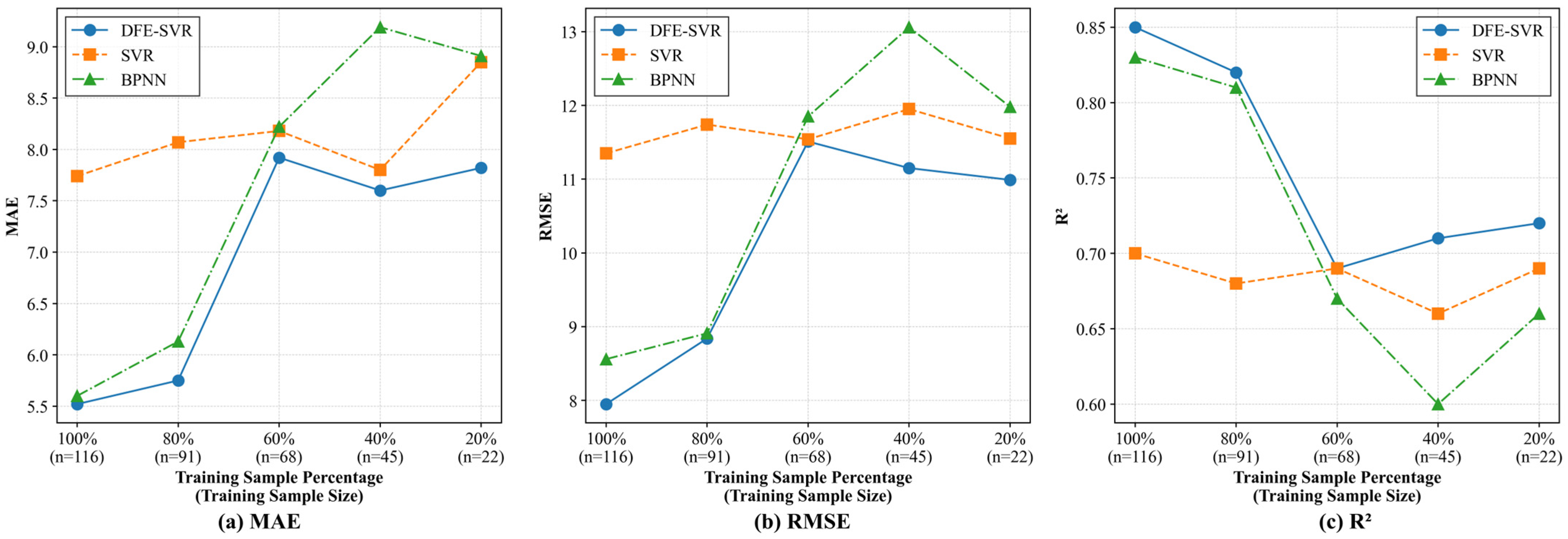
For GF-1 imagery, as the training sample ratio decreased from 100% to 20%, the R² of DFE-SVR dropped from 0.85 to 0.72, MAE increased from 5.52 to 7.82 and RMSE rose from 7.95 to 10.99 (Figure 7). In comparison, the SVR model exhibited relatively stable but poorer performance, with R² fluctuating between 0.66 and 0.70. The BPNN model experienced a more significant degradation, with its R² decreasing from 0.83 to 0.66. Notably, even with only 20% of the training samples, DFE-SVR achieved a higher R² (0.72) than both SVR (0.69) and BPNN (0.66). The smaller increases in MAE and RMSE for DFE-SVR compared to BPNN further validate its superior robustness under data-scarce conditions.

Figure 7. Performance comparison of the proposed method for TSM retrieval using GF-1 imagery under different training sample ratios, evaluated on an independent test set with 33 test samples: (a) MAE; (b) RMSE; (c) R².

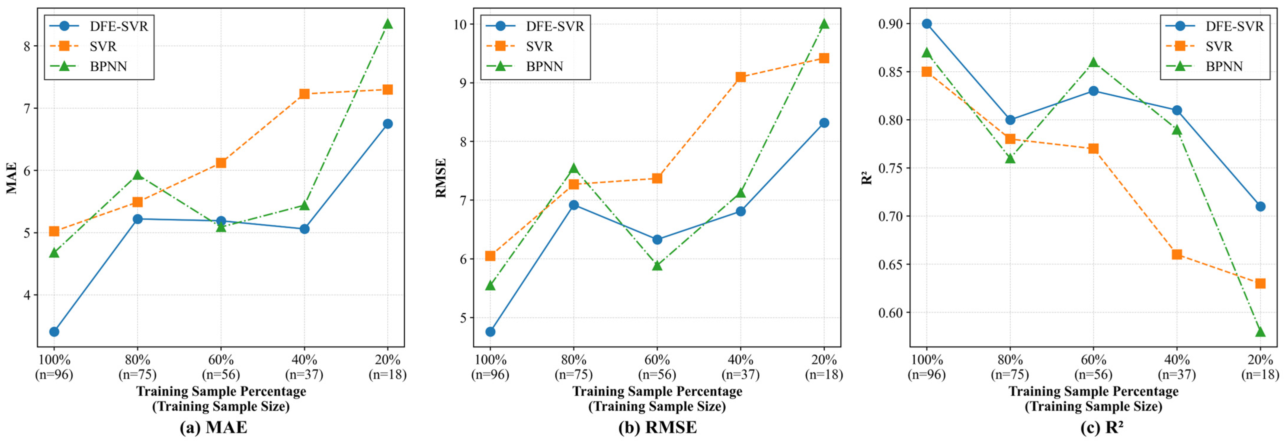
Similar trends were observed on the Sentinel-2 imagery (Figure 8). For DFE-SVR, R² declined from 0.90 to 0.71 as the training sample percentage decreased, with MAE rising from 3.41 to 6.75 and RMSE from 4.76 to 8.32. The comparative models exhibited a more significant performance deterioration, with R² of the SVR model decreasing from 0.85 to 0.63 and R² of the BPNN model dropping from 0.87 to 0.58. When trained with merely 20% of the samples, DFE-SVR (R² = 0.71) significantly outperformed both SVR (R² = 0.63) and BPNN (R² = 0.58). The smaller increases in MAE and RMSE for DFE-SVR demonstrate its consistent superiority across diverse remote sensing data sources, especially under conditions of limited sample availability.

Figure 8. Performance comparison of the proposed method for TSM retrieval using Sentinel-2 imagery under different training ratios, evaluated on an independent test set with 26 test samples: (a) MAE; (b) RMSE; (c) R².

4. Discussion

4.1. Applicability of the DFE-ML Framework to Other Machine Learning Algorithms

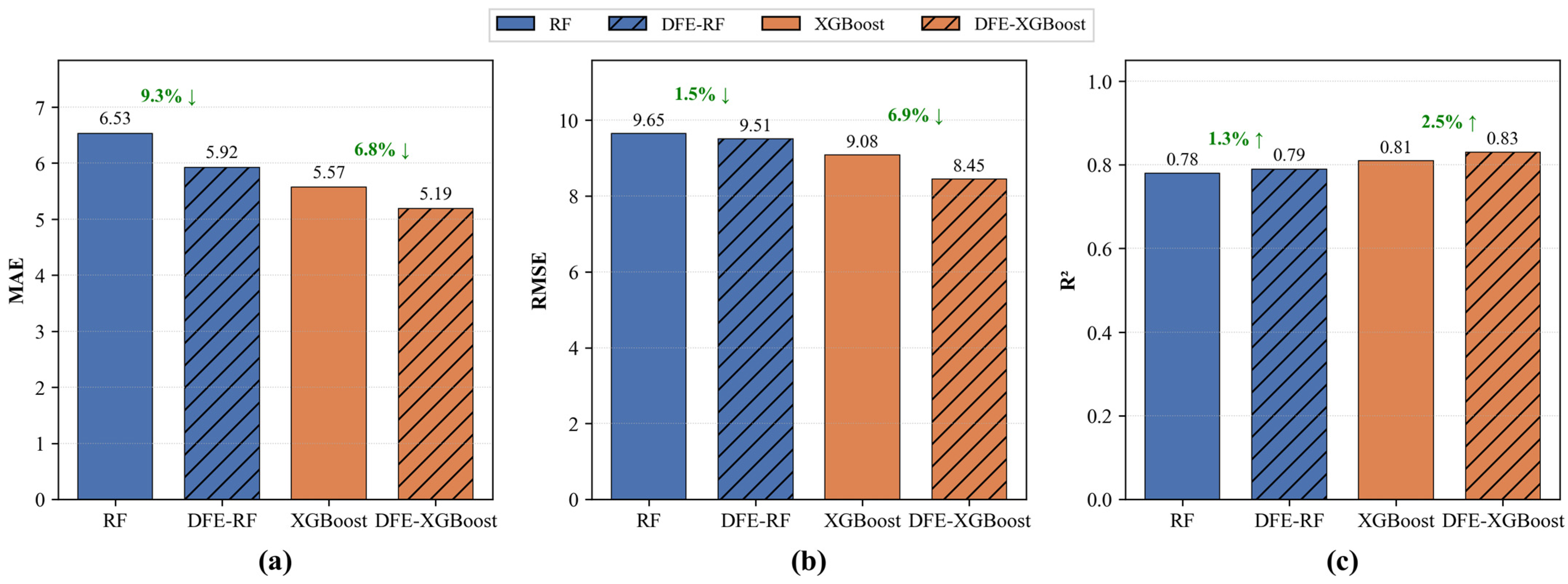
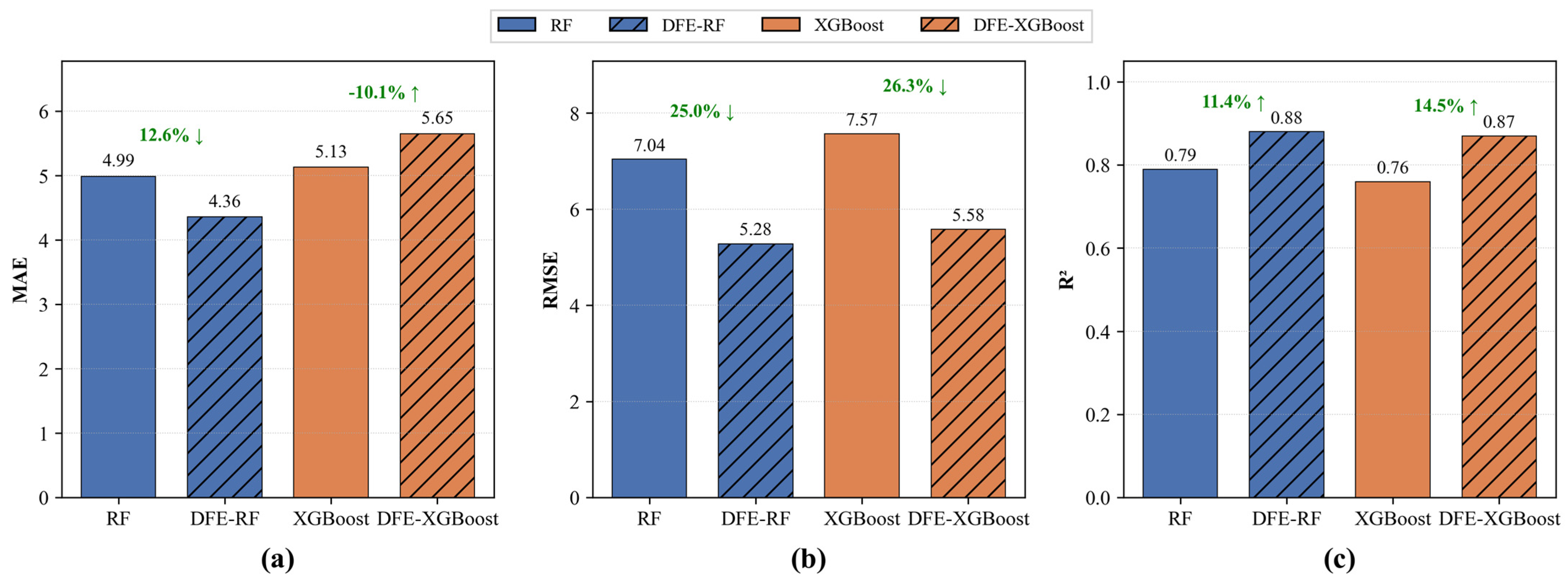
Furthermore, to evaluate the adaptability of the proposed framework, the DFE-ML framework was applied to two widely used algorithms for water quality parameter retrieval, RF and extreme gradient boosting (XGBoost), resulting in the DFE-RF and DFE-XGBoost models. The performance of these models was compared with their baseline counterparts (RF, XGBoost), with the results shown in Figure 9 and Figure 10. Overall, the models incorporating the DFE-ML framework demonstrated superior performance across all accuracy metrics.

Figure 9. Accuracy of the DFE-ML framework with other machine learning algorithms for TSM retrieval using GF-1 imagery: (a) MAE; (b) RMSE; (c) R².

Figure 10. Accuracy of the DFE-ML framework with other machine learning algorithms for TSM retrieval using Sentinel-2 imagery: (a) MAE; (b) RMSE; (c) R².

For GF-1 imagery (Figure 9), compared to the original models, DFE-RF and DFE-XGBoost reduced MAE by 9.3% and 6.8%, and RMSE by 1.5% and 6.9%, respectively. The R² of DFE-RF improved from 0.78 to 0.79, while DFE-XGBoost’s R² increased from 0.81 to 0.83. Similar trends were observed for Sentinel-2 imagery (Figure 10). For RF, the DFE-RF model improved from MAE = 4.99, RMSE = 7.04 and R² = 0.79 to MAE = 4.36, RMSE = 5.28 and R² = 0.88. For XGBoost, the performance gains were less pronounced but still evident. The DFE-XGBoost model achieved a lower RMSE (5.58 vs. 7.57) and a higher R² (0.87 vs. 0.76); despite a slight increase in MAE (5.65 vs. 5.13), resulting in an overall improvement in predictive accuracy.

4.2. Advantages

This study presents a practical and efficient TSM retrieval modeling framework for multispectral remote sensing imagery. Validation results showed that this framework substantially improves the retrieval stability with limited samples (Figure 7 and Figure 8). As the training sample ratio decreased from 100% to 20%, the DFE-SVR model exhibited a smaller decline in accuracy and slower increases in MAE and RMSE compared to the conventional SVR and BPNN models for both GF-1 and Sentinel-2 imagery. Even with only 20% of the training data, DFE-SVR maintained a higher R² and lower error metrics than the other models, highlighting its robustness to sample scarcity and its superior generalization capability. This consistent trend across both sensors suggests that the DFE-SVR framework is not overly dependent on specific spectral configurations but effectively captures the fundamental relationships between multispectral reflectance and TSM. The smaller degradation observed in DFE-SVR performance can be attributed to its two-stage design, which combines the nonlinear representation capability of deep neural networks with the stability of statistical regression. In this configuration, a BPNN first extracts high-level spectral features that capture complex nonlinear interactions, while the SVR regressor built upon these features mitigates overfitting, which is a common issue when training deep networks with limited samples. The resulting hybrid strategy provides an implicit form of regularization, allowing the model to generalize better from fewer observations. The similar behavior observed between GF-1 and Sentinel-2 further confirms the cross-sensor robustness of this approach, as their distinct spectral and spatial resolutions still yield consistent trends in accuracy and error metrics. This indicates that the framework leverages transferable relationships between spectral features and TSM, which are less sensitive to sensor-specific characteristics.

Furthermore, the deep feature extraction module within the DFE-ML framework enhances the ability to capture nonlinear spectral information. Compared to the BCR, full-band SVR, and PCA-SVR methods, DFE-SVR more effectively models the complex nonlinear relationship between multispectral data and TSM. Experiments conducted on both GF-1 and Sentinel-2 imagery consistently showed that DFE-SVR achieved better fitting performance and lower prediction errors in both training and test sets (Table 2 and Table 3). These results suggested that the deep features provide a more discriminative representation, enabling the model to overcome the limitations of traditional statistical regression and manual feature selection, thereby significantly improving retrieval accuracy. The effectiveness of the deep feature extraction strategy was further validated by applying the framework to other machine learning methods, such as RF and XGBoost. This confirms that the DFE-ML framework is not only an improvement for SVR, but also serves as a general-purpose preprocessing tool that can be integrated into various modeling frameworks, demonstrating its potential for broader application in aquatic remote sensing.

4.3. Limitations

Despite the promising performance of the DFE-ML framework, several limitations should be considered.

First, while the framework exhibited robustness with limited samples, training the deep feature extractor may become unstable with extremely limited data. Future research could explore integrating semi-supervised or transfer learning strategies to use unlabeled data, thereby enhancing generalization capabilities in such data-scarce scenarios. In addition, this study did not perform a full uncertainty quantification regarding sampling variability and instrument measurement error. Repeated measurements at fixed stations and inter-laboratory comparisons would help refine model accuracy and reliability. Future studies should also incorporate uncertainty and sensitivity analyses, such as evaluating the effects of temporal mismatch between field sampling and satellite overpasses or the impact of atmospheric correction accuracy, to better understand error propagation and improve model robustness and interpretability. Furthermore, cloud computing technologies could be considered in future work to enable large-scale and high-frequency monitoring of TSM.

Second, regarding model structure and comparison, the benchmark models were intentionally selected to address the challenge of limited samples. While end-to-end deep learning architectures (e.g., CNNs and LSTMs) are powerful under data-rich conditions, they were not included here because their large parameter space makes them prone to overfitting on small datasets, leading to an unfair and uninformative comparison. Evaluating the DFE-ML framework against such deep architectures on larger datasets remains a valuable direction for future work. Moreover, the physical meaning of the extracted deep features has not been thoroughly examined. Further investigation into the relationship between the learned representations and TSM-sensitive spectral bands would help provide a more theoretical understanding of the framework’s underlying mechanisms.

Third, although this study validated the framework using GF-1 and Sentinel-2 imagery, its applicability to other multispectral or hyperspectral sensors warrants further investigation. The DFE-ML framework is designed to be generically applicable to reflectance data from any sensor possessing key bands in the visible and near-infrared regions. Future work will validate and adapt this approach for other satellite systems, such as Landsat and MODIS, and explore its potential for hyperspectral applications. Extending the framework to non-optically active water quality parameters, such as nitrogen and phosphorus, will also help demonstrate its broader utility beyond optically active constituents.

5. Conclusions

This study developed a DFE-ML framework for regional TSM retrieval from multispectral remote sensing imagery, particularly designed to address the challenge of limited in situ samples. By combining the deep feature representation capability of a pre-trained BPNN with the robustness of SVR, the DFE-SVR model effectively captured the nonlinear relationships between spectral reflectance and TSM concentration. Validation experiments using in situ data from five inland lakes in Jiangsu and Anhui Provinces, China (Taihu, Gaoyou, Chaohu, Hongze, and Nanyi), demonstrated that the DFE-SVR model consistently outperformed conventional SVR and BPNN methods on both GF-1 and Sentinel-2 imagery, especially when the availability of in situ data was limited. The model achieved higher R² and lower RMSE than traditional approaches, maintaining strong stability and generalization even when the training samples were reduced to 20%. The DFE-ML framework also improved the discriminative power of spectral features, overcoming the limitations of manual feature selection and traditional statistical regression methods. Moreover, the framework was successfully extended to other machine learning algorithms, including RF and XGBoost, confirming its potential as a general preprocessing and modeling strategy for multispectral water-quality retrieval.

Above all, the proposed method significantly reduces the dependency on large in situ datasets for high-quality TSM retrieval, establishing a viable pathway for low-cost, high-frequency water quality monitoring. This capability will empower relevant authorities to track water quality dynamics promptly, assess ecological health, and provide sustained data support for optimizing and evaluating watershed management policies.

Future work will focus on extending the DFE-ML framework to other water quality parameters and incorporating uncertainty analysis. The exploration of semi-supervised or transfer learning strategies will also be pursued to enhance performance under extremely limited in situ measurements.

References

1. Giri, S. Water Quality Prospective in Twenty First Century: Status of Water Quality in Major River Basins, Contemporary Strategies and Impediments: A Review. Environ. Pollut. 2021, 271, 116332. [Google Scholar] [CrossRef] [PubMed]
2. Zhang, Y.; Wu, L.; Deng, L.; Ouyang, B. Retrieval of Water Quality Parameters from Hyperspectral Images Using a Hybrid Feedback Deep Factorization Machine Model. Water Res. 2021, 204, 117618. [Google Scholar] [CrossRef] [PubMed]
3. Yin, Z.; Li, J.; Liu, Y.; Zhang, F.; Wang, S.; Xie, Y.; Gao, M. Decline of Suspended Particulate Matter Concentrations in Lake Taihu from 1984 to 2020: Observations from Landsat TM and OLI. Opt. Express 2022, 30, 22572–22589. [Google Scholar] [CrossRef]
4. Feng, L.; Hu, C.; Chen, X.; Song, Q. Influence of the Three Gorges Dam on Total Suspended Matters in the Yangtze Estuary and Its Adjacent Coastal Waters: Observations from MODIS. Remote Sens. Environ. 2014, 140, 779–788. [Google Scholar] [CrossRef]
5. Wang, J.; Sun, D.; Wang, S.; Li, Z.; Zhang, Y.; Li, J.; Zhang, H. Satellite Observations of Suspended Particulate Matter Concentration in Lake Gaoyou in the Past Four Decades. Water Res. 2024, 254, 121442. [Google Scholar] [CrossRef] [PubMed]
6. Blix, K.; Pálffy, K.; Tóth, V.R.; Eltoft, T. Remote Sensing of Water Quality Parameters over Lake Balaton by Using Sentinel-3 OLCI. Water 2018, 10, 1428. [Google Scholar] [CrossRef]
7. Cui, J.S.; Lv, P.Y. Turbidity Effect on the Fluorescence Determination of Chlorophyll-a in Water. Appl. Mech. Mater. 2014, 522, 60–63. [Google Scholar] [CrossRef]
8. Zhao, J.; Cao, W.; Xu, Z.; Ye, H.; Yang, Y.; Wang, G.; Zhou, W.; Sun, Z. Estimation of Suspended Particulate Matter in Turbid Coastal Waters: Application to Hyperspectral Satellite Imagery. Opt. Express 2018, 26, 10476–10493. [Google Scholar] [CrossRef]
9. Swift, T.J.; Perez-Losada, J.; Schladow, S.G.; Reuter, J.E.; Jassby, A.D.; Goldman, C.R. Water Clarity Modeling in Lake Tahoe: Linking Suspended Matter Characteristics to Secchi Depth. Aquat. Sci. 2006, 68, 1–15. [Google Scholar] [CrossRef]
10. Binding, C.E.; Bowers, D.G.; Mitchelson-Jacob, E.G. Estimating Suspended Sediment Concentrations from Ocean Colour Measurements in Moderately Turbid Waters; the Impact of Variable Particle Scattering Properties. Remote Sens. Environ. 2005, 94, 373–383. [Google Scholar] [CrossRef]
11. V.-Balogh, K.; Németh, B.; Vörös, L. Specific Attenuation Coefficients of Optically Active Substances and Their Contribution to the Underwater Ultraviolet and Visible Light Climate in Shallow Lakes and Ponds. Hydrobiologia 2009, 632, 91–105. [Google Scholar] [CrossRef]
12. Liu, X.; Zhang, Z.; Jiang, T.; Li, X.; Li, Y. Evaluation of the Effectiveness of Multiple Machine Learning Methods in Remote Sensing Quantitative Retrieval of Suspended Matter Concentrations: A Case Study of Nansi Lake in North China. J. Spectrosc. 2021, 2021, 5957376. [Google Scholar] [CrossRef]
13. Adjovu, G.E.; Stephen, H.; James, D.; Ahmad, S. Measurement of Total Dissolved Solids and Total Suspended Solids in Water Systems: A Review of the Issues, Conventional, and Remote Sensing Techniques. Remote Sens. 2023, 15, 3534. [Google Scholar] [CrossRef]
14. Wang, C.; Li, W.; Chen, S.; Li, D.; Wang, D.; Liu, J. The Spatial and Temporal Variation of Total Suspended Solid Concentration in Pearl River Estuary during 1987–2015 Based on Remote Sensing. Sci. Total Environ. 2018, 618, 1125–1138. [Google Scholar] [CrossRef]
15. Yang, H.; Kong, J.; Hu, H.; Du, Y.; Gao, M.; Chen, F. A Review of Remote Sensing for Water Quality Retrieval: Progress and Challenges. Remote Sens. 2022, 14, 1770. [Google Scholar] [CrossRef]
16. Bubnova, E.; Bukanova, T.; Kopelevich, O.; Vazyulya, S.; Sahling, I. Spatial-Temporal Variations of the Total Suspended Matter Concentration in the South-Eastern Baltic. In Proceedings of the 2018 IEEE/OES Baltic International Symposium (BALTIC), Klaipeda, Lithuania, 12–15 June 2018; pp. 1–9. [Google Scholar]
17. Friedmann, E.; Gleason, C.J.; Feng, D.; Langhorst, T. Estimating Riverine Total Suspended Solids from Spatiotemporal Satellite Sensor Fusion. IEEE J. Sel. Top. Appl. Earth Obs. Remote Sens. 2024, 17, 15443–15462. [Google Scholar] [CrossRef]
18. Lei, S.; Xu, J.; Li, Y.; Du, C.; Liu, G.; Zheng, Z.; Xu, Y.; Lyu, H.; Mu, M.; Miao, S.; et al. An Approach for Retrieval of Horizontal and Vertical Distribution of Total Suspended Matter Concentration from GOCI Data over Lake Hongze. Sci. Total Environ. 2020, 700, 134524. [Google Scholar] [CrossRef]
19. Hou, X.; Feng, L.; Duan, H.; Chen, X.; Sun, D.; Shi, K. Fifteen-Year Monitoring of the Turbidity Dynamics in Large Lakes and Reservoirs in the Middle and Lower Basin of the Yangtze River, China. Remote Sens. Environ. 2017, 190, 107–121. [Google Scholar] [CrossRef]
20. Alcântara, E.; Curtarelli, M.; Ogashawara, I.; Rosan, T.; Kampel, M.; Stech, J. Developing QAA-Based Retrieval Model of Total Suspended Matter Concentration in Itumbiara Reservoir, Brazil. In Proceedings of the 2015 IEEE International Geoscience and Remote Sensing Symposium (IGARSS), Milan, Italy, 26–31 July 2015; pp. 711–714. [Google Scholar]
21. Chen, J.; Cui, T.; Qiu, Z.; Lin, C. A Three-Band Semi-Analytical Model for Deriving Total Suspended Sediment Concentration from HJ-1A/CCD Data in Turbid Coastal Waters. ISPRS J. Photogramm. Remote Sens. 2014, 93, 1–13. [Google Scholar] [CrossRef]
22. Lee, Z.; Weidemann, A.; Kindle, J.; Arnone, R.; Carder, K.L.; Davis, C. Euphotic Zone Depth: Its Derivation and Implication to Ocean-Color Remote Sensing. J. Geophys. Res. Ocean. 2007, 112, C03009. [Google Scholar] [CrossRef]
23. Xie, Y.; Zhou, Y.; Tao, Z.; Shao, W.; Yang, M. Remote Sensing Inversion of the Total Suspended Matter Concentration in the Nanyi Lake Based on Sentinel-3 OLCI Imagery. IEEE J. Sel. Top. Appl. Earth Obs. Remote Sens. 2024, 17, 10380–10389. [Google Scholar] [CrossRef]
24. Zhu, P.; Liu, Y.; Li, J. Optimization and Evaluation of Widely-Used Total Suspended Matter Concentration Retrieval Methods for ZY1-02D’s AHSI Imagery. Remote Sens. 2022, 14, 684. [Google Scholar] [CrossRef]
25. Chen, S.; Jiang, L.; Cheng, X.; Liao, G.; Gerkema, T. A Physical Perspective of Recurrent Water Quality Degradation: A Case Study in the Jiangsu Coastal Waters, China. J. Geophys. Res. Ocean. 2023, 128, e2022JC019607. [Google Scholar] [CrossRef]
26. Sims, D.A.; Gamon, J.A. Relationships between Leaf Pigment Content and Spectral Reflectance across a Wide Range of Species, Leaf Structures and Developmental Stages. Remote Sens. Environ. 2002, 81, 337–354. [Google Scholar] [CrossRef]
27. Forget, P.; Ouillon, S.; Lahet, F.; Broche, P. Inversion of Reflectance Spectra of Nonchlorophyllous Turbid Coastal Waters. Remote Sens. Environ. 1999, 68, 264–272. [Google Scholar] [CrossRef]
28. Cui, J.; Cao, X.; Du, C.; Dong, W.; Liu, S.; Guo, J.; Xu, M.; Yasir, M. Chl-a Concentration Inversion Methods for Water Bodies With High TSM Concentrations Based on Waterbody Classification and Deep Learning. IEEE J. Sel. Top. Appl. Earth Obs. Remote Sens. 2025, 18, 5673–5686. [Google Scholar] [CrossRef]
29. Jalagam, L.; Shepherd, N.; Qi, J.; Barclay, N.; Smith, M. Water Quality Predictions for Urban Streams Using Machine Learning. In Proceedings of the SoutheastCon 2023, Orlando, FL, USA, 14–16 April 2023; pp. 217–223. [Google Scholar]
30. Alpizar, L.H.; Mejía, J.A.G. Modeling Surface Water Quality Using K-Nearest Neighbors and Random Forest. In Proceedings of the 2024 IEEE 6th International Conference on BioInspired Processing (BIP), Liberia, Costa Rica, 4–6 December 2024; pp. 1–5. [Google Scholar]
31. Guo, H.; Tian, S.; Huang, J.J.; Zhu, X.; Wang, B.; Zhang, Z. Performance of Deep Learning in Mapping Water Quality of Lake Simcoe with Long-Term Landsat Archive. ISPRS J. Photogramm. Remote Sens. 2022, 183, 451–469. [Google Scholar] [CrossRef]
32. Fang, X.; Wen, Z.; Chen, J.; Wu, S.; Huang, Y.; Ma, M. Remote Sensing Estimation of Suspended Sediment Concentration Based on Random Forest Regression Model. Natl. Remote Sens. Bull. 2019, 23, 756–772. [Google Scholar] [CrossRef]
33. Kupssinskü, L.S.; Guimarães, T.T.; de Freitas, R.; de Souza, E.M.; Rossa, P.; Marques, A.; Veronez, M.R.; Gonzaga, L.; Cazarin, C.L.; Mauad, F.F. Prediction of Chlorophyll-a and Suspended Solids through Remote Sensing and Artificial Neural Networks. In Proceedings of the 2019 13th International Conference on Sensing Technology (ICST), Sydney, NSW, Australia, 2–4 December 2019; pp. 1–6. [Google Scholar]
34. Huang, P.; Huang, Y. Spatial-Temporal Patterns of Total Suspended Matters (TSM) in the Yellow River Estuary. In Proceedings of the IGARSS 2020—2020 IEEE International Geoscience and Remote Sensing Symposium, Waikoloa, HI, USA, 26 September–2 October 2020; pp. 5773–5776. [Google Scholar]
35. Zhang, M.; Tang, J.; Dong, Q.; Song, Q.; Ding, J. Retrieval of Total Suspended Matter Concentration in the Yellow and East China Seas from MODIS Imagery. Remote Sens. Environ. 2010, 114, 392–403. [Google Scholar] [CrossRef]
36. Xia, X.; Lu, H.; Xu, Z.; Li, X.; Tian, Y. Research on the Characteristic Spectral Band Determination for Water Quality Parameters Retrieval Based on Satellite Hyperspectral Data. Remote Sens. 2023, 15, 5578. [Google Scholar] [CrossRef]
37. Kwon, S.; Shin, J.; Seo, I.W.; Noh, H.; Jung, S.H.; You, H. Measurement of Suspended Sediment Concentration in Open Channel Flows Based on Hyperspectral Imagery from UAVs. Adv. Water Resour. 2022, 159, 104076. [Google Scholar] [CrossRef]
38. Yasir, M.; Shanwei, L.; Mingming, X.; Jianhua, W.; Hui, S.; Nazir, S.; Zhang, X.; Colak, A.T.I. YOLOv8-BYTE: Ship Tracking Algorithm Using Short-Time Sequence SAR Images for Disaster Response Leveraging GeoAI. Int. J. Appl. Earth Obs. Geoinf. 2024, 128, 103771. [Google Scholar] [CrossRef]
39. Zhang, J.; Li, H.; Miao, Y.; Zhou, Z.; Lyu, H.; Gong, Z. Remote Sensing Retrieval Method Based on Few-Shot Learning: A Case Study of Surface Dissolved Organic Carbon in Jiangsu Coastal Waters, China. IEEE Access 2025, 13, 3014–3025. [Google Scholar] [CrossRef]
40. Jalil, A.; Li, Y.; Zhang, K.; Gao, X.; Wang, W.; Khan, H.O.S.; Pan, B.; Ali, S.; Acharya, K. Wind-Induced Hy-drodynamic Changes Impact on Sediment Resuspension for Large, Shallow Lake Taihu, China. Int. J. Sediment Res. 2019, 34, 205–215. [Google Scholar] [CrossRef]
41. Liu, B.; Cai, S.; Wang, H.; Cui, C.; Cao, X. Hydrodynamics and Water Quality of the Hongze Lake in Response to Human Activities. Environ. Sci. Pollut. Res. 2021, 28, 46215–46232. [Google Scholar] [CrossRef]
42. Li, S.; Guo, W.; Yin, Y.; Jin, X.; Tang, W. Environmental Changes Inferred from Lacustrine Sediments and Historical Literature: A Record from Gaoyou Lake, Eastern China. Quat. Int. 2015, 380–381, 350–357. [Google Scholar] [CrossRef]
43. Luo, W.; Fan, Y.; Lu, J.; Zhu, S. Nutrient Distribution and Interrelationships in Chaohu Lake, China: Insights from Sedimentary Records. Expo. Health 2025, 17, 863–873. [Google Scholar] [CrossRef]
44. Li, G.; Li, X.; Jiang, X.; Zhang, Y.; Li, H.; Zhang, J.; Cai, G.; Luo, K.; Xie, F. Occurrence and Source Analysis of Heavy Metals and Dissolved Organic Matter in Nanyi Lake, Anhui Province. Environ. Monit. Assess. 2023, 195, 660. [Google Scholar] [CrossRef]
45. Loisel, H.; Mangin, A.; Vantrepotte, V.; Dessailly, D.; Dinh, D.N.; Garnesson, P.; Ouillon, S.; Lefebvre, J.-P.; Mériaux, X.; Phan, T.M. Variability of Suspended Particulate Matter Concentration in Coastal Waters under the Mekong’s Influence from Ocean Color (MERIS) Remote Sensing over the Last Decade. Remote Sens. Environ. 2014, 150, 218–230. [Google Scholar] [CrossRef]
46. Teng, W.; Yu, Q.; Stramski, D.; Reynolds, R.A.; Woodruff, J.D.; Yellen, B. High Spatial-Resolution Satellite Mapping of Suspended Particulate Matter in Global Coastal Waters Using Particle Composition-Adaptive Algorithms. Remote Sens. Environ. 2025, 323, 114745. [Google Scholar] [CrossRef]
47. Chen, Z.; Dou, M.; Xia, R.; Li, G.; Shen, L. Spatiotemporal Evolution of Chlorophyll-a Concentration from MODIS Data Inversion in the Middle and Lower Reaches of the Hanjiang River, China. Environ. Sci. Pollut. Res. 2022, 29, 38143–38160. [Google Scholar] [CrossRef] [PubMed]
48. Park, Y.; Cho, K.H.; Park, J.; Cha, S.M.; Kim, J.H. Development of Early-Warning Protocol for Predicting Chlorophyll-a Concentration Using Machine Learning Models in Freshwater and Estuarine Reservoirs, Korea. Sci. Total Environ. 2015, 502, 31–41. [Google Scholar] [CrossRef] [PubMed]
49. Zhou, S. An Analysis of The Small Sample Datasets Based on Machine Learning. In Proceedings of the 2022 6th International Conference on Electronic Information Technology and Computer Engineering, Xiamen, China, 21–23 October 2022; Association for Computing Machinery: New York, NY, USA, 2023; pp. 1654–1658. [Google Scholar]
50. Seegers, B.N.; Stumpf, R.P.; Schaeffer, B.A.; Loftin, K.A.; Werdell, P.J. Performance Metrics for the Assessment of Satellite Data Products: An Ocean Color Case Study. Opt. Express 2018, 26, 7404–7422. [Google Scholar] [CrossRef] [PubMed]
51. Peterson, K.T.; Sagan, V.; Sidike, P.; Cox, A.L.; Martinez, M. Suspended Sediment Concentration Estimation from Landsat Imagery along the Lower Missouri and Middle Mississippi Rivers Using an Extreme Learning Machine. Remote Sens. 2018, 10, 1503. [Google Scholar] [CrossRef]
52. Larson, M.D.; Milas, A.S.; Vincent, R.K.; Evans, J.E. Landsat 8 Monitoring of Multi-Depth Suspended Sediment Concentrations in Lake Erie’s Maumee River Using Machine Learning. Int. J. Remote Sens. 2021, 42, 4064–4086. [Google Scholar] [CrossRef]
Disclaimer/Publisher’s Note: The statements, opinions and data contained in all publications are solely those of the individual author(s) and contributor(s) and not of MDPI and/or the editor(s). MDPI and/or the editor(s) disclaim responsibility for any injury to people or property resulting from any ideas, methods, instructions or products referred to in the content.
Article Metrics
Citations
Article Access Statistics
Multiple requests from the same IP address are counted as one view.