Groundwater Level Response to Precipitation and Potential Climate Trends

Abstract

Stream–aquifer interactions, as well as surface water/groundwater interactions within wetlands, require a solution of complex partial differential equations of flow and contaminant transport, namely a deterministic approach. Groundwater level (GWL) responses to precipitation, particularly for extreme value events such as annual maxima, require a probabilistic approach to evaluate potential climate trends. It is commonly assumed that the distribution of annual maxima series (AMS) precipitation follows the generalized extreme value distribution (GEV). If the extremes of the data are nonstationary, it is possible to incorporate this knowledge into the parameters of the GEV. This approach is also applied to the computed annual maxima of daily groundwater level data. Nonstationary versus stationary time series for both groundwater level and AMS 24-h duration precipitation are compared for National Oceanic and Atmospheric Administration (NOAA) stations with nearby wells. Predicted extreme value analysis (EVA) climate trends for wells penetrating limestone aquifers directly beneath rainfall monitoring stations at major airports indicate similar GWL response. Groundwater levels at wells located near coastlines are partially impacted by sea level rise. An extreme value analysis of the GWL is shown to be a useful tool to confirm hydrologic connections and long-term climate trends.

1. Introduction

Stream–aquifer interactions, as well as surface water/groundwater interactions within wetlands, require a solution of complex partial differential equations of flow and contaminant transport, namely a deterministic approach, for example, the incorporation of transient storage in a conjunctive stream–aquifer modeling application [1]. The physical/chemical processes and interactions involved in such a conjunctive stream–aquifer simulation can be illustrated in Figure 1 and Figure 2. Similarly, a wetland hydrology and water quality model incorporating surface water/groundwater interactions was applied to a constructed wetland located within the Duke University campus [2]. The model accounted for upstream contributions from urbanized areas. The effect of restored wetlands on storm water runoff was also investigated by routing the overland flow through the wetland area, collecting the runoff within the stream, and transporting it to the receiving water using diffusion wave routing techniques. The components of the WETSAND model are illustrated in Figure 3. These deterministic modeling approaches would be impractical for the evaluation of groundwater level responses to long precipitation time series of extreme value events (such as annual maxima) to subsequently predict potential climate trends. A probabilistic approach is required.

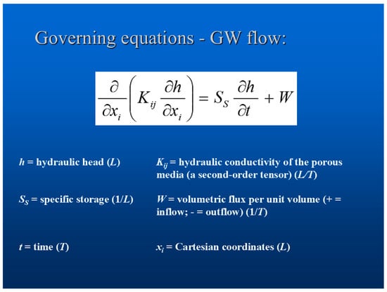
Figure 1. Deterministic groundwater flow [1].

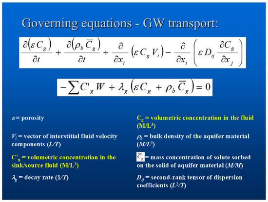
Figure 2. Deterministic groundwater transport [1].

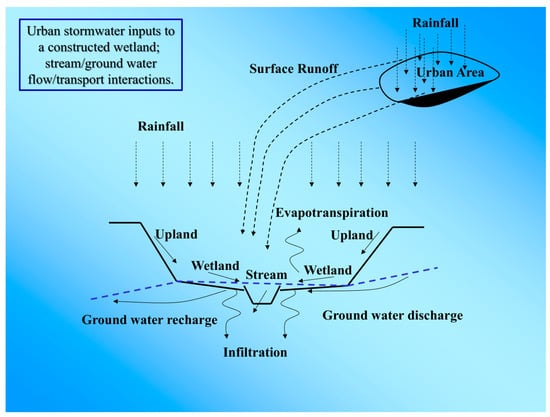
Figure 3. Hydrological components of the WETSAND model [2].

The definition of extreme events is, in general terms, that they constitute relatively rare events with a low probability of recurring at specific locations; nevertheless, these events (e.g., record rainfall, peak streamflow, sea level rise) can produce severe impacts on the infrastructure. More recently, it has been suggested that shallow emerging coastal groundwater is a hazard that is at least broadly comparable in terms of socioeconomic exposure to surface flooding [3]. As part of the water and climate resilience metrics, the South Florida Water Management District (SFWMD) has included groundwater levels in South Florida in the metrics required to track [4]. Assuming stationarity in the rainfall or groundwater level record may indeed miss climate change trends (for either increasing or decreasing values). Some hydrologists argue that hydrologic processes have never been stationary and will never be, since hydrologic observations typically consist of both deterministic and stochastic components [5]. Other studies of climate change impact on groundwater levels applied extreme value statistics on predictions from global climate models and regional hydrological models using the Gumbel approach [6,7].

2. Materials and Methods

2.1. Nonstationary Methods for Analyzing Extreme Events

If it is believed that the extremes of the data are nonstationary, then it is possible to incorporate this knowledge into the parameters. For example, we can assume that the location parameter of the extreme probability distribution selected is a linear function of time (of log-transformed values):

$${\mu }_t={\mu }_0+{\mu }_1 t$$

(1)

where µ₀ = signifies the intercept (usually the mean value of the distribution for the first year of the record) and µ₁ = the slope of the linear function, while keeping the scale (σ) and shape (Ɛ) parameters constant. The location parameter represents the most likely value of the distribution chosen. The values of µ_t must then be transformed back from log-transformed values. The use of a constant value for σ means that the standard deviation of the arithmetic record peaks will increase with the logarithmic mean distribution. This property is desirable since nonstationarity would likely not only alter the mean of the peaks but also affect their associated dispersion. For example, a trend in the scale parameter is as follows:

$$\ln {\sigma }_t={\sigma }_0+bt$$

(2)

where σ₀ and b are constants. It is commonly assumed that the distribution of annual maxima series (AMS) precipitation follows the generalized extreme value distribution (GEV) [5,7]:

$$\begin{array}{l}f\left(x | \mu ,\sigma ,\xi \right)={\displaystyle \frac{1}{\sigma }}{\left[1+\xi {\displaystyle \frac{\left(x-\mu \right)}{\sigma }}\right]}^{-1-1/\xi }exp\left\{-{\left[1+\xi {\displaystyle \frac{\left(x-\mu \right)}{\sigma }}\right]}^{-1/\xi }\right\}\\ where 1+\xi {\displaystyle \frac{\left(x-\mu \right)}{\sigma }}>0 and \sigma >0\end{array}$$

(3)

X = annual maximum precipitation; µ = location parameter;

σ = the scale parameter (>0); and ξ = the shape parameter.

The location parameter (µ) describes the center of the distribution; the scale parameter (σ) describes the distribution of the data around µ; and the shape parameter (ξ) defines the tail behavior of the distribution. If the shape parameter (ξ) is zero, the Gumbel distribution is used:

$$f(x | \mu ,\sigma ) = {\displaystyle \frac{1}{\sigma }}\exp \left(-{\displaystyle \frac{x-\mu }{\sigma }}\right)\exp \left[-\exp \left(-{\displaystyle \frac{x-\mu }{\sigma }}\right)\right]$$

(4)

Software is available to perform a GEV nonstationary extreme value analysis, for example, Matlab code NEVA [8] and the freely available extRemes R package [9,10]. The quantiles of the GEV may be interpreted as return levels, the value expected to be exceeded on average once every (1/p) periods.

$$z_p=\left\{\begin{array}{l}\mu +{\displaystyle \frac{\sigma }{\xi }}\left[-1-1/ln(1-p\right] for \xi \ne 0,\\ \mu +\sigma ln\left(-1/ln(1-p)\right) for \xi =0,\end{array}\right.$$

(5)

An exhaustive review of software for extreme value analysis is available [11]. Interestingly, extreme value analysis has also been applied to water levels in a coastal estuary (based on the AMS and the GEV methods) to inform design decisions at a local flood control district level [12]. A common basis for comparison among events is the average recurrence interval (ARI) in years. Event average recurrence intervals may be computed as follows:

$$T={\displaystyle \frac{n+1-2\alpha }{m-\alpha }}$$

(6)

where T = average recurrence interval (e.g., in years), n = number of peak values (e.g., number of years), m = relative ranking of values (largest = 1), and α = a constant (0 < α ≤ 1).

2.2. Data Acquisition Criteria and Sources

A reliable source of precipitation data is the National Oceanic and Atmospheric Administration (NOAA) NCEI (National Centers for Environmental Information, formerly the National Climatic Data Center): access to a large number of national and international rainfall stations and their data is available online. At most major US airports, the NOAA maintains precipitation monitoring stations. These records typically include hourly, daily, and annual depth-of-precipitation data. Links to annual maxima series (AMS) of precipitation are provided by the NOAA through their Precipitation Frequency Data Server (PFDS) for stations used by the agency for frequency analysis. The NOAA PFDS is a point-and-click interface developed to deliver NOAA Atlas 14 precipitation frequency estimates and associated information [13]. The data are provided for partial duration series (PDS) or annual maxima series (AMS) for specific durations (5 min to 60-day) and for specific event recurrence intervals (ranging from 1 to 1000 years). Consequently, it was important to locate United States Geological Survey (USGS) wells located at or very near the airports. Table 1 lists the NOAA and USGS monitoring stations selected for analysis, their locations, and record lengths. A selection requirement for the wells was that their record lengths had to coincide with the precipitation data series record lengths for at least some time series segments. The USGS monitoring stations were analyzed for groundwater level (GWL) response to precipitation events (whether extreme or not). It was necessary to write a data retrieval script using the programming language Python PyCharm 2024.3.2 to extract the longest groundwater level records, since some of the USGS well data websites has inconsistent data. Furthermore, another Python language script was written to determine the annual maxima groundwater levels, as this information was also not readily available through the USGS websites. It is important to note that sites with inconsistent data for extreme value analysis were almost all discarded and not included in Table 1 (except for Tampa Well W.D.Fussell 618 to purposely illustrate poor results).

Table 1. Stations Analyzed for Precipitation-GWL Response and Climate Trends.

Gaging Station	Latitude (dd)	Longitude (dd)	Elevation 2 (m)	Data	Record Length
Raleigh-Durham (RDU)	35.867	−78.783	132.9	Precipitation	1950–2024
Chapel Hill NC Well	35.909	−79.058	155.9	GW Levels	1948–1997
WK-427	35.780	−78.669	99.1	GW Levels	2020–2024 1
WK-428	35.780	−78.669	99.1	GW Levels	2020–2024 1
Fort Lauderdale FL (FLL)	26.123	−80.137	20.0	Precipitation	1946–2024
F-291	26.003	−80.147	2.8	GW Levels	2008–2024
G-2147	26.250	−80.101	2.8	GW Levels	2008–2024
G-2900	26.058	−80.194	1.8	GW Levels	2001–2018
Miami FL (MIA)	25.793	−80.291	3.0	Precipitation	1948–2024
G-3327	26.003	−80.277	2.8	GW Levels	1996–2024
G-3329	25.798	−80.304	2.0	GW Levels	1996–2024
G-3465	25.807	−80.298	2.5	GW Levels	1996–2024
G-3466	25.809	−80.288	2.5	GW Levels	1996–2024
G-3570	25.761	−80.290	3.1	GW Levels	1995–2024
Tampa FL (TPA)	27.961	−82.540	7.9	Precipitation	1940–2024
W.D.FUSSELL 618	27.978	−82.373	9.3	GW Levels	1973–2007
Boston MA (BOS)	42.361	−71.011	6.0	Precipitation	1936–2024
Pelham MA	42.359	−71.060	10.7	GW Levels	1960–1997

¹ Note: some USGS well record lengths were too short for climate trend analysis. ² well elevations are in meters above NGVD 1929 or NAVD 1988.

3. Results

3.1. Groundwater Level Response to Precipitation

The first step is to determine whether a reasonable GWL response exists to historical precipitation events at the selected airports. The locations of the USGS wells near the Raleigh-Durham International Airport (RDU, Coop 317069) are illustrated in Figure 4 since there are no wells at the RDU airport. The latitudes and longitudes are listed in Table 1. The Chapel Hill, NC USGS well (OR-069, 355522079043001) is 15.46 miles (24.88 km) northwest of RDU with a well depth of 48 feet (14.6 m). Raleigh wells WK-427 (USGS 354649078400701) and WK-428 (USGS 354649078400702) are 9.05 miles (14.56 km) southeast of RDU. WK-427 has a shallow depth (18 feet, 5.49 m), while WK-428 is much deeper (100 feet, 30.48 m). All three wells were completed in “Piedmont and Blue Ridge crystalline-rock aquifers” (N400PDMBRX national aquifer). The GWL responses of these wells to RDU precipitation are presented in Figure 5, Figure 6 and Figure 7. Clearly, there is a well-defined GWL response to precipitation events at RDU.

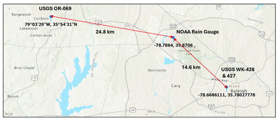
Figure 4. Distances from the NOAA rain gauge at RDU to the USGS wells.

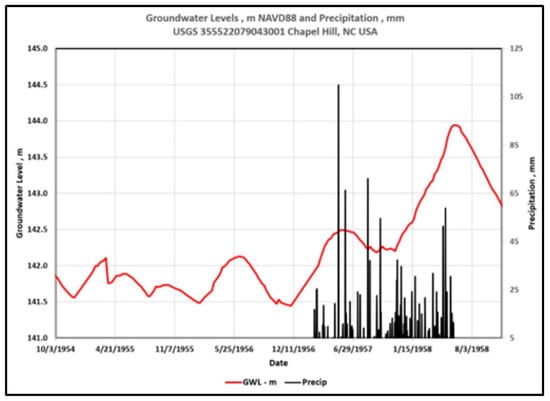
Figure 5. GWL response of the Chapel Hill well to precipitation at RDU.

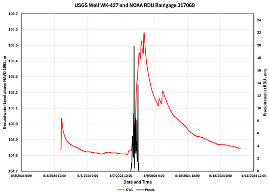
Figure 6. GWL response of the WK-427 Raleigh well to precipitation at RDU.

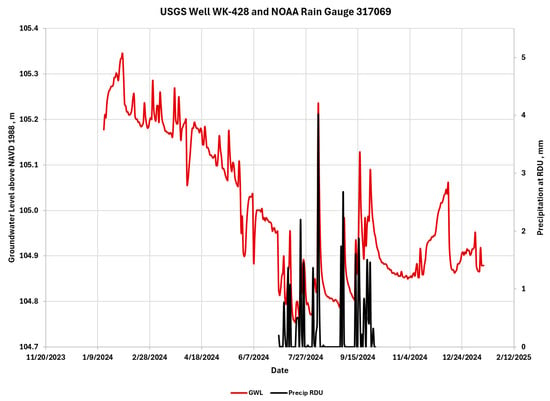
Figure 7. GWL response of the WK-428 Raleigh well to precipitation at RDU.

The locations of the USGS wells at or very near the Fort Lauderdale International Airport (FLL) are illustrated in Figure 8. Their latitudes and longitudes are also listed in Table 1. All of these wells penetrate the Biscayne Aquifer (limestone), illustrated in Figure 9 [14]. The GWL responses of these wells to FLL precipitation are presented in Figure 10. Clearly, there is a well-defined GWL response at each well to the 1–8 June 2017 precipitation event at FLL. Well F-291 (USGS 260010080085001) has a depth of 109 feet (33.22 m), Well G-2147 (USGS 261501080060701) a depth of 46 feet (14.02 m), and Well G-2900 (USGS 260325080113901) a depth of 114.5 feet (34.90 m).

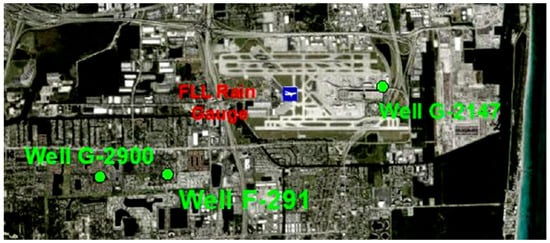
Figure 8. FLL rain gauge and USGS wells.

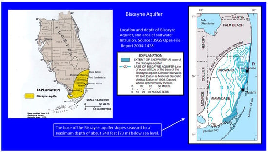
Figure 9. All of the wells penetrate the Biscayne Limestone Aquifer.

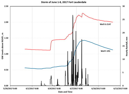
Figure 10. GWL response to precipitation at FLL for Wells G-2147 and F-291.

The locations of the USGS wells at or very near the Miami International Airport (MIA) are illustrated in Figure 11. Their latitudes and longitudes are listed in Table 1, and these wells also penetrate the Biscayne Limestone Aquifer, illustrated earlier in Figure 9 [14]. Wells G-3327 (USGS 254823080163701) and G-3329 (USGS 254752080181501) are 54 feet (16.46 m) deep. Well G-3465 (USGS 254823080175201) is 28.8 feet (8.78 m) deep, while G-3466 (USGS 254834080171601) is 19.5 feet (5.94) deep. Well G-3570 (USGS 254536080172601) is 3.59 km (2.23 mi) south of the NOAA rain gauge at MIA and is 18.7 feet (5.70 m) deep. The GWL responses to MIA precipitation are presented in Figure 12 and Figure 13.

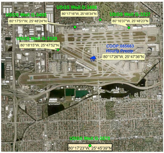
Figure 11. Location of USGS wells and NOAA rain gauge at MIA.

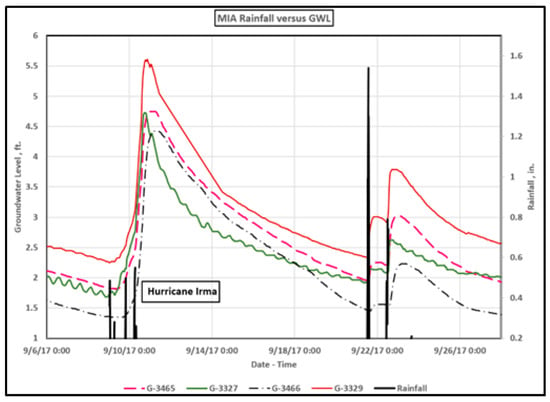
Figure 12. GWL response of each well at the airport to MIA precipitation.

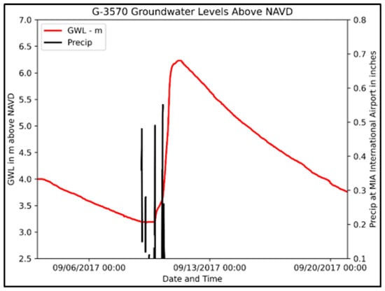
Figure 13. Well G-3570 GWL response to MIA precipitation.

All the USGS wells at the airport respond quickly to MIA precipitation. As shown in Figure 12, the rainfall from Hurricane Irma in 2017 is much smaller than the non-hurricane event that followed in late September. This is quite common in South Florida, where hurricanes are mostly wind events. The GWL response to MIA precipitation at Well G-3570 [3.59 km (2.23 mi) south of the NOAA rain gauge at MIA] is also almost immediate (see Figure 13).

Figure 14 illustrates the location of the Tampa International Airport (TPA) and the closest well (USGS 275843082222201, W.D.Fussell 618 in Table 1), which is 11 miles (17.70 km) east of TPA, completed in the Floridan Aquifer System, with a depth of 69 feet (21.03 m). Their latitudes and longitudes are listed in Table 1. The NOAA rainfall station at TPA is FL 08-8788. The well is characterized as having a short data series (1973–2007), inconsistent measurement sequences, and gaps from year to year. The GWL response from this well to the rainfall at TPA indicates a poor connection (see Figure 15). This will be confirmed in the next section, as the climate trends between the rainfall annual maxima at TPA and the GWL annual maxima do not match.

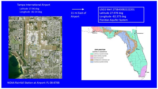
Figure 14. Tampa International Airport and USGS Well 275843082222201.

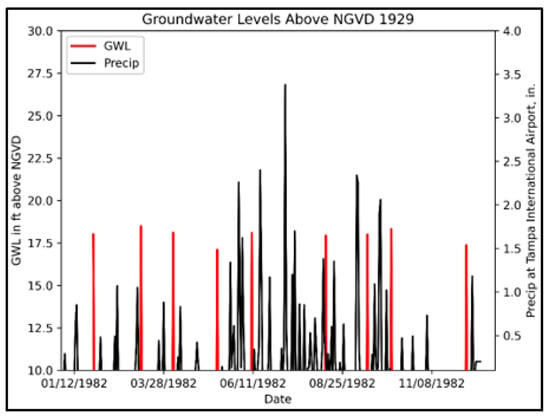
Figure 15. Poor GWL response to precipitation at TPA.

Figure 16 illustrates the location of the Logan International Airport (BOS) and the closest well. MA-BGW 925 (USGS 422133071033801) is 2.56 mi (4.12 km) west of BOS, completed in the “Sediments” (120SDMS) local aquifer with a depth of 624 feet (190.20 km). Their latitudes and longitudes are listed in Table 1. Although the well appears not to be hydrogeologically connected, its GWL response to BOS precipitation shows a good cause-and-effect relationship (see Figure 17).

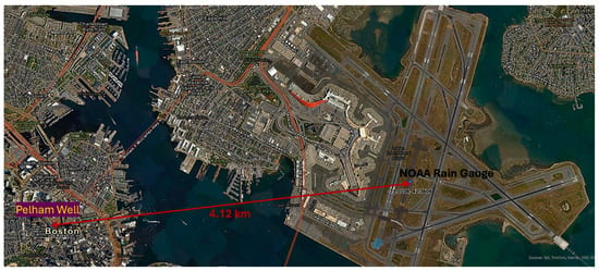
Figure 16. Logan International Airport (BOS) and Well MA-BGW 925 (USGS 422133071033801).

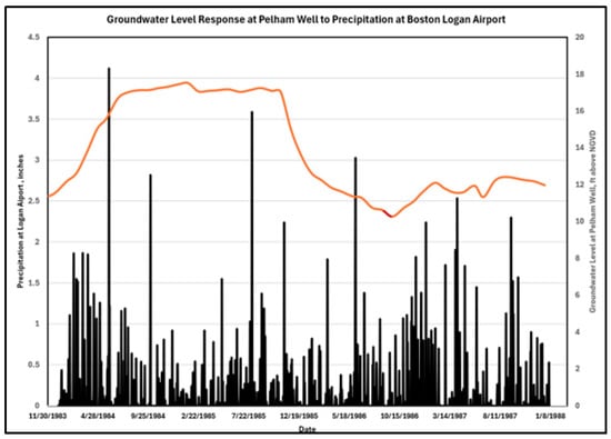
Figure 17. Pelham well GWL response to BOS precipitation.

3.2. Potential Climate Trends

As reviewed in Section 2.1 (Nonstationary Methods for Analyzing Extreme Events), potential climate trends are predicted by applying the generalized extreme value (GEV) distribution to the annual maxima for precipitation and groundwater level response. The methodology includes maximum likelihood estimates (MLEs) of the location (µ) parameters of the GEV, as presented earlier in Equation (1) [9,10,11]. The return levels of nonstationary versus stationary curves for design periods (T) are compared to determine whether they are both increasing or decreasing values. The precipitation annual maxima series (AMS) for 24-h duration events at RDU (NOAA Station 31-7069) is provided by the Precipitation Frequency Data Server (PFDS) for the period of 1945–2000 [13], illustrated in Figure 18. The nonstationary time series return curve is above the stationary time series curve, indicating an increasing-values climate trend. The maximum likelihood estimation (MLE) of the time variable location parameter is listed in Table 2.

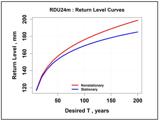
Figure 18. Nonstationary versus stationary time series curves for RDU (AMS 1945–2000).

Table 2. Maximum Likelihood Estimation of RDU GEV Location Parameters.

RDU GEV Location Parameters	Estimation Method Used: MLE 1
Negative Log-Likelihood Value: 349.851
Estimated parameters:
mu0	mu1	scale	shape
67.10071290	0.07914207	20.16447096	0.02822432
Standard Error Estimates:
mu0	mu1	scale	shape
2.7509731	0.1119234	2.0946679	0.1164602
Estimated parameter covariance matrix:
	mu0	mu1	scale	shape
mu0	7.56785295	0.03601434	2.79729262	−0.14646069
mu1	0.03601434	0.01252685	0.03116475	−0.00286548
scale	2.79729262	0.03116475	4.38763366	−0.10570796
shape	−0.14646069	−0.00286548	−0.10570796	0.01356298

¹ Note: Maximum Likelihood Estimation.

The time variable location parameter for the RDU AMS (for 24-h duration) is given by

$$\begin{array}{l}{\mu }_t={\mu }_0+{\mu }_1 t\\ {\mu }_t=67.10+0.079t\end{array}$$

(7)

where µ₀ = 67.10 mm (2.64 in.) of precipitation.

The magnitude of µ₁ (the slope of the linear function) confirms that the nonstationary time series curve in Figure 18 is above the stationary time series curve, indicating that the climate trend values are increasing. As noted earlier in Table 1, the Raleigh wells (WK-427 and WK 428) have very short record lengths, not suitable for climate trend analysis. Therefore, the Chapel Hill NC well (OR-069, USGS 355522079043001) was analyzed for climate trend analysis. The nonstationary versus stationary time series curves are presented in Figure 19. The results match the RDU precipitation time series curves, with the nonstationary curve above the stationary curve.

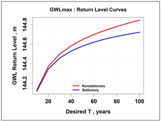
Figure 19. Return level curves for the USGS 355522079043001 well climate trend analysis.

The time variable location parameter for the USGS 355522079043001 well annual maxima MLE is given by

$$\begin{array}{l}{\mu }_t={\mu }_0+{\mu }_1 t\\ {\mu }_t=142.97+0.0015t\end{array}$$

(8)

where µ₀ = 142.97 m (469.06 feet) above the North American Vertical Datum of 1988 (NAVD 88). Table 3 provides further details of the MLE computation.

Table 3. Maximum Likelihood Estimation of Well OR-069 GEV Location Parameters.

Well OR-069 GEV Location Parameters	Estimation Method Used: MLE 1
Negative Log-Likelihood Value: 49.23084
Estimated parameters:
mu0	mu1	scale	shape
142.966295532	0.001543837	0.641078694	−0.271583601
Standard Error Estimates:
mu0	mu1	scale	shape
0.103101235	0.006809236	0.076679174	0.118332447
Estimated parameter covariance matrix.
	mu0	mu1	scale	shape
mu0	1.062986 × 10−2	−8.709549 × 10−5	0.0009746521	−0.0053695923
mu1	−8.709549 × 10−5	4.636570 × 10−5	−0.0001075509	0.0002830358
scale	9.746521× 10−4	−1.075509 × 10−4	0.0058796958	−0.0057615950
shape	−5.369592 × 10−3	2.830358 × 10−4	−0.0057615950	0.0140025680

¹ Note: Maximum Likelihood Estimation.

The RDU–Chapel Hill NC locations are 130–150 miles (209–241 km) from the coastline. Rainfall over coastal urban areas presents unique challenges. The extreme rainfall events tend to be larger, and runoff to the sea and groundwater levels are compounded by sea level rise effects [15]. There are global causes for sea level rise that are independent from local rainfall, for example, water melting from ice sheets in Greenland and Antarctica has a major impact on the global average rise in sea levels. In coastal aquifers, hydraulic heads are also controlled by variations in sea level [16]. Thus, the GWL response for the wells at or near the coastal urban airports is not exclusively due to precipitation. The nonstationary versus stationary return level curves for the FLL AMS precipitation (for 24-h duration events, 1960–2010) at the Fort Lauderdale International Airport (FLL) are illustrated in Figure 20. The results show an increasing-values climate trend for the desired design return periods T.

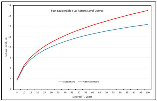
Figure 20. Nonstationary versus stationary curves for FLL precipitation (AMS 1960–2010).

The time variable location parameter for the FLL AMS (for 24-h duration) from the MLE computation is given by

$$\begin{array}{l}{\mu }_t={\mu }_0+{\mu }_1 t\\ {\mu }_t=3.74+0.005t\end{array}$$

(9)

where µ₀ = 3.74 inches (79.76 mm) of precipitation.

The return level curves for the G-2900 well (USGS 260325080113901) climate trend analysis (for 2001–2018 annual maxima) are presented in Figure 21 and match the FLL precipitation climate trend analysis. The time variable location parameter for the G-2900 well computed annual maxima from the MLE computation is given by

$$\begin{array}{l}{\mu }_t={\mu }_0+{\mu }_1 t\\ {\mu }_t=2.37+0.0009t\end{array}$$

(10)

where µ₀ = 2.37 feet above the National Geodetic Vertical Datum of 1929 (NGVD 29). Sea level rise impacts for South Florida are reviewed below. The nonstationary versus stationary return level curves for the NOAA rain gauge historical precipitation AMS (for 24-h duration events, 1937–2010) at the Miami International Airport (MIA) overlap and are presented in Figure 22. They are indistinguishable, as there is no appreciable climate change predicted. The return level curves for the G-3570 well (USGS 254536080172601) at MIA (for 1994–2024 annual maxima) are presented in Figure 23.

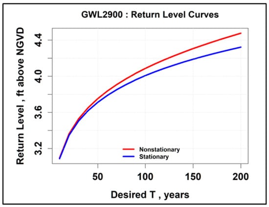
Figure 21. Return level curves for the Fort Lauderdale G-2900 well climate trend analysis.

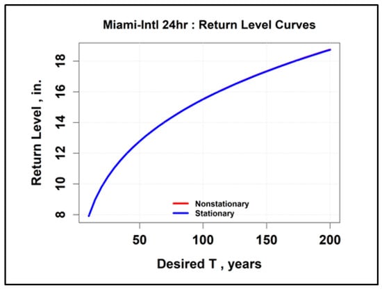
Figure 22. Return level curves overlap: no climate change predicted at MIA (AMS 1937–2010).

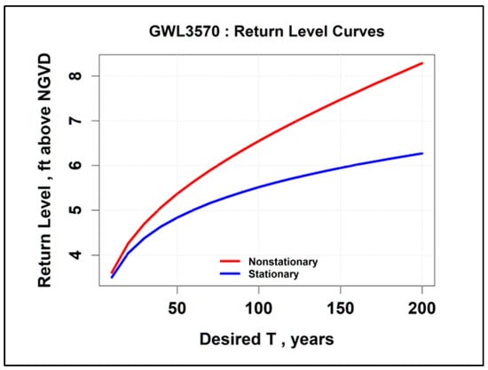
Figure 23. Return level curves for the MIA G-3570 well (USGS 254536080172601).

The time variable location parameter for the G-3570 well (USGS 254536080172601) for the 1994–2024 MLE-computed annual maxima is given by

$$\begin{array}{l}{\mu }_t={\mu }_0+{\mu }_1 t\\ {\mu }_t=2.028+0.012t\end{array}$$

(11)

where µ₀ = 2.028 feet (0.62 m) above NGVD 29. Clearly, the curves in Figure 23 and the equation above confirm a robust increasing-values climate trend unlike the precipitation results in Figure 20 (which were based on the NOAA PFDS time series 1937–2010). A reasonable assumption is that the groundwater level in well G-3570 for 1994–2024 is impacted by sea level rise. The Virginia Key sea level rise monitor is located on Virginia Key, a small island in Biscayne Bay, south of Miami Beach. It is approximately 6.3 miles (10.1 km) from the Miami International Airport (MIA). A relative sea level refers to changes in the sea level at a specific location relative to the local land elevation The relative sea level trend at the Virginia Key location is 3.19 mm/year with a 95% confidence interval of +/− 0.22 mm/yr, based on monthly mean sea level data from 1931 to 2024 [17]. This is equivalent to a change of 1.05 feet (0.32 m) in 100 years: this trend is presented in Figure 24. Undoubtedly, the GWL is impacted by SLR at both the Fort Lauderdale and Miami, FL, wells.

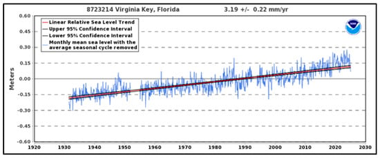
Figure 24. The relative sea level trend at Virginia Key (10 km from MIA).

The return level curves for the NOAA rain gauge recording AMS (24-h duration, 1900–2010) at the Tampa International Airport (TPA) are presented in Figure 25. The results indicate a potential climate trend of decreasing values. Return level curves for climate trend analysis of USGS Well 275843082222201 annual maxima are presented in Figure 26. It was noted in Section 3.1 that there was a poor GWL response to precipitation at TPA at that well, indicating no hydrologic connection. Not surprisingly, the climate trend for the well is reversed from that of the precipitation at TPA. Groundwater levels (GWLs) are in units of feet above the NGVD 1929 datum. Data for (1973–2007) were retrieved from USGS records through a Python script, and annual maxima were computed using another Python script.

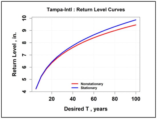
Figure 25. Nonstationary versus stationary time series curves for TPA (AMS 1900–2010).

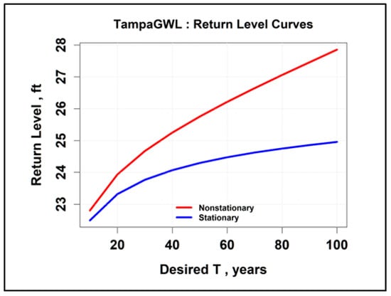
Figure 26. Return level curves for the USGS Well 275843082222201 climate trend analysis.

The time variable location parameter for the USGS Well 275843082222201 annual maxima MLE is given by

$$\begin{array}{l}{\mu }_t={\mu }_0+{\mu }_1 t\\ {\mu }_t=18.22+0.039t\end{array}$$

(12)

where μ₀ = 18.22 feet (5.55 m) above NGVD 29. It also indicates a strong increasing value for µ₁ (slope of the linear function of log-transformed values). Based upon scientific data, the Tampa Bay Climate Science Advisory Panel (CSAP) concludes that the Tampa Bay region may experience sea level rise (SLR) somewhere between 11 inches (0.28 m) to 2.5 feet (0.76 m) in 2050 [18]. Thus, some SLR effects may have been present in the climate trend signal for USGS Well 275843082222201 during the 1973–2007 time period. The nonstationary versus stationary return level curves for the Logan International Airport (BOS) in Boston, Massachusetts, for NOAA AMS (24-h duration, 1900–2013) are presented in Figure 27. The predicted climate trend shows slightly increasing values.

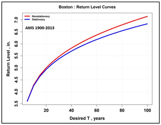
Figure 27. Return level curves for Logan International Airport (BOS) for AMS 1900–2013.

The time variable location parameter for the BOS annual maxima MLE is given by

$$\begin{array}{l}{\mu }_t={\mu }_0+{\mu }_1 t\\ {\mu }_t=2.32+0.002t\end{array}$$

(13)

where µ₀ = 2.32 inches (58.92 mm) of precipitation.

This confirms the slightly increasing nonstationary curve values by examining the magnitude of µ₁. Return level curves for climate trend analysis for the Pelham MA well (MA-BGW 925, USGS 422133071033801) from computed annual maxima are presented in Figure 28.

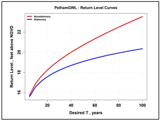
Figure 28. Return level curves for the Pelham MA well climate trend analysis for 1960–1997.

The time variable location parameter for the Pelham well computed-annual-maxima is given by:

$$\begin{array}{l}{\mu }_t={\mu }_0+{\mu }_1 t\\ {\mu }_t=12.34+0.039t\end{array}$$

(14)

where µ₀ = 12.34 feet above NGVD 29. It also confirms the substantially increasing nonstationary curve values by examining the magnitude of µ₁. According to the Commonwealth of Massachusetts SLR profile, by 2070, some projections estimate a rise in sea level of 2.3 to 4.2 feet (0.70 to 1.28 m) over 2000 levels [19].

4. Discussion

The methodology applied in this manuscript does not attempt to describe the physics of the underlying groundwater processes. It has been made quite clear through Figure 1 and Figure 2 that the equations illustrated in these figures have been kept separate from the numbered equations in the manuscript on purpose. Once a groundwater level (GWL) response to precipitation has been established at a particular site, the methodology to predict climate trends for both the rainfall and nearby GWL signals (from the data retrieval of government agency measurements) is strictly a probabilistic approach. These GWL measurements are already a consequence of the hydrogeologic properties of the subsurface and other external factors like sea level rise. Certainly, articles exploring major physical groundwater processes (such as lithological processes, infiltration, transport pathways), geologic controls, and the probabilistic identification of preferential subsurface flow paths are important contributions [20,21].

As noted in Section 2.2, a reliable source of precipitation data is the National Oceanic and Atmospheric Administration (NOAA) NCEI (National Centers for Environmental Information), which actually stores both US and selected foreign country monitoring data. Access to such data is available online, and the longest records tend to be associated with major US airports. Therefore, the first step was to determine whether a reasonable GWL response exists to historical precipitation events at major airports selected for this study, identified in Section 3.1. From Table 1 in Section 2.2, the Raleigh-Durham precipitation record length (for complete years) is 1950–2024. However, it should be emphasized that the annual maxima series provided by the NOAA Precipitation Frequency Data Server (PFDS) is for the time period of 1945–2000 [13]. Although the GWL responses to concurrent RDU precipitation events were good for all the wells, the Raleigh wells (WK-427 and WK-428) have a very short record length, not suitable for climate trend analysis. Therefore, the Chapel Hill NC well, with a record length of 1948–1997, was subjected to extreme value analysis (EVA) and the results show that the nonstationary versus stationary time series agree between the RDU precipitation station (Figure 17) and the well (Figure 18), supported by the maximum likelihood estimation (MLE) computation of the GEV parameters in Section 3.2 (Equations 7 and 8). Furthermore, the Raleigh-Durham area station locations are 130–150 miles (209–241 km) from the coastline and are not impacted by sea level rise (SLR). The elevation of RDU is 436 feet (132.9 m) above mean sea level (MSL), and the elevation of the Chapel Hill well is 511.50 feet (155.91 m) above NGVD 1929.

The elevation of the Fort Lauderdale International airport (FLL) is 65 feet (20 m) above MSL, while the elevation of well G-2900 (USGS 260325080113901) is 5.98 feet (1.82 m) above NGVD 29. The well depth is 114.5 feet (34.9 m) and fully penetrates the unconfined Biscayne Limestone Aquifer. Although the FLL rainfall record length is 78 years, the annual maxima series provided by the NOAA PFDS is for the time period of 1960–2010 [13]. The nonstationary versus stationary time series between the FLL precipitation station (Figure 19) and the well (Figure 20) agree, supported by the maximum likelihood estimation (MLE) computation of the GEV parameters in Section 3.2 (Equations 9 and 10). As noted earlier, Well G-2900 is impacted by SLR, as presented in Figure 23: FLL is 26.9 miles (43.29 km) from MIA and approximately 53 km from the Virginia Key sea level monitoring station. It is not possible to separate the SLR component and the GWL response to precipitation from the EVA in Figure 20.

The elevation of the Miami International Airport (MIA) is 9.843 feet (3 m) above the mean sea level, while the elevation of Well G-3570 (USGS 254536080172601) is 10.3 feet (3.14 m) above NGVD 29. The well depth is 18.7 feet (5.7 m) and also penetrates the unconfined Biscayne Limestone Aquifer. Again, although the MIA rainfall record length is 76 years, the annual maxima series provided by the NOAA PFDS is for the time period of 1937–2010 [13]. Most interestingly, the nonstationary versus stationary return level curves for the NOAA rain gauge precipitation AMS (for 24-h duration events) at MIA overlap (Figure 22); they are indistinguishable, as there is no appreciable climate change predicted. However, the return level curves for the G-3570 well (USGS 254536080172601) at MIA (Figure 23, for 1994–2024 annual maxima) show a robust increasing-values climate trend. As noted in the previous section, a reasonable assumption is that the groundwater level in Well G-3570 for the 1994–2024 period was impacted by sea level rise. As noted in Section 3.2, the global causes for sea level rise (water melting from ice sheets in Greenland and Antarctica) are independent from the local climate. Although not within the scope of this article, it has been noted that it is difficult to differentiate between all the hydrologic variables affecting the groundwater levels under climate change. Certainly, land use changes are also independent of climate change but impact recharge and groundwater levels. These merit further study in the future.

There was a poor GWL response at the Tampa well (USGS 275843082222201) to precipitation at the Tampa International Airport (TPA) for the time period (1973–2007), indicating that no likely hydrologic connection exists (the well is 17.7 km east of TPA). The elevation of TPA is 26 feet (7.9 m) above the MSL and the elevation of the well is 30.50 ft (9.3 m) above NGVD 29 with a depth of 69 feet (21.03 m) above NGVD 29 penetrating the Floridan Aquifer System. Although the Tampa Bay region may experience sea level rise (SLR) somewhere between 11 inches (0.28 m) to 2.5 feet (0.76 m) in 2050 [18], there may have already been SLR impacts during the time period of 1973–2007. The Logan International Airport (BOS) in Boston has an elevation of 19.69 feet (6 m) above MSL, while the well at Pelham (USGS 422133071033801, 4.12 km west of BOS across the bay) is 35 feet (10.7 m) above NGVD 29 with a depth of 624 feet deep (190.19 m) above NGVD 29. Although the well appears not to be hydrogeologically connected (see Figure 16), its GWL response to BOS precipitation shows a good cause-and-effect relationship (see Figure 17). The well not only responds to precipitation at BOS, but the climate trend return level curves for BOS (Figure 27, AMS 1900–2010) agree with the return level curves for the period of 1960–1997 (see Figure 28)). The AMS for 24-h duration storm events reported by the NOAA PFDS for BOS (1900–2013) represents one of the longest such time series.

NOAA Atlas 15 is the new spatially continuous National Precipitation Frequency Atlas of the United States, currently under development by the NOAA National Weather Service (NWS), Office of Water Prediction [22]. NOAA Atlas 15 represents a shift from a stationary assumption to a nonstationary assumption (i.e., extreme precipitation events change over time).

5. Conclusions

Stream–aquifer interactions, as well as surface water/groundwater interactions within wetlands, require a solution of complex partial differential equations of flow and contaminant transport, namely a deterministic approach [1,2]. These deterministic modeling approaches would be impractical for the evaluation of groundwater level responses to long precipitation time series of extreme value events (such as annual maxima) and to subsequently predict potential climate trends. A probabilistic approach is required. At most major US airports, the NOAA maintains precipitation monitoring stations, and data on annual maxima may be obtained through the Precipitation Frequency Data Server (PFDS). Five major airports were selected for precipitation extreme value analysis (EVA) as follows: (1) Raleigh-Durham International Airport, NC (RDU); (2) Fort Lauderdale International Airport, FL (FLL); (3) Miami International Airport, FL (MIA); (4) Tampa International Airport, FL (TPA); and (5) Logan International Airport, MA (BOS). U.S. Geological Survey wells at or near these airports (see Table 1) were reviewed for groundwater level (GWL) response to precipitation. The wells with the longest and error-free data records were selected for EVA after computing their annual maxima series.

The inland stations, the RDU airport and the Chapel Hill NC well (209–241 km from the coastline) at elevations 132.9 m above MSL and 155.9 m above NGVD 1929, respectively, are not impacted by SLR. The GWL response to RDU precipitation is good, and the EVA climate trend for the annual maxima for both stations match (nonstationary curves above the stationary curves). The strongest and practically immediate GWL responses to precipitation were obtained for the wells located at or very near the Fort Lauderdale and Miami airports: these wells penetrate the unconfined Biscayne Limestone Aquifer. Their GWL climate trends matched the airport precipitation climate trends, as verified by maximum likelihood estimates (MLEs) of the GEV parameters. There is evidence that SLR impacts these wells. The Tampa well, 11 miles (17.70 km) east of TPA, penetrates the Floridan Aquifer system and is characterized as having a short data series (1973–2007), with inconsistent measurement sequences and gaps from year to year. The GWL response from this well to the rainfall at TPA indicates a poor hydrologic connection, and the climate trends of both TPA rainfall and the GWL annual maxima do not match. In spite of its short data series, the climate trend prediction is most probably impacted by SLR. Although the Logan International Airport (BOS) and the Pelham well (4.12 km west of BOS) are not hydrogeologically connected, a good GWL response to precipitation at BOS exists. The climate trend EVA for the Pelham well confirms the substantially increasing nonstationary curve values, suggesting that SLR impacts are present.

It has been demonstrated that EVA of the GWL annual maxima series is a useful tool. The strength of the relationship through MLE computation of the GEV parameters reinforces the GWL response to precipitation for individual events. The return level curves of annual maxima for specific return periods, for both the precipitation time series and the GWL, provide another measure of whether these climate trends match. The extreme value analysis of groundwater levels for wells near coastlines also provides at least partial evidence of sea level rise impacts.

References

- Lin, Y.-C.; Medina, M.A., Jr. Incorporating transient storage in conjunctive stream–aquifer modeling. Adv. Water Resour. 2003, 26, 1001–1019. [Google Scholar] [CrossRef]
- Kazezyılmaz-Alhan, C.M.; Medina, M.A.; Richardson, C.J. A Wetland Hydrology and Water Quality Model Incorporating Surface Water/Groundwater Interactions. Water Resour. Res. 2007, 43, 1–16. [Google Scholar] [CrossRef]
- Barnard, P.L.; Befus, K.M.; Danielson, J.J.; Engelstad, A.C.; Erikson, L.H.; Foxgrover, A.C.; Hayden, M.K.; Hoover, D.J.; Leijnse, T.W.B.; Massey, C.; et al. Projections of multiple climate-related coastal hazards for the US Southeast Atlantic. Nat. Clim. Change 2024, 15, 101–109. [Google Scholar] [CrossRef]
- Cortez, N.A.; Esterson, K.; Coronado, C.; Maran, C. Chapter 2B: Water and Climate Resilience Metrics; South Florida Environmental Report; South Florida Water Management District: West Palm Beach, FL, USA, 2023; Volume I, pp. 2B1–2B45. [Google Scholar]
- Obeysekera, J.; Salas, J.D. Quantifying the Uncertainty of Design Floods under Nonstationary Conditions. J. Hydrol. Eng. 2014, 19, 1438–1446. [Google Scholar] [CrossRef]
- Kidmose, J.; Refsgaard, J.C.; Troldborg, L.; Seaby, L.P.; Escrivà, M.M. Climate change impact on groundwater levels: Ensemble modelling of extreme values. Hydrol. Earth Syst. Sci. 2013, 17, 1619–1634. [Google Scholar] [CrossRef]
- Kupfersberger, H.; Rock, G.; Draxler, J.C. Combining Groundwater Flow Modeling and Local Estimates of Extreme Groundwater Levels to Predict the Groundwater Surface with a Return Period of 100 Years. Geosciences 2020, 10, 373. [Google Scholar] [CrossRef]
- Cheng, L.; AghaKouchak, A.; Gilleland, E.; Katz, R.W. Non-stationary Extreme Value Analysis in a Changing Climate. Clim. Change 2014, 127, 353–369. [Google Scholar] [CrossRef]
- Gilleland, E.; Katz, R.W. extRemes2.0: An Extreme Value Analysis Package in R. J. Stat. Softw. 2016, 72, 1–39. [Google Scholar] [CrossRef]
- Gilleland, E.R. Package extRemes—Weather and Climate Applications of Extreme Value Analysis (EVA), extRemes 2.2; U.S. National Oceanic and Atmospheric Administration Internet Source: Washington, DC, USA, 2024. [Google Scholar]
- Gilleland, E.; Ribatet, M.; Stephenson, A.G. A software review for extreme value analysis. Extremes 2013, 16, 103–119. [Google Scholar] [CrossRef]
- Nederhoff, K.; Saleh, R.; Tehranirad, B.; Herdman, L.; Erikson, L.; Barnard, P.L.; van der Wegen, M. Drivers of extreme water levels in a large, urban, high-energy coastal estuary—A case study of the San Francisco Bay. Coast. Eng. 2021, 170, 103984. [Google Scholar] [CrossRef]
- NOAA Precipitation Frequency Data Server (PFDS). Available online: https://hdsc.nws.noaa.gov/pfds/ (accessed on 19 June 2025.).
- Bradner, A.; McPherson, B.F.; Miller, R.L.; Kish, G.; Bernard, B. Quality of Ground Water in the Biscayne Aquifer in Miami-Dade, Broward, and Palm Beach Counties, Florida, 1996–1998, with Emphasis on Contaminants; Open-File Report 2004-1438; U.S. Geological Survey: Reston, VA, USA, 2005; pp. 1–25. [Google Scholar]
- Medina, M.A. Do Record Storm Events Produce Floods of the Same Magnitude? In Engineering Methods for Precipitation Under a Changing Climate; Rolf, O.J., Adamec, K.T., Eds.; ASCE: Reston, VA, USA, 2020; Chapter 2; ISBN 978-0-7844-1552-8. [Google Scholar] [CrossRef]
- Shellie, H.; Fletcher, C.H.; Barbee, M.M.; Fornace, K.L. Hidden Threat: The Influence of Sea-Level Rise on Coastal Groundwater and the Convergence of Impacts on Municipal Infrastructure. Annu. Rev. Mar. Sci. 2024, 16, 81–103. [Google Scholar] [CrossRef]
- NOAA Tides and Currents. Available online: https://tidesandcurrents.noaa.gov/sltrends/plots/8723214_meantrend.png (accessed on 19 June 2025).
- Pinellas County Flood Map Service–Sea Level Rise Map of Tampa Bay. Available online: https://floodmaps.pinellas.gov/pages/sea-level-rise (accessed on 19 June 2025).
- Commonwealth of Massachusetts Sea Level Rise Profile. Available online: https://www.mass.gov/info-details/sea-level-rise (accessed on 19 June 2025).
- Beetle-Moorcroft, F.; Shanafield, M.; Singha, K. Exploring conceptual models of infiltration and groundwater recharge on an intermittent river: The role of geologic controls. J. Hydrol. Reg. Stud. 2021, 35, 100814. [Google Scholar] [CrossRef]
- Schiavo, M.; Riva, M.; Guadagnini, L.; Zehe, E.; Guadagnini, A. Probabilistic identification of Preferential Groundwater Networks. J. Hydrol. 2022, 610, 127906. [Google Scholar] [CrossRef]
- NOAA Atlas 15: Update to the National Precipitation Frequency Standard. Available online: https://water.noaa.gov/about/atlas15 (accessed on 19 June 2025).
Disclaimer/Publisher’s Note: The statements, opinions and data contained in all publications are solely those of the individual author(s) and contributor(s) and not of MDPI and/or the editor(s). MDPI and/or the editor(s) disclaim responsibility for any injury to people or property resulting from any ideas, methods, instructions or products referred to in the content. |
© 2025 by the author. Licensee MDPI, Basel, Switzerland. This article is an open access article distributed under the terms and conditions of the Creative Commons Attribution (CC BY) license (https://creativecommons.org/licenses/by/4.0/).