Experimental Study of Wave Overtopping Flow Behavior on Composite Breakwater

Abstract

The safety of pedestrians on a breakwater structure or seawall is significantly influenced by two essential factors: the wave overtopping flow velocity (OFV) and the overtopping layer thickness (OLT). The main issue, however, is that most studies have predominantly focused on impermeable structures rather than composite breakwaters. This study conducted 55 physical experiments to investigate the OFV and OLT on a composite breakwater. The non-intrusive bubble image velocimetry (BIV) technique was employed to measure the OFV and OLT, as well as the plunging distance on the rear side of the structure. Empirical equations with two sets of dimensionless variables, the wave steepness and relative crest freeboard, were proposed as predictors. The results show that these two dimensionless variables perform well for both OFV and OLT estimation. The comparison between the proposed empirical equation and the available empirical equation in the literature is also presented. Finally, the proposed empirical equations were used to estimate the maximum instantaneous wave overtopping discharge and plunging distance. The findings of this research offer insights into the physical mechanisms of wave overtopping, providing an initial exploration into the design of composite breakwaters.

1. Introduction

The velocity of wave overtopping flow (referred to as OFV) and the thickness of the overtopping layer (referred to as OLT) are two critical parameters that require careful consideration, especially when prioritizing the safety of pedestrians on a breakwater or seawall. Elevated OFV values give rise to fast-moving wave overtopping flows, while thick OLT further exacerbates the risk of pedestrians being swept off the breakwater [1]. Furthermore, the presence of harbor oscillations [2,3] as well as storms [4] potentially amplifies the wave overtopping hazards. A comprehensive understanding of both the OFV and OLT is essential to ensure the safety of pedestrians on breakwater structures. By comprehending these parameters and implementing suitable design considerations and mitigation strategies, the potential risks can be effectively minimized.

The study of pedestrian safety usually involves examining human subjects’ failure mechanisms and investigating wave overtopping flow properties. Human instability resulting from wave overtopping flow can be categorized into two types: tumbling, where the moment from the current exceeds the moment produced by human weight, and slipping, where the current forces exceed the friction force between the shoes and the ground. Various wave overtopping flow properties, such as wave overtopping discharge, wave overtopping volume [5,6], wave forces [7,8], and the products of OLT and OFV [1,9,10,11,12], have been used as limiting factors for human instability. Furthermore, EurOtop [5] suggests that the wave overtopping plunging distance is a parameter that exposes hazards to structures, pedestrians, and vehicles.

In the early studies, the wave overtopping flow was simulated using flood flow, where the water depth and velocity were gradually increased until the subject lost stability [9,10,11]. This flood flow exhibits different characteristics compared to wave overtopping, where the flow is transient. Bae et al. [1] conducted a physical experiment aimed at examining human stability under wave overtopping flow on a vertical breakwater crest. They used a threshold based on the products of OLT and OFV, which were measured from wave overtopping flow, as a means of assessing stability. The study revealed that the failure of human stability, manifested as tiptoe lifting and slipping/tumbling, occurred at lower values compared to studies involving steady flow or flooding. Specifically, failures were observed in cases characterized by a shallow OLT and high OFV, indicating high speed and shallow wave overtopping flow. Sandoval and Bruce [12] analyzed videos of wave overtopping hazards and estimated the critical values of OLT and OFV that cause human instability. They compared their findings to the available critical values from the literature, which were obtained through physical experiments using flood flows. Similar to Bae et al. [1], Sandoval and Bruce [12] also found that the critical OLT values in real wave overtopping flows were shallower compared to the ones obtained from flood flow conditions. Additionally, the critical value of OFV from wave overtopping flow was also higher. This highlights the importance of considering actual wave overtopping conditions when assessing human stability.

EurOtop [5] established tolerable overtopping limits for structures, properties, and the safety of people and vehicles. They used the mean overtopping discharge and the individual maximum overtopping volume as parameters for wave overtopping flow. For the safety of individuals on breakwaters, they recommend a maximum individual wave overtopping volume of $V<$ 600 l/m, while the wave overtopping discharge limits range from 0.3 to 20 l/s per m depending on the wave height. This limit was later confirmed in the study by Cao et al. [7], where they studied human instability resulting from wave overtopping flow. In the accompanied study [8], they identified inline forces as the critical factor for human instability and emphasized the importance of OLT and OFV in estimating wave forces.

The accurate estimation of wave overtopping flow properties is crucial for ensuring pedestrian safety. The OLT and OFV can also be used to estimate the wave overtopping volume, discharge, and force. Therefore, obtaining precise estimates of the OLT and OFV during breakwater design is critical. The characteristics of overtopping flows and the associated hazards depend on the structure’s geometry and wave conditions. While the interaction between wave overtopping flow and human instability has been studied, the focus on OLT and OFV has primarily been on impermeable structures like sea dikes [13,14,15,16], with limited research conducted on breakwaters or seawalls.

Mares-Nassare et al. [17] initially studied wave overtopping parameters on rubble mound breakwater structures. They employed wave breaking conditions and three types of armor units: one-layer Cubipod, two-layer cube, and two-layer rock. Using a micro propeller and wave gauge, they measured the wave overtopping parameters, OFV, and OLT at the middle crest of the breakwater. In their research, they applied and calibrated available empirical equations originally developed for sea dikes [5,14,18]. The study was further expanded upon in the work by Mares-Nassare et al. [19], where they examined the influence of two different foreshore slopes on the OLT and OFV at the middle of the breakwater crest, utilizing the same breakwater configuration and wave conditions. The findings indicated a decrease in the OLT and a slight increase in the OFV with increasing foreshore slope values. Additionally, new empirical equations were proposed through Neural Networks (NNs) [20]. The study revealed that the relative crest freeboard played a significant role in estimating the OLT, while the Iribarren number emerged as a significant variable in estimating the OFV [20].

Conventionally, the OFV and OLT are measured using velocity meters and wave gauges [13,17,21,22,23]. Despite being widely used instruments, measuring the OFV and OLT with these instruments is challenging due to the turbulent and aerated nature of the wave overtopping flow [14,22]. Another instrument for velocity measurement, such as the Acoustic Doppler Velocimeter (ADV), requires the continuous (not intermittent) submersion of the instrument [24]. These challenges present opportunities for exploring measurements of wave overtopping parameters. Ryu et al. [25] developed a flow measurement technique called bubble image velocimetry (BIV). In this technique, the flow movement is recorded using a high-speed camera. By analyzing the displacement of the bubbles’ pattern within the flow, the velocity can be determined. BIV has been used in studies of wave breaking [26,27] and wave overtopping [28,29]. Furthermore, digital imaging can be employed to detect the water surface for the OLT [8].

Our previous studies [30,31] investigated the OFV and OLT on a composite breakwater using the BIV technique. A composite breakwater is a type of breakwater where the structure has an armor layer at the front and back, while the middle is constructed with concrete, allowing for pedestrian access along the crest. Therefore, studying the OFV and OLT for this composite-type breakwater is essential. Only the relationship between the OFV and wave and structure conditions has been investigated in our previous study [30]. The application of available empirical equations developed for dikes in estimating the OFV and OLT on a composite breakwater is presented in [31]. However, there are no empirical equations developed specifically for the OFV and OLT on a composite breakwater.

In this paper, we reanalyze the data from our previous studies [30,31] to provide new empirical equations for the estimation of the OFV and OLT on the composite breakwater. Through the dimensional analysis, two sets of dimensionless variables, the wave steepness and crest freeboard, were developed as the estimators of the OFV and OLT. We hypothesize that these newly developed empirical equations will yield more accurate estimations of the OFV and OLT, thus enhancing our understanding of wave overtopping on composite breakwaters.

This paper is organized as follows: In Section 2, we first present a summary of the available studies on the OFV and OLT for breakwaters. Following that, we discuss the dimensional analysis conducted to derive the dimensionless variables that influence the OFV and OLT. Subsequently, we detail the experimental setup and measurement methods. Section 3 examines the relationship between the dimensionless variables, compares them with existing formulas, and presents the application of the proposed empirical equation. Section 4 provides an interpretation of the results. Finally, in Section 5, we draw our conclusions.

2. Materials and Methods

2.1. Literature Review

As previously stated, the existing studies on wave overtopping parameters found in the literature predominantly concentrate on impermeable structures like sea dikes. There are only a limited number of studies in the literature that have explicitly focused on the wave overtopping flow parameters on breakwaters. In this section, the available studies on wave overtopping parameters (OFV and OLT) on breakwaters are presented. Readers can also refer to Appendix A for a summary of the equations presented in this subsection.

EurOtop [5] provides a methodology for estimating the wave overtopping flow parameters on structures with a permeable slope, under fully irregular wave conditions. The estimation of the OFV and OLT relies on the fictitious wave run-up height ($R_u$) defined at a 2% exceedance under irregular waves, as depicted in Figure 1. The estimation of $R_u$ is based on the wave conditions at the structure’s toe and the structure’s geometry,

$$\frac{R_u}{H}=1.65·{\gamma }_b·{\gamma }_f·{\gamma }_{\beta }·\xi$$

(1a)

with a maximum of

$$\frac{R_u}{H}=1.00·{\gamma }_{fsurging}·{\gamma }_{\beta }\left(4.0-\frac{1.5}{\sqrt{{\gamma }_b·\xi }}\right)$$

(1b)

where ξ is the Iribarren’s number, calculated as $\xi =\frac{\tan \alpha }{\sqrt{2\pi H/g{T}^2}}$, where α represents the structure’s front slope, $T$ is the wave period, and $H$ is the wave height at the structure’s toe. ${\gamma }_f$ is the roughness coefficient that depends on the type of armor, ${\gamma }_b$ is the influence factor for berms, and ${\gamma }_{\beta }$ is the factor that considers the effect of oblique wave attack. For $\xi \ge$ 1.8, the roughness factor ${\gamma }_{fsurging}$ for surging conditions increases linearly up to 1 for $\xi =$ 10:

$$y_{fsurging}={\gamma }_f+\left(\xi -1.8\right)·\left(1-{\gamma }_f\right)/8.2$$

(1c)

This indicates that as the wave becomes longer, it will be less influenced by the roughness of the slope, resulting in a larger amount of water overtopping the structure. EurOtop [5] provides the values of ${\gamma }_f$ for different types of armor units based on the irregular wave study by Bruce et al. [32].

Figure 1. Schematic representation of various wave run-up and wave overtopping parameters.

Figure 1. Schematic representation of various wave run-up and wave overtopping parameters.

The wave run-up velocity ($u\left(z_A\right)$) and wave run-up layer thickness $\left(h_t\left(z_A\right)\right)$, which are the wave run-up parameters, can be estimated using the following formula proposed by Schüttrumpf and van Gent [14]:

$$u(z_A)=c_{A,u}\left(\sqrt{g\left(R_u-z_A\right)}\right),$$

(2)

$$h_t\left(z_A\right)=c_{A,h}\left(R_u-z_A\right),$$

(3)

where $c_{A,u}$ and $c_{A,h}$ are empirical coefficients, as listed in

Table 1. Empirical coefficients in Equations (2), (3) and (6).

Authors	${\mathit{R}}_{\mathit{c}}/\mathit{H}$	$\mathit{V}/\mathit{H}$	${\mathit{c}}_{\mathit{A},\mathit{u}}$	${\mathit{c}}_{\mathit{A},\mathit{h}}$	${\mathit{c}}_{\mathit{c},\mathit{h}}$
van Gent [23]	0.7–2.2	1/4	1.30	0.15	0.40
Schüttrumpf et al. [33]	0.0–4.4	1/3, 1/4, 1/6	1.37	0.33	0.89
van der Meer et al. [15]	0.7–2.9	1/3	0.35cot$\alpha$	0.19	0.13
EurOtop [5]	-	-	1.4, 1.5	0.20, 0.30	–
Mares-Nasarre et al. [17]	0.34–1.75	2/3	–	0.52	0.89
Adibhusana et al. [31]	0.6–1	1/1.5	1.21	0.21	–

, $z_A$ indicates the vertical distance from the still water level, as illustrated in Figure 1, and $g$ represents the acceleration due to gravity. If $R_u$ exceeds the crest freeboard, $R_c$, water will surge over the structure, resulting in wave overtopping. The wave overtopping parameters at the seaward edge of the structure can be estimated by applying Equations (2) and (3), denoted as $u(z_A=R_c)$ and $h_t(z_A=R_c)$.

On the structure crest, EurOtop [5] suggests estimating the OFV along the structure crest ($u\left(x_c\right)$) using Equation (4) following van der Meer et al. [15]:

$$\frac{u\left(x_c\right)}{u\left(z_A=R_c\right)}=\exp \left(-1.4\frac{x_c}{L}\right),$$

(4)

where $L$ is the wavelength and $x_c$ represents the horizontal distance from the intersection of the crest and seaward slope. According to EurOtop [5], the OLT along the crest is typically 2/3 of the OLT at the seaward crest edge:

$$h_t\left(x_c\gg 0\right)=\frac{2}{3}{h}_t(z_A=R_c).$$

(5)

The empirical equations ($c_{A,u}$ and $c_{A,h}$) proposed by van Gent [23], Schüttrumpf et al. [33], van der Meer et al. [15], as well as in EurOtop [5] were derived based on experiments where the structure had an impermeable slope (sea dike). Therefore, calibration is needed if one wants to apply the equations to different structural conditions. Moreover, a study by Molines and Medina [34] shows that the value of ${\gamma }_f$ in Equation (1) also needs to be calibrated. Mares-Nassare et al. [17] conducted physical experiments involving a rubble mound breakwater with a permeable core and a front slope of $V/H=$ 2/3. They used three different armor unit types: a 1-layer Cubipod, a 2-layer cube, and a 2-layer rock. The depth-induced wave breaking near the breakwater model (0.20 $\le H/h\le$ 0.73) and conditions of $\xi =$ 3 or 5 and 0.34 $\le R_c/H\le$ 1.75 were used during the experiment. The experiment involved measurements of the OFV and OLT in the central section of the breakwater. For the estimation, they used Equation (1) to estimate $R_u$ on the rough permeable slope and used Equation (5) to estimate the $h_t(z_A=R_c)$ at the seaward edge of the breakwater. The OLT in the middle of the breakwater was subsequently estimated using Equation (6) [14]:

$$\frac{h_t\left(x_c\right)}{h_t(z_A=R_c)}=\exp \left(-c_{c,h}\frac{x_c}{B}\right).$$

(6)

where $c_{c,h}$ is the empirical coefficient given in Table 1 and $B$ is the structure crest width, as shown in Figure 1. The value of ${\gamma }_f$ was calibrated for each armor unit type, and the empirical coefficients $c_{A,h}$ and $c_{c,h}$ were also calibrated. As a result, an improvement in the estimation was obtained compared to using the available empirical coefficients in the literature. They proposed a new ${\gamma }_f$ for each armor unit (${\gamma }_f=$ 0.33, 0.35, and 0.48 for 1-layer Cubipod, 2-layer cube, and 2-layer rock, respectively) and empirical coefficients $c_{A,h}$ and $c_{c,h}$, as shown in Table 1. Equation (7) was subsequently employed to estimate the OFV at the middle of the breakwater [18]:

$$u\left(x_c\right)=K\sqrt{\mathrm{g}{h}_t\left(x_c\right)},$$

(7)

where the value of $K$, which is an empirical coefficient dependent on the type of armor, is as follows: $K$ = 0.57 for 1-layer Cubipod, 0.60 for 2-layer cube, and 0.47 for 2-layer rock.

In their initial study, Mares-Nassare et al. [17] solely estimated the OLT from wave and structure conditions, whereas the OFV was estimated using the measured OLT. In a subsequent study [20] they explored OFV and OLT estimation using Neural Network techniques. The study employed the same mound breakwater geometry and incorporated three distinct armor units. The experiment incorporated two foreshore slope values, $m=$ 1/50 and 1/25, and a wider range of dimensionless freeboard conditions 0.29 $\le R_c/H\le$ 1.77. Four explanatory variables—foreshore slope $m$, dimensionless crest freeboard $R_c/H$, Iribarren’s number $\xi$, and relative depth $h/H$—were proposed as influencers on OLT and OFV. Employing Feedforward Neural Networks, the study investigated the correlation between these explanatory variables and wave overtopping parameters. Based on their analysis, they proposed the following equations for OLT and OFV estimation:

$$\frac{h_t}{H}=C_1+C_{2}m+C_3\left(\frac{R_c}{H}-1\right)+C_4\xi +C_5\frac{h}{H}\ge 0,$$

(8)

$$\frac{u}{H/T}=D_1+D_{2}m+D_3\left(\frac{R_c}{H}-1\right)+D_4{\xi }^2+D_5\frac{h}{H}\ge 0,$$

(9)

The empirical coefficients, $C_1$ to $C_5$ and $D_1$ to $D_5$, are listed in

Table 2. Empirical coefficients for Equation (8).

Armor Layer	${\mathit{C}}_1$	${\mathit{C}}_2$	${\mathit{C}}_3$	${\mathit{C}}_4$	${\mathit{C}}_5$
Cubipod-1L	0	$-$4	$-$1/3	0.095	$-$0.03
Cube-2L	0	$-$2	$-$0.3	0.085	$-$0.02
Rock-2L	1/3	$-$10	$-$0.45	0.080	$-$0.03

and

Table 3. Empirical coefficients for Equation (9).

Armor Layer	${\mathit{D}}_1$	${\mathit{D}}_2$	${\mathit{D}}_3$	${\mathit{D}}_4$	${\mathit{D}}_5$
Cubipod-1L	2	20	$-$2	0.20	$-$1
Cube-2L	4	$-$30	$-$2	0.20	$-$1
Rock-2L	2	$-$30	$-$2	0.20	$-$0.5

, respectively. As we can see in Equation (8), the four explanatory variables have a linear relationship with the dimensionless OLT ($h_t/H)$. Conversely, in Equation (9), the only non-linear (quadratic) relationship is observed with the $\xi$ term, while the other three explanatory variables maintain a linear relationship with the dimensionless OFV ($u/\left(H/T\right))$. Through their analysis, it was found that OLT is primarily influenced by $R_c/H$, while OFV’s primary influencing factor is $\xi$.

Adibhusana et al. [31] conducted a study on OFV and OLT for a composite breakwater with a front slope $V/H=$ 1/1.5, consisting of a 2-layer tetrapod armor unit with a permeable core (see Figure 4 for a sketch of the structure). The range of 0.6 $\le R_c/H\le$ 1 was considered, along with a non-breaking regular wave having 2.79 $\le \xi \le$ 7.22 during the experiment. To estimate the OFV and OLT at the rear edge of the breakwater, Equations (1)–(5) [5] were employed. The ${\gamma }_f$ and $c_{A,u}$ values were calibrated using the method outlined in [17] based on the measured OFV experimental data. Subsequently, using the newly calibrated ${\gamma }_f$ value, estimations for OLT were performed. The proposed values were ${\gamma }_f=$0.35 for the 2-layer tetrapod, $c_{A,u}=$ 1.21, and $c_{A,h}=$ 0.21. The study showcased an enhancement in the estimation accuracy of both OFV and OLT when compared to using available empirical coefficients.

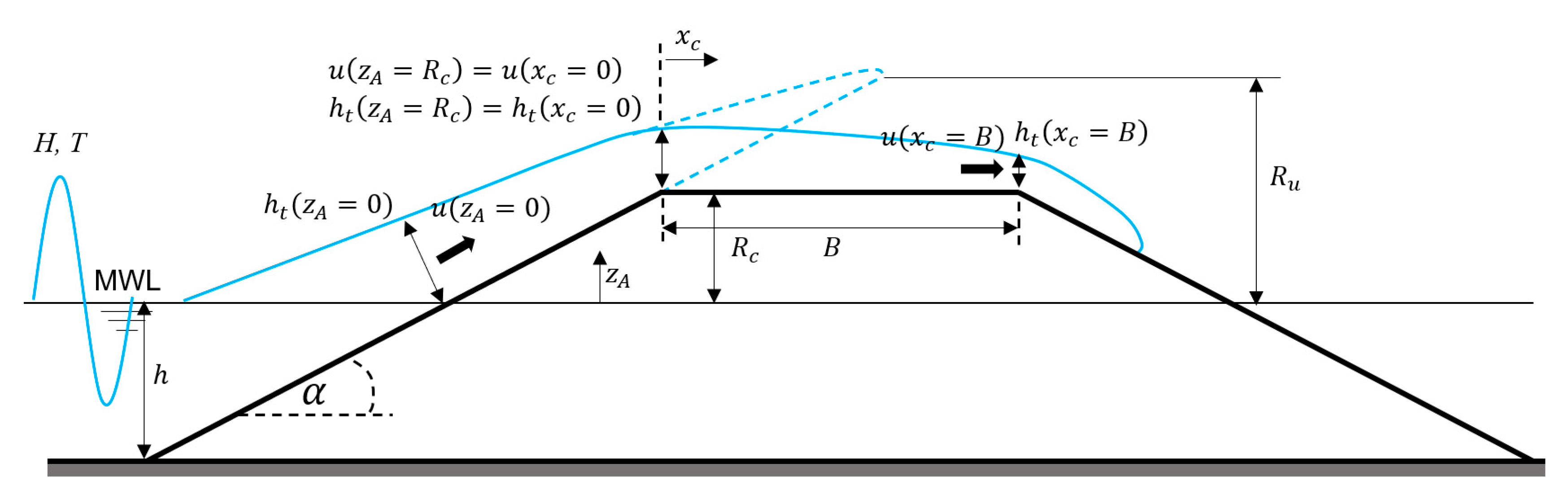
2.2. New Wave Overtopping Estimator

In this paper, we re-analyze experiment data that were previously published. Our previous study used existing empirical equations to estimate wave overtopping parameters [30,31]. However, that approach required several steps and just resulted in minor improvements. In contrast, in this study, we developed a new set of empirical equations for estimating wave overtopping parameters.

This section provides a dimensional analysis for determining the OFV and OLT at the rear edge of the breakwater. These two wave overtopping flow parameters depend on the wave conditions at the structure toe and the structure geometry. The OFV, $u$, at the breakwater crest is influenced by the wave conditions at the structure toe and the structure geometry:

$$u=f(H,T,g,R_c,h,B,\alpha )$$

(10)

where the wave height $H$, the wave period $T$, and the water depth $h$ are the wave conditions. The structure geometry variables are the crest freeboard $R_c$, the crest width $B$, and the structure front slope $\alpha$, as well as the gravitational acceleration $g$. A sketch of these variables are shown in Figure 1.

This system is governed by two fundamental dimensions: length and time. Applying the Buckingham $\pi$ theorem, the system’s behavior is defined by six dimensionless variables. The variables $g$ and $H$ were selected as the repeating variables, resulting in the following six dimensionless variables:

$${\mathsf{\Pi }}_1=\frac{u}{\sqrt{gH}}, {\mathsf{\Pi }}_2=\frac{{gT}^2}{H}, {\mathsf{\Pi }}_3=\frac{B}{H}, {\mathsf{\Pi }}_4=\frac{h}{H}, {\mathsf{\Pi }}_5=\frac{R_c}{H}, {\mathsf{\Pi }}_6=\alpha .$$

(11)

${\pi }_3$ is the dimensionless crest width which defines the location on the structure crest. In this study, the measurement location for OFV was fixed at the rear edge of the structure crest due to safety concerns and limited accessibility on the seaside; hence, ${\pi }_3$ is removed from the analysis. ${\pi }_4$ represents the dimensionless water depth, which is commonly used as a breaking index to indicate whether waves are depth-limited or not. Since the waves in our study are non-breaking, ${\pi }_4$ is not relevant and thus excluded. Regarding ${\pi }_6$, it represents the structure front slope, which could have an impact on the wave overtopping flow. Additionally, the roughness of the armor may also influence the wave overtopping parameters. However, in this research, our main focus lies on investigating the influences of incident wave and wave overtopping characteristics. Given that, in practical scenarios, variations in the angles of the front slope of breakwaters are minimal, and the analysis of overtopping (refer to EurOtop [5]) indicates little deviation for slopes ranging between 1:1.3 and 1:1.2; we opted to exclude the front slope as a parameter in our analysis. Consequently, ${\pi }_6$ is omitted from the study. As a result, the dimensionless analysis is simplified to Equation (12),

$$\frac{u}{\sqrt{gH}}=\varphi \left(\frac{2\pi H}{{gT}^2},\frac{R_c}{H}\right)$$

(12)

indicating that the OFV depends on the wave steepness $2\pi H/{gT}^2$ and the relative crest freeboard $R_c/H$. Note that a constant factor of $2\pi$ was added into the ${\pi }_2$ term, as wave steepness is generally expressed as $2\pi H/{gT}^2$.

The same set of variables was used to establish a set of dimensionless variables for OLT, $h_t$, at the rear edge of the breakwater crest:

$$\frac{h_t}{H}=\varphi \left(\frac{2\pi H}{{gT}^2},\frac{R_c}{H}\right).$$

(13)

Thus, using the same dimensionless variables, both OFV and OLT can be estimated.

Equation (12) differs from the empirical equation we previously proposed in Adibhusana et al. [30]. In our prior study, we used only the relative crest freeboard as the estimator, while the OFV was normalized with the wave celerity, $c$ ($c=L/T$). In this study, the normalized OFV yields a Froude number, which represents the ratio of inertia and gravitational force. The wave steepness and relative crest freeboard are employed as the estimators, leveraging these non-dimensional numbers that are widely used in wave overtopping studies. Additionally, OLT was not analyzed in our prior study [30]; we used the available empirical equation for dikes to estimate OLT [31]. Therefore, Equation (13) represents the new equation for estimating OLT on a composite breakwater. Figure 2 illustrates the procedure for evaluating the proposed Equations (12) and (13) in this study.

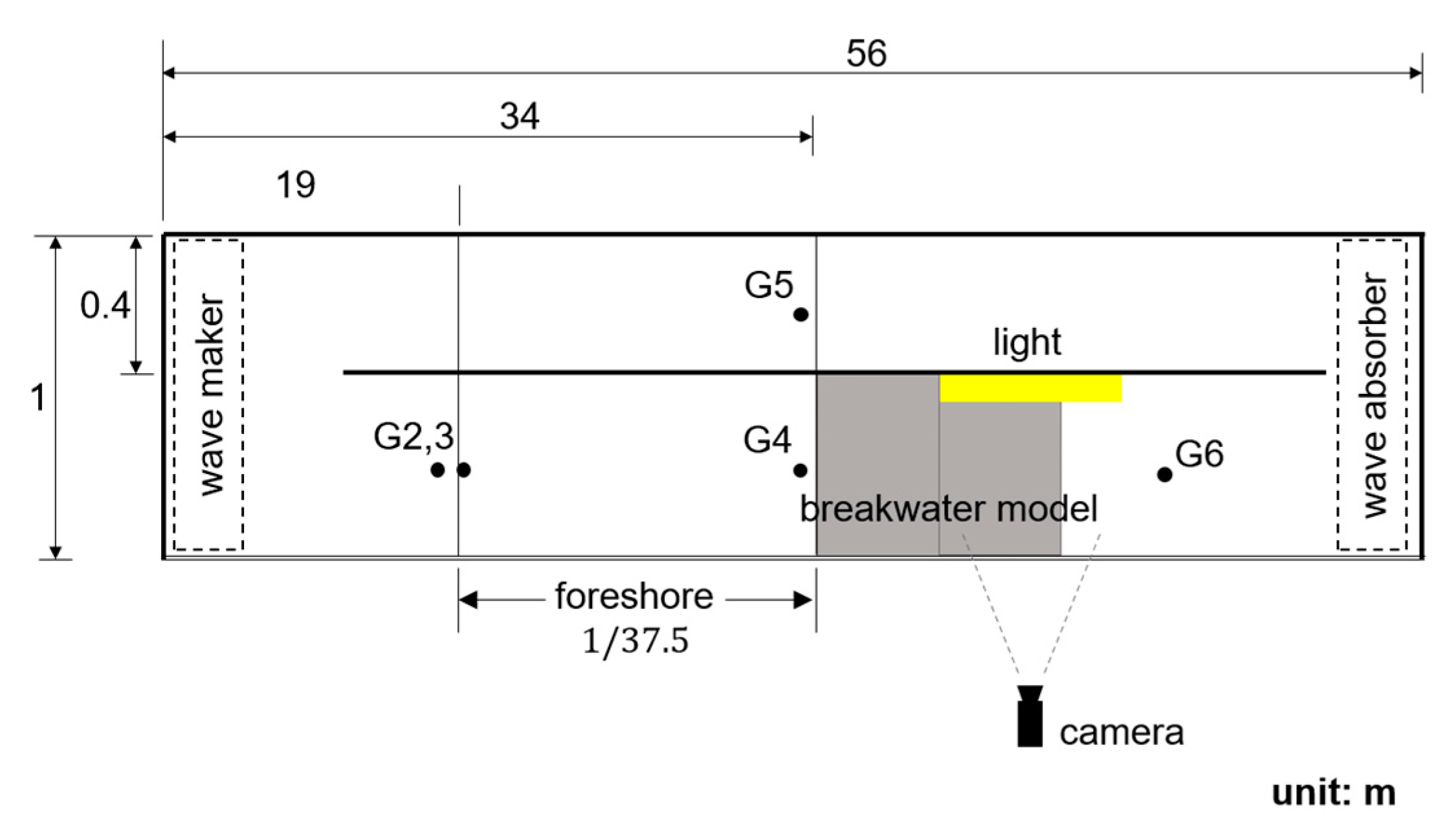
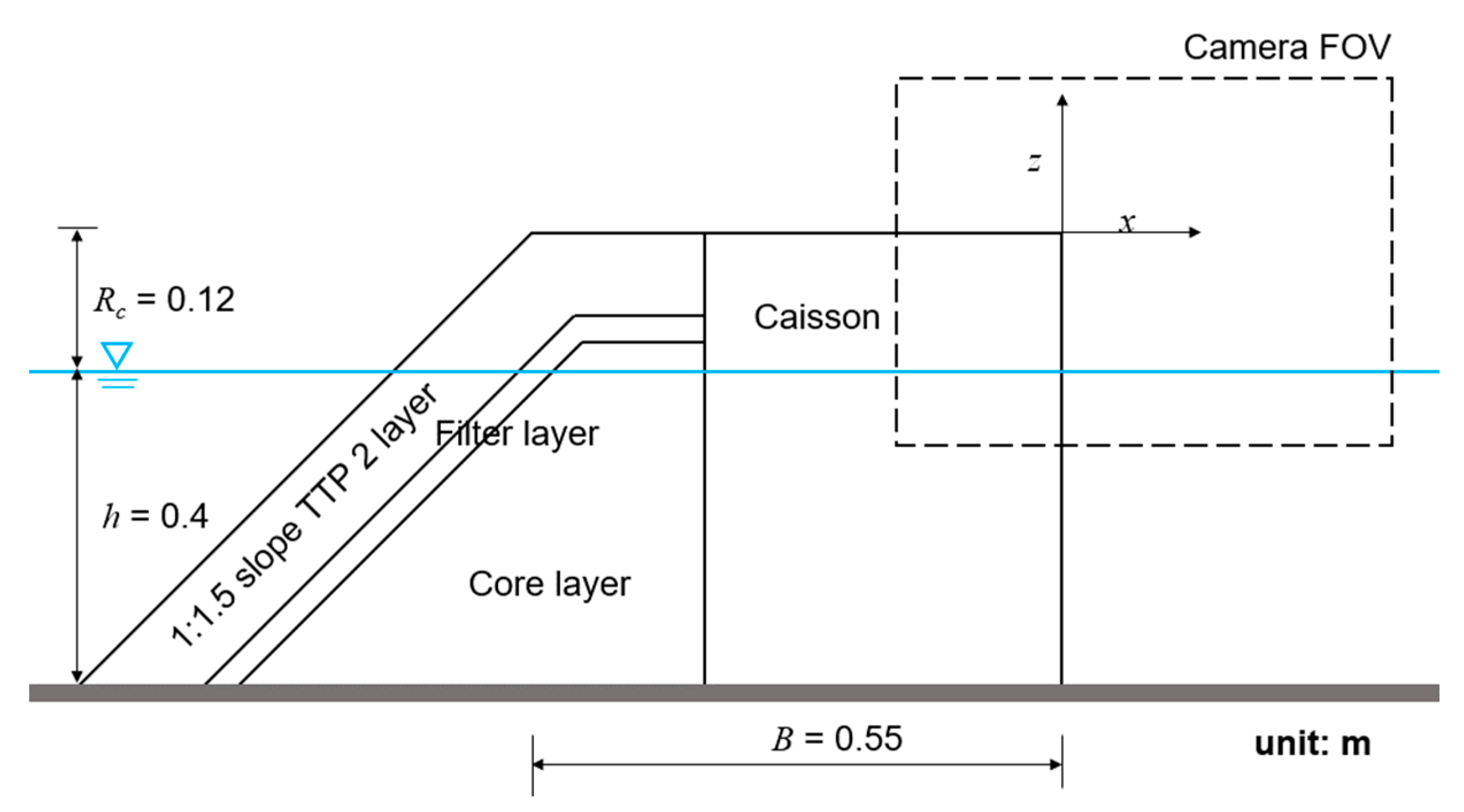
2.3. Setup of the Experiments

In this study, we used the same setup and methodology as described in our previous study [30,31]. This ensured consistency in the experimental conditions, allowing for a direct comparison between the results obtained using the existing empirical equations in our previous study and the new empirical equations proposed in this paper.

The physical model tests were conducted in a two-dimensional wave flume with dimensions of 56 m in length, 1 meter in width, and 2 m in height, which featured a transparent side wall. The wave flume was equipped with a piston-type wave maker capable of generating both regular and irregular waves. The wave maker is also equipped with an active wave absorption system. At the opposite end of the wave flume, a passive wave absorption system was installed to minimize wave reflections. The foreshore, featuring a slope of 1/37.5, is positioned at a distance of 19 m from the wave maker, while a flat bottom is situated 34 m away from the wave maker. The wave flume is divided into two sections: a narrow and a wide section. The breakwater model was positioned 34 m from the wave maker in the wide section. The narrow section was dedicated to measuring water wave conditions without the influence of the structure [35], as shown in Figure 3, illustrating the layout of the wave flume used in this study.

A composite breakwater (scale 1/40) with a front slope, $V/H=$1/1.5, was armored with a 2-layer tetrapod. Quarry stones were used as the filter layer, and the permeable core was made of small quarry stones. In the middle section of the breakwater, a caisson made from acrylic was used. The height of the caisson and armored front slope was the same, making the total height of the breakwater 0.52 m. The water depth at the location of the structure was maintained at a constant value of $h=$ 0.4 m, resulting in a crest freeboard of the breakwater, $R_c=$ 0.12 m. At the end of the breakwater section, there was no armored slope structure, allowing for the wave overtopping to flow freely into the rear side of the breakwater. Figure 4 depicts the schematic representation of the composite breakwater employed in this study.

2.4. Measurement Instruments

In this study, several parameters were measured, including the free water surface elevation, wave overtopping flow velocity, wave overtopping layer thickness, and wave overtopping plunging distance. The measurement setup involved the installation of five capacitance wave gauges within the wave flume, as illustrated in Figure 3. Specifically, two wave gauges, G2 and G3, were positioned 19 m from the wave maker to measure the water surface elevation in deep water. Additionally, another pair of wave gauges, G4 and G5, was located 34 m from the wave maker to capture the water surface elevation at the breakwater toe. Lastly, a wave gauge denoted as G6 was situated behind the breakwater to measure the water elevation behind the structure.

The measurements of wave overtopping flow velocity, wave overtopping layer thickness, and wave overtopping plunging distance were conducted using bubble image velocimetry (BIV) [25]. The BIV setup configuration is depicted in Figure 3. A high-speed camera was positioned perpendicular to the breakwater model. The camera was precisely oriented to capture the wave overtopping flow as it passed and plunged into the rear side of the breakwater, indicated by the camera’s field of view (FOV) in Figure 4. For more about the BIV setup used in this study, additional details can be found in references [30,31].

2.5. Test Conditions

Table 4. Test conditions.

Description	Parameter	Ranges
Wave period	$T$	1.5–3.0 s
Wave height	$H$	0.12–0.20 m
Relative water depth	$h/L$	0.028–0.114
Wave steepness	$H/L$	0.008–0.057
Iribarren’s number	$\xi$	2.795–7.216
Relative crest freeboard	$R_c/H$	0.6–1

summarizes the wave and structure conditions in this study. In this study, a total of 55 regular waves, each with varying wave heights ($H$) and wave periods ($T$), were employed. Regular waves were used as they allowed for a direct analysis of the relationship between wave conditions and wave overtopping flow parameters. This approach is important when designing a specific structure to withstand extreme wave conditions or assessing safety on a breakwater crest. These wave components were representative of various wave conditions, including storm conditions. $H$ and $T$ were measured at the breakwater toe. $H$ was in the range of 0.12–0.20 m and $T$ was in the range of 1.5–3.0 s. The relative water depth $h/L$ in this study, which was in the range of 0.028–0.144, leads to intermediate to shallow water waves. The wave steepness in this study was in the range of $0.008<H/L<0.057$, which was the non-breaking wave condition. The breaker parameter or Iribarren’s number, which was in the range of $2.795<\xi <7.216$, results in plunging to surging wave conditions. The crest freeboard of the structure fell within the range of $0.6<R_c/H<1$.

During these experiments with regular waves, the breakwater reflected a portion of the wave energy, and these reflected waves, in turn, experienced re-reflection toward the breakwater. The wave absorption system was generally able to maintain the wave height; but, due to residuary wave reflection, a long wave was observed. This long wave led to "wave riding", where the short wave rode on the long wave, thus varying the effective water level, increasing the local wave height and/or reducing the freeboard. To obtain reliable measurements, it was essential to establish a specific time frame, excluding the unstable portion of the initial wave and the leading edge of the re-reflected wave reaching the breakwater. In this study, the valid measurement time was defined as the period between the arrival of the first fully developed wave and the arrival of the first re-reflected wave at the breakwater’s toe. This approach ensured that the measurements of wave overtopping parameters, specifically OFV and OLT, remained unaffected by wave reflection. The comparison of free surface elevations from G4 and G5 allowed for the selection of available wave components in proximity to the target wave for analysis.

3. Results

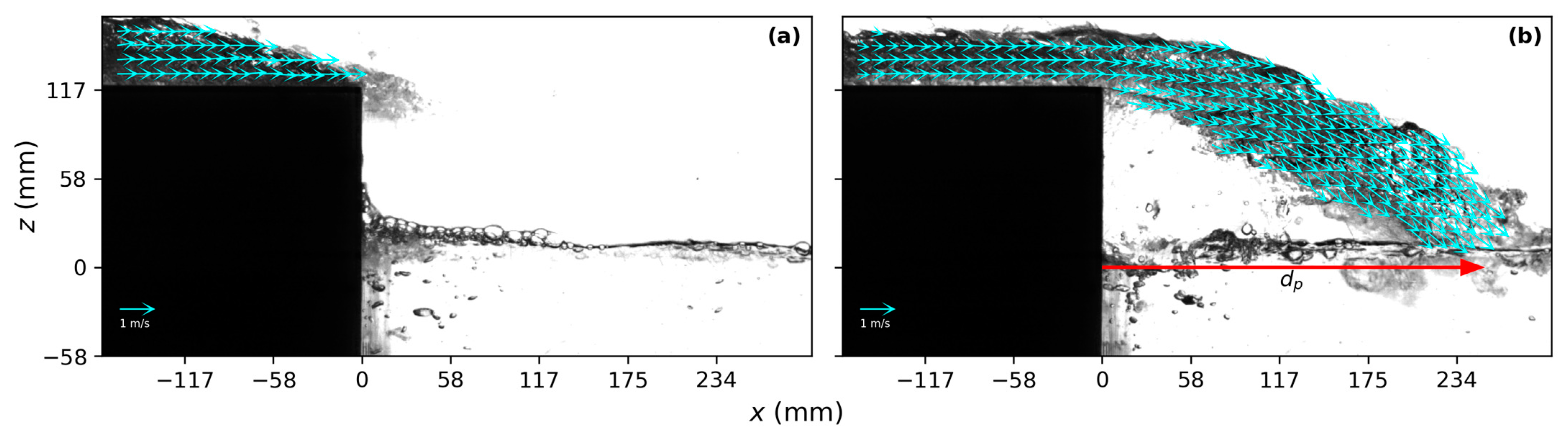
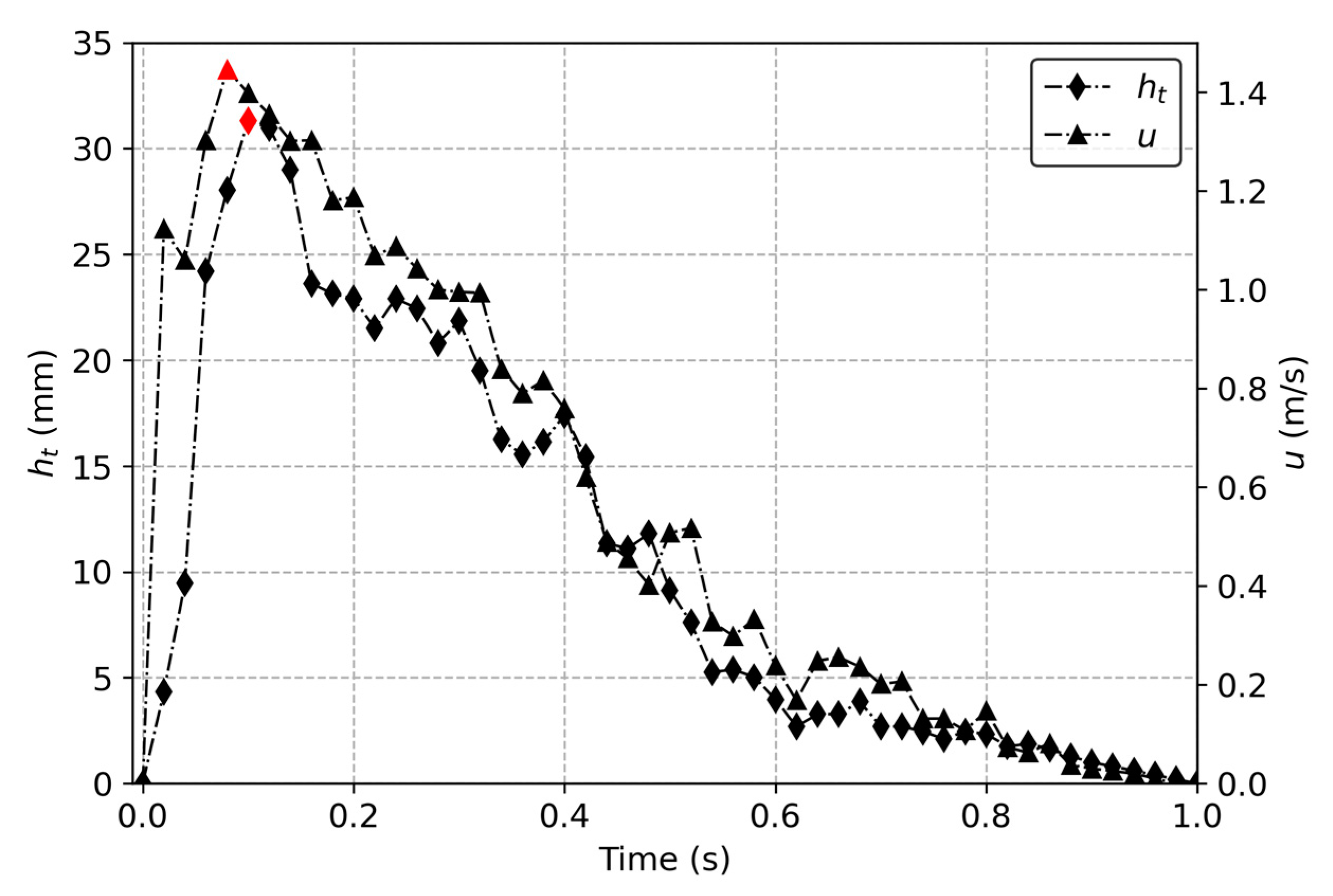
3.1. Flow Pattern of the Overtopping Flow

As previously indicated, the wave overtopping parameters, including the wave overtopping flow velocity, wave overtopping layer thickness, and wave overtopping plunging distance, were measured utilizing the BIV technique. Figure 5 shows an example of a wave overtopping velocity map. Figure 5a shows the wave overtopping reaching the rear edge of the breakwater. The wave overtopping flows are horizontally dominant, as indicated by the velocity vector. The depth-averaged horizontal velocity at the rear edge of the breakwater (i.e., at $x=-0.5$ mm) was extracted from the velocity map. The overtopping layer thickness at this location was obtained by manually digitizing the water surface from the digital image [8]. The time series of both parameters are plotted in Figure 6. As depicted in Figure 6, the wave overtopping flow velocity experiences a rapid increase and eventually reaches its maximum value, which is denoted by a red marker in the plot. The overtopping layer thickness shows a similar pattern; however, the value gradually increases relatively, and the maximum occurs after the maximum overtopping flow velocity. In this study, the maximum velocity and layer thickness were used for the analysis in the next section. From Figure 5a, the sharp front of the overtopping flow can be observed, and the thickest layer follows right after the front. Figure 5b, at the moment right before the wave overtopping hits the water surface, also shows the thickest layer after the front. In Figure 5b, the horizontal distance between the middle of the plunging jet and rear caisson ($x=0$ mm), as shown by the red line, was determined as the wave overtopping plunging distance $d_p$. This parameter was also obtained by carefully digitizing the digital image to identify the midpoint of the plunging jet.

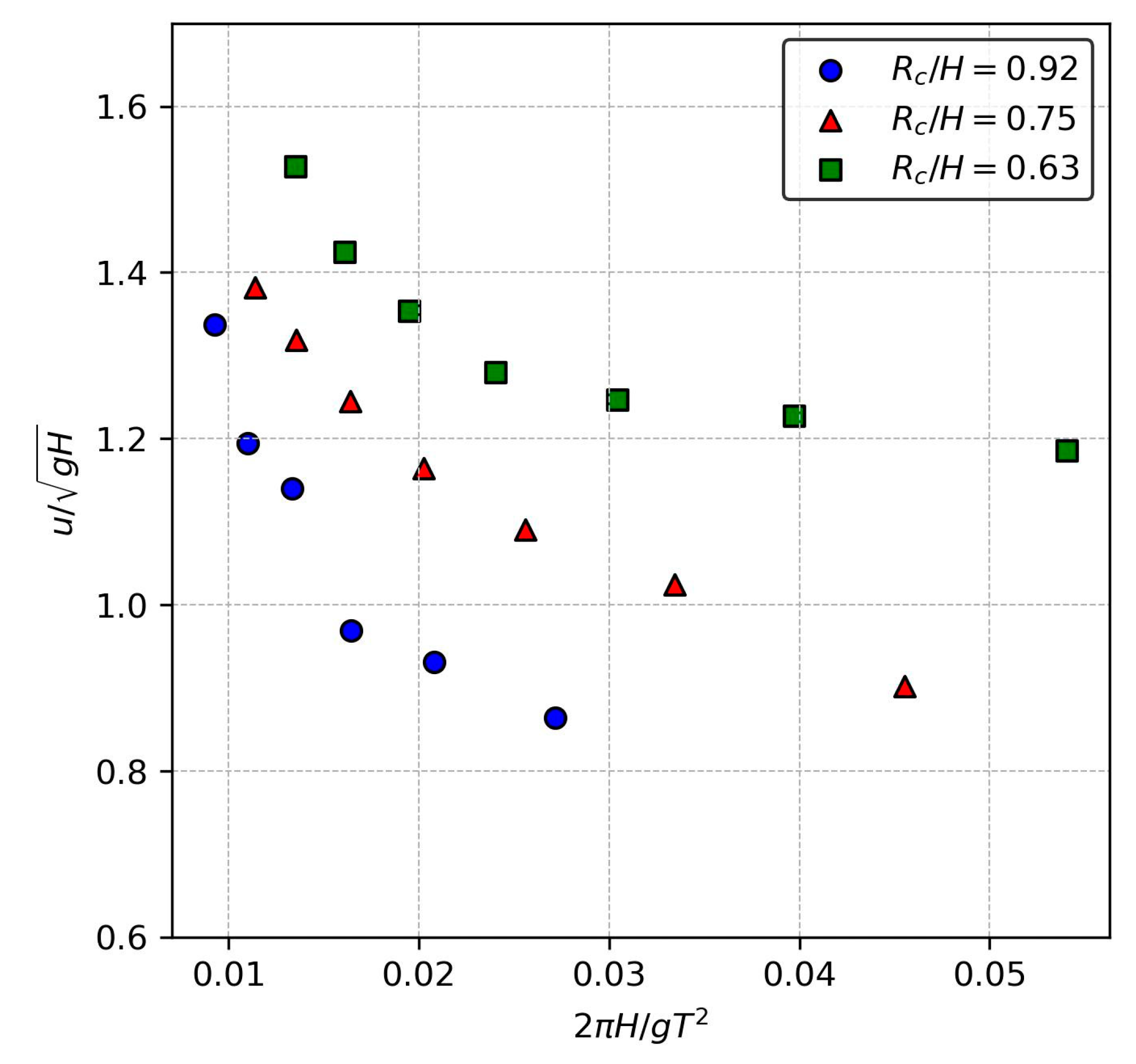
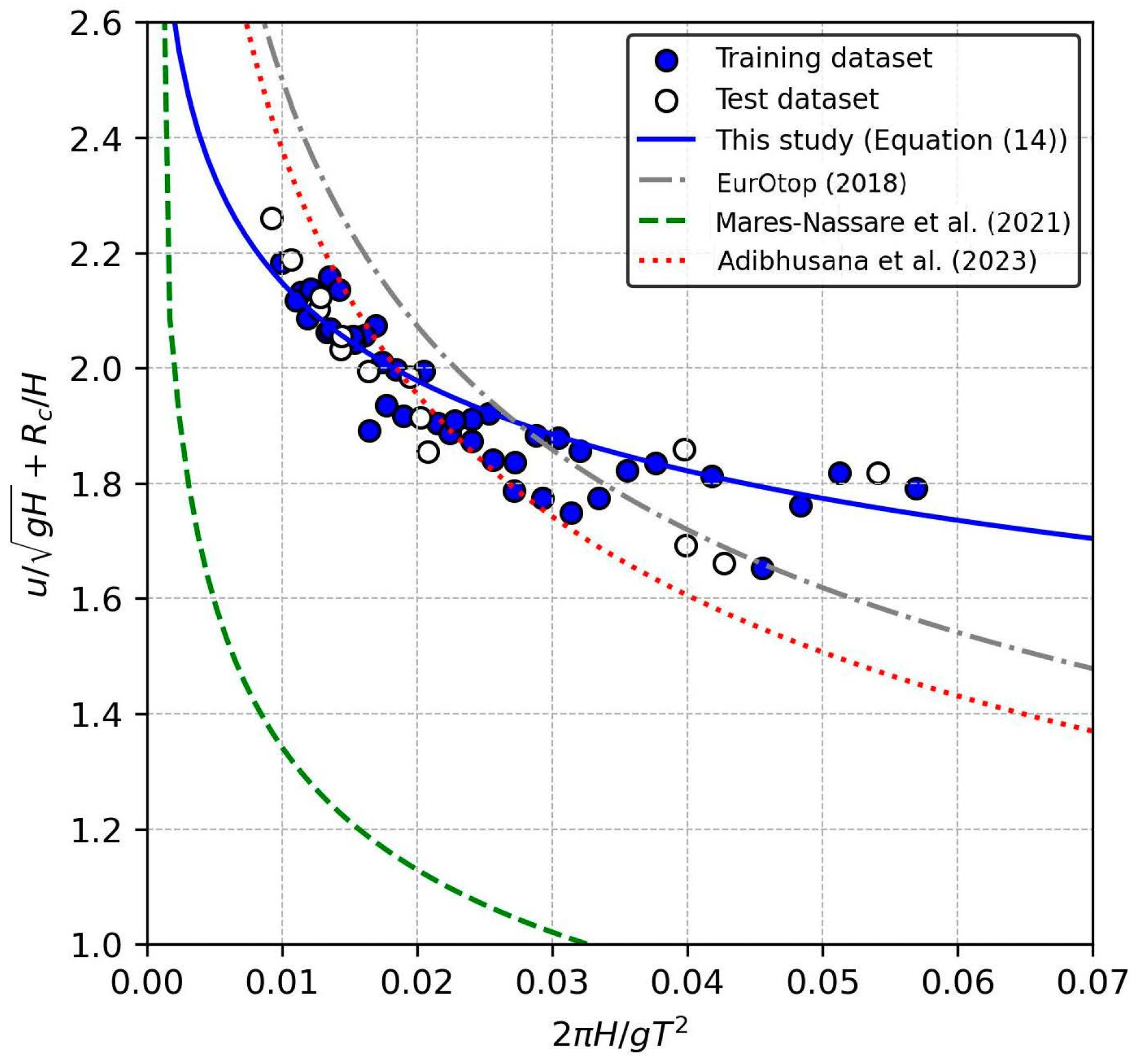
3.2. Overtopping Flow Velocity

In this section, we conduct an analysis of the relationship between the dimensionless variables in Equation (12), using the experimental data for OFV (overtopping flow velocity) estimation. Figure 7 shows the distribution of the dimensionless wave overtopping flow velocity, $u/\sqrt{gH}$, in different wave steepness levels, $2\pi H/g{T}^2$, and relative crest freeboard, $R_c/H$. Figure 7 demonstrates that $u/\sqrt{gH}$ exhibits a linear relationship with $R_c/H$ and a power relationship with $2\pi H/g{T}^2$. The term $R_c/H$ signifies the vertical separation between the crest of the breakwater and the still water level. It acts as a limiting factor for wave overtopping, where higher values of relative crest freeboard result in reduced wave overtopping, and vice versa. This linear relationship was selected to account for the proportional impact of $R_c/H$ on the wave overtopping parameters. $2\pi H/g{T}^2$ is a parameter indicative of the wave’s steepness and its potential for breaking, representing the ratio of $H$ to the wave period $T$. As $2\pi H/g{T}^2$ increases, waves are more prone to breaking. The power relationship was selected to capture this non-linear behavior, where the increase in $2\pi H/g{T}^2$ leads to a significant change in the wave overtopping parameters. A similar pattern and relationship were also observed in other study [20].

Based on this observation, Equation (14) was proposed to model the relationship between the dimensionless variables in Equation (12):

$$\frac{u}{\sqrt{gH}}=a_u{\left(\frac{2\pi H}{g{T}^2}\right)}^{n_u}+b_u\frac{R_c}{H}$$

(14)

A non-linear least squares method was used to fit Equation (14) with the experimental data. To prevent overfitting, we partitioned the experimental data into a training dataset (75%) and a testing dataset (25%). The training dataset was used to determine the optimal empirical coefficients, while the testing dataset was employed to assess the performance of Equation (14) on unseen data. The coefficients $a_u=$ 1.330, $n_u=-$0.136, and $b_u=-$1.416 were determined, and Equation (14) is depicted in Figure 8 alongside the training and testing datasets.

As depicted in Figure 8, Equation (14) aligns well qualitatively with both the training and testing datasets. Coefficients of determination ($R^2$) and relative bias ($bias$) were used to evaluate the accuracy of the proposed empirical equation. A detailed explanation of these two equations can be found in Appendix B. A high agreement was observed with $R^2=$ 0.955 and $bias=$ 0.001 between the training dataset and Equation (14). Similarly, in the testing dataset, a good agreement was obtained with $R^2=$ 0.920 and $bias=$ $-$0.010. These results indicate that $2\pi H/g{T}^2$ and $R_c/H$ are relevant variables for accurately estimating the OFV.

As discussed in Section 2.1, only a few equations are available to estimate OFV on permeable structures. In this section, the available empirical equations in the literature for OFV estimation are plotted in Figure 8 to assess their performances in the present study’s conditions. In the EurOtop [5] equations (Equations (1), (2) and (4)), the roughness factor ${\gamma }_f=$ 0.38 for the two-layer tetrapod, and the empirical coefficient $c_{A,u}=$1.30 [23] were used. The value of $c_{A,u}=$1.30 [23] was used because it gives the best estimation to the present study’s conditions. Noting that the EurOtop [5] equations and empirical coefficient were derived for impermeable structures, their application to the permeable structures considered here may well lead to overestimates. In our previous study, Adibhusana et al. [31], we used the EurOtop [5] equations to estimate the OFV, and we calibrated ${\gamma }_f$ and $c_{A,u}$. As shown in Figure 8, an enhancement of the estimation was obtained. Mares-Nassare et al. [20] developed their equation for rubble mound breakwater using three armor units: two-layer rock, two-layer cube, and one-layer Cubipod. As shown in Figure 8, a poor performance was obtained compared to the EurOtop [5] equations. The poor performance could be due to different armor units giving different reductions to the wave run-up height and, as a result, leading to different wave overtopping values. The detailed quantitative evaluation of each equation’s performance in estimating the OFV is presented in

Table A3. Quantitative performance between empirical equations in OFV estimation.

Author	Training Dataset		Test Dataset
	${\mathit{R}}^2$	$\mathit{b}\mathit{i}\mathit{a}\mathit{s}$	${\mathit{R}}^2$	$\mathit{b}\mathit{i}\mathit{a}\mathit{s}$
This study (Equation (14))	0.955	0.001	0.920	$-$0.010
Adibhusana et al. [31]	0.735	$-$0.026	0.714	$-$0.005
Mares-Nassare et al. [20]: 2-Layer rock 2-Layer cube 1-Layer Cubipod	$<$0.000 $<$0.000 $<$0.000	$-$0.704 $-$0.728 $-$0.762	$<$0.000 $<$0.000 $<$0.000	$-$0.698 $-$0.727 $-$0.761
EurOtop [5]	0.701	0.077	0.695	0.100

of Appendix B.

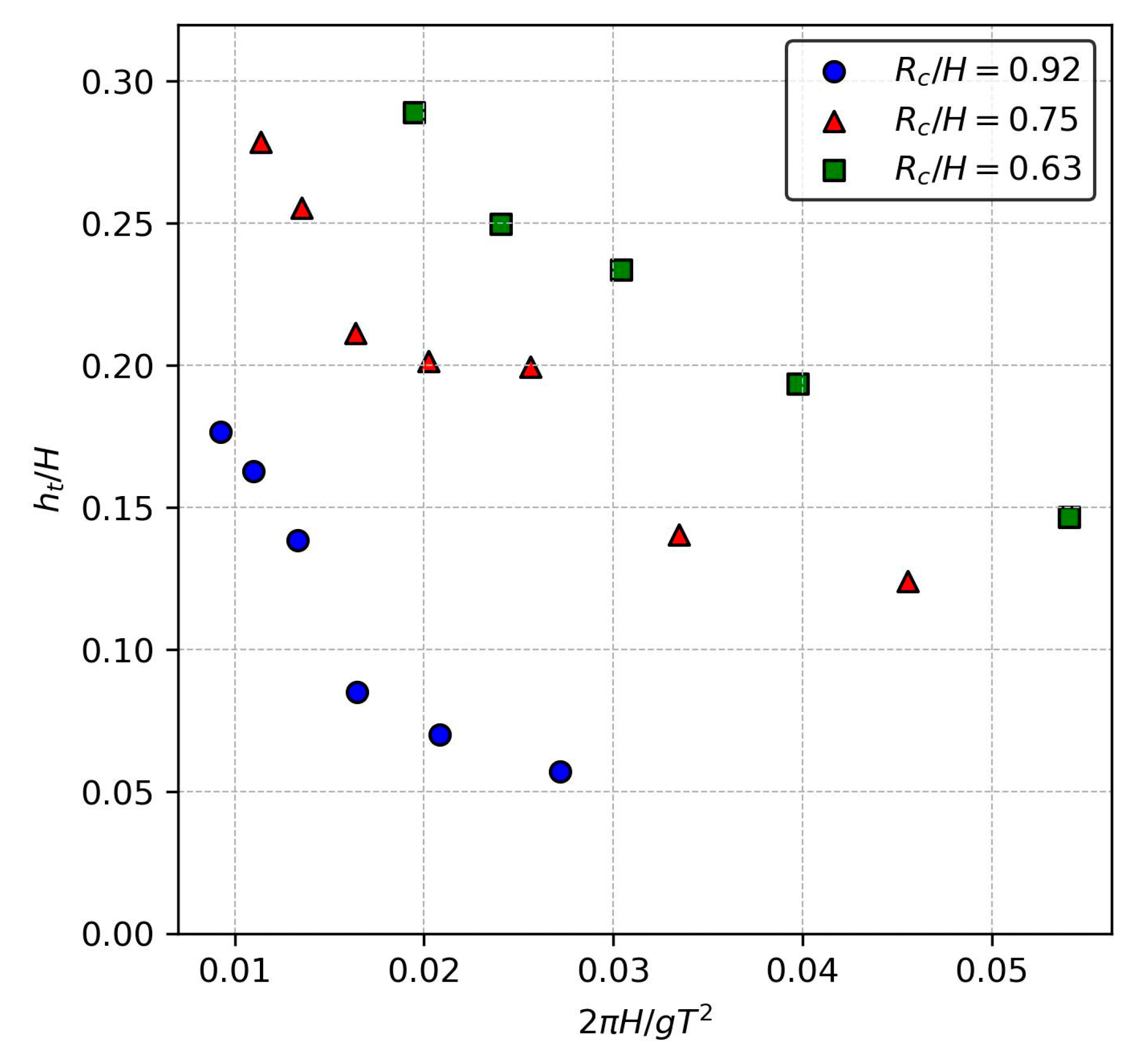
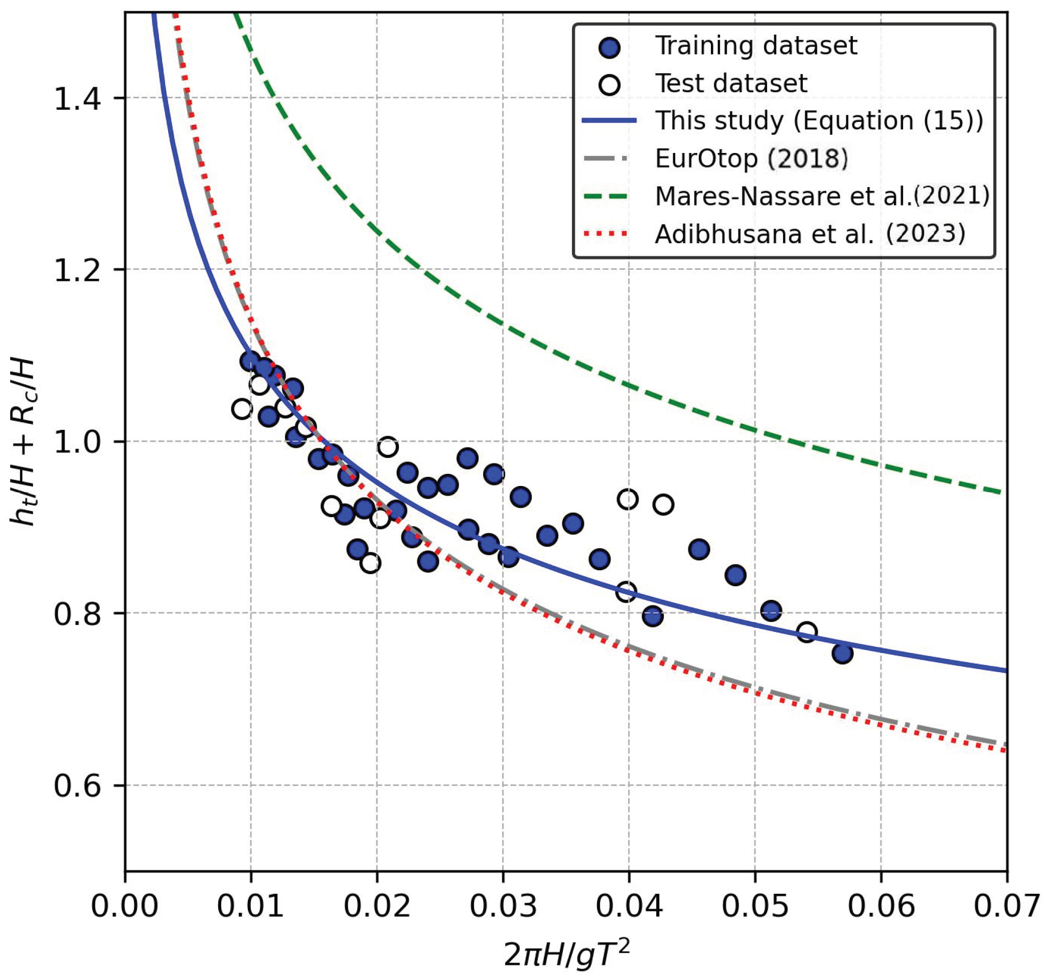
3.3. Overtopping Layer Thickness

In this section, an investigation was carried out to determine the relationship between the dimensionless variables in Equation (13) using the experimental data for estimating the overtopping layer thickness (OLT). Figure 9 displays the distribution among the dimensionless OLT ($h_t/H$), the wave steepness ($2\pi H/g{T}^2$), and the relative crest freeboard ($R_c/H$). From Figure 9, it is evident that $h_t/H$ exhibits a linear relationship with $R_c/H$ and a power relationship with $2\pi H/g{T}^2$, similar to the OFV relationship. Based on this observation, Equation (15) is proposed as the empirical equation for OLT:

$$\frac{h_t}{H}=a_h{\left(\frac{2\pi H}{g{T}^2}\right)}^{n_h}+b_h\frac{R_c}{H}$$

(15)

The same training and testing datasets that were previously split in the OFV analysis were also used for the OLT analysis. The non-linear least-squares method was employed to fit Equation (15) to the training dataset and the following coefficients were obtained: $a_h=$ 0.305, $n_h=-$0.174, and $b_h=-$0.545.

Figure 10 presents the plot of Equation (15) utilizing the derived coefficients alongside the training and testing datasets. The results shown in Figure 10 illustrate that Equation (15) aligns well with both the training and testing datasets. A high agreement was observed for the training dataset, with $R^2=$ 0.815 and $bias=$ 0.051, and for the testing dataset, a good agreement was also obtained, with $R^2=$ 0.701 and $bias=$ 0.095. This result highlights that $2\pi H/g{T}^2$ and $R_c/H$ are suitable variables for estimating the OLT.

Similar to OFV estimation, available empirical equations in the literature for OLT estimation are plotted in Figure 10. The empirical equations by EurOtop [5] (Equations (1), (3) and (5)) were applied with ${\gamma }_f=$ 0.38 for the two-layer tetrapod and $c_{A,h}=$ 0.19 [15]. The OLT estimator presented in Equation (8) by Mares-Nassare et al. [20] was used, employing the empirical coefficients $C_1$ to $C_5$ given in Table 2. Similar to the results in the OFV estimation, the EurOtop [5] equations provide the best estimation among the available equations. A calibration of the empirical coefficient in the EurOtop [5] equations resulted in an improvement in performance, as demonstrated in our previous study, Adibhusana et al. [31]. Mares-Nassare et al. [20] overpredicted the values of the OLT and yielded poor results compared to the EurOtop [5] equation. This comparison shows that good performance depends on the similarity of the armor unit, as different armor units have varying effects on the wave run-up height, leading to different wave overtopping levels. The detailed quantitative performance of each equation in OLT estimation can be found in

Table A4. Quantitative performance between empirical equations in OLT estimation.

Author	Training Dataset		Test Dataset
	${\mathit{R}}^2$	$\mathit{b}\mathit{i}\mathit{a}\mathit{s}$	${\mathit{R}}^2$	$\mathit{b}\mathit{i}\mathit{a}\mathit{s}$
This study (Equation (15))	0.815	0.051	0.701	0.095
Adibhusana et al. [31]	0.390	$-$0.027	0.237	0.083
Mares-Nassare et al. [20]: 2-Layer rock 2-Layer cube 1-Layer Cubipod	$<$0.000 $<$0.000 $<$0.000	1.897 1.218 1.025	$<$0.000 $<$0.000 $<$0.000	2.147 1.449 1.242
EurOtop [5]	0.340	$-$0.014	0.282	0.094

of Appendix B.

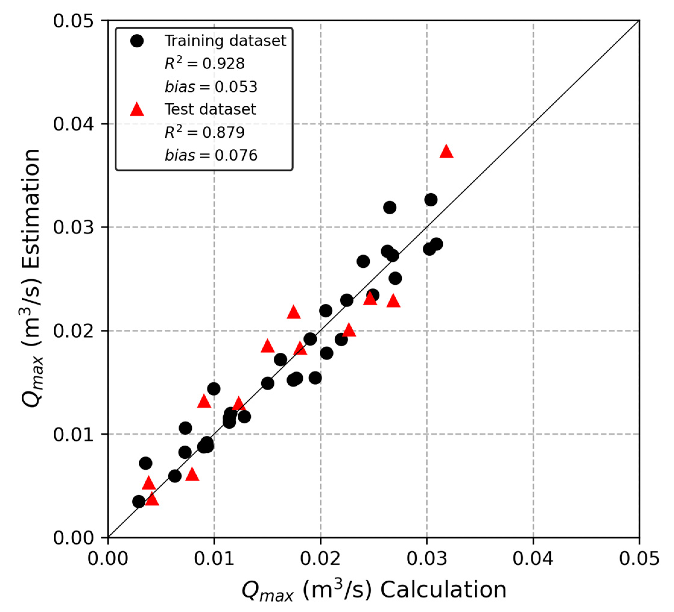
3.4. Maximum Instantaneous Overtopping Discharge

In extreme wave conditions, significant wave overtopping momentum can result from a large wave overtopping velocity and layer thickness, causing hazardous impacts over the breakwater crest. In this sub-section, the application of Equations (14) and (15) in the estimation of maximum instantaneous overtopping discharge is presented. Figure 11 illustrates the ratio of the occurrence of the maximum OFV (at $t_{\max u}$) and OLT (at $t_{max h_t}$) in the present study. From the figure, it can be observed that $t_{\max u}$ occurred slightly earlier than $t_{max h_t}$. The average of $t_{\max u}/t_{max h_t}$ is 0.914, and the gradient of the data in Figure 11 is $-$0.4. This indicates that the maximum OFV and OLT occurred almost at the same time. Based on this observation, we assume that the OFV and OLT occur at the same time by ignoring the time difference. Equation (16) is proposed to estimate the maximum instantaneous discharge ($Q_{max}$) as the product of the OFV and OLT:

$$Q_{max}=u{h}_t{c}_B$$

(16)

where $c_B$ is the cross-sectional width of breakwater crest.

The calculated and estimated $Q_{max}$ values are illustrated in Figure 12. The calculated $Q_{max}$ value was obtained from the experimental data of $u$ and $h_t$. In the estimated $Q_{max}$ value, Equations (14) and (15) were used to estimate $u$ and $h_t$. As shown in Figure 12, both the calculated and estimated $Q_{max}$ values demonstrate a good agreement, with $R^2=$ 0.928 and $bias=$ 0.053 for the training dataset, and $R^2=$ 0.879 and $bias=$ 0.076 for the testing dataset.

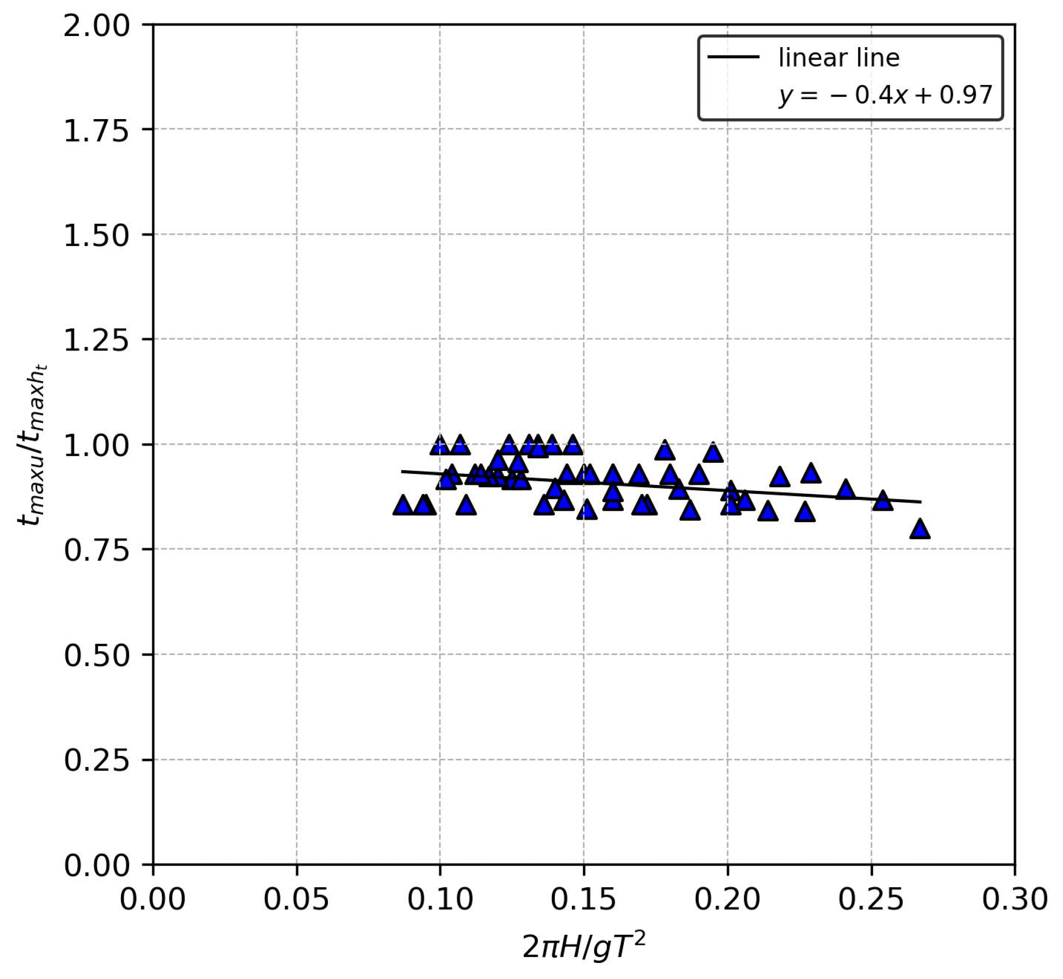
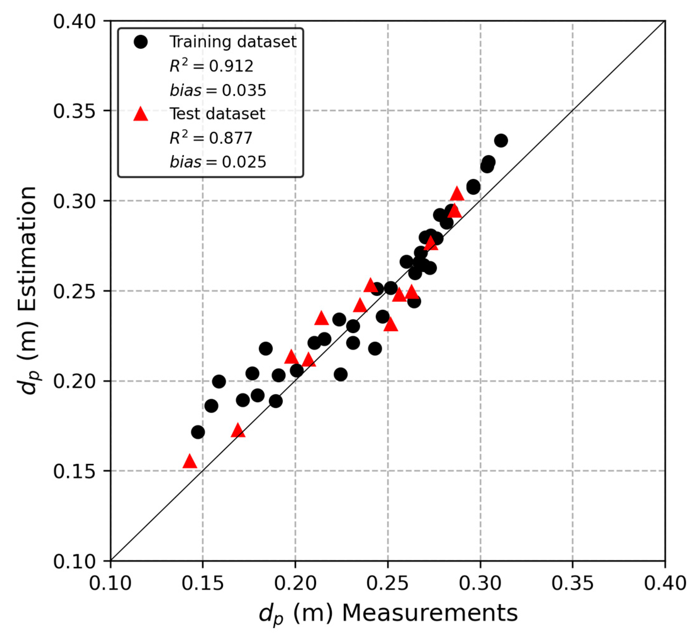
3.5. Plunging Distance

A study by Kudale and Kobayashi [36] revealed that the stability of the rear slope depends on the plunging location of the wave overtopping flow, especially in extreme waves, where overtopping into the rear side could result in a large momentum. Therefore, assessing the plunging location is one way to mitigate risks during the breakwater design process. The composite breakwater model used in this study did not have an armor unit on the rear side (see Figure 4), allowing for the wave overtopping flow to fall freely. This study used an imaging technique to measure the wave overtopping flow, facilitating the identification of the plunging location on the wave overtopping flow at the rear side of the breakwater. Thus, for a given wave condition, the estimation of the plunging location is possible.

As previously shown in Figure 5b, the plunging distance ($d_p$) is the horizontal distance from the rear side of the caisson into the midpoint of the wave overtopping jet tongue right before hitting the rear water surface. The $d_p$ value is determined by the OFV at the rear edge of the breakwater ($u$), the crest freeboard height ($R_c$), and the acceleration due to gravity ($g$):

$$d_p=\varphi \left(u,g,R_c\right)$$

(17)

The wave overtopping flow was assumed to undergo free fall towards the rear side, with negligible air friction. Therefore, $d_p$ can be calculated simply by multiplying $u$ and the free fall time, as shown in Equation (18).

$$d_p=u\sqrt{2R_c/g}$$

(18)

Figure 13 illustrates the comparison between the measured and estimated $d_p$ values for both the training and testing datasets. It is evident that the measured and estimated $d_p$ values show a strong agreement, with $R^2$ = 0.912 and $bias$ = 0.035 for the training dataset, and $R^2$ = 0.877 and $bias$ = 0.025 for the testing dataset.

4. Discussion

Estimating wave overtopping flow characteristics typically involves considering the incoming wave conditions at the structure’s toe and parameters related to the structure’s design. In this research, a straightforward empirical equation for both the OFV and the OLT at the rear edge of the composite breakwater was derived using a dimensional analysis. The OFV was normalized as $u/\sqrt{gH}$, and the OLT was normalized as $h_t/H$. The wave condition at the structure’s toe was represented by the wave steepness $2\pi H/{gT}^2$, and the structure’s geometry was represented by the relative crest freeboard $R_c/H$. These two dimensionless variables are commonly used in wave overtopping studies. The wave steepness, $2\pi H/{gT}^2$, influences the breaking process, while $R_c/H$ generally introduces hydraulic resistance to the overtopping flow.

The distribution of measured data for the OFV, as shown in Figure 8, exhibits increased scatter as $2\pi H/{gT}^2$ increases. A similar pattern is observed in the measurement data for OLT, as shown in Figure 10, albeit with even more scattered data. Steeper waves are associated with shorter wave periods and higher wave heights. Under these conditions, steeper waves tend to dissipate more energy when they interact with the structure’s front slope, as shown by $\xi <3.0$, resulting in greater data scatter. In Equations (14) and (15), we found that a power relationship best describes the relationship between $2\pi H/{gT}^2$ and $u/\sqrt{gH}$, as well as $h_t/H$. A negative value of the coefficient $n_u$ indicates an inverse power relationship, where $u/\sqrt{gH}$ and $h_t/H$ decrease as $2\pi H/{gT}^2$ increases. This inverse power relationship demonstrates that a higher wave steepness can lead to more significant energy dissipation. As waves interact with the structure, the collapsing water column transforms into turbulent flows, reducing the wave’s momentum and ability to overtop. On the other hand, $u/\sqrt{gH}$ and $h_t/H$ have a linear relationship with $R_c/H$, indicating that changes in the crest freeboard result in proportional changes in the wave overtopping flows. A larger crest freeboard may lead to greater energy dissipation of the incoming waves. As waves approach the breakwater crest subsequently, they are likely to encounter a change in flow regime and increased turbulence. This dissipation of wave energy contributes to a reduction in the intensity of the overtopping flow.

The results of this study indicate that both the wave steepness and crest freeboard offer more comprehensive descriptions of the OFV compared to using solely the relative crest freeboard, as shown in our previous study [30]. In our previous study, where we used only the relative crest freeboard, the $R^2$ value for OFV estimation was 0.730. In contrast, in this study, we observed an improvement with an $R^2=$ 0.955 in the training dataset and $R^2=$ 0.920 in the testing dataset. This improvement was likely due to the non-linear term in Equation (14), which enhanced the description of the complex interaction between waves and the structure. Moreover, employing the same set of dimensionless variables was also effective in describing the OLT.

A sensitivity analysis was performed to provide deeper insights into the impact of each dimensionless variable on wave overtopping flow, and the results are presented in Appendix B. Altering the empirical coefficients for $2\pi H/{gT}^2$ in Equations (14) and (15) resulted in an increase in $bias$. In these cases, the empirical equations tended to overestimate the OFV and OLT. Similarly, modifying the empirical coefficient for $R_c/H$ led to an increase in $bias$. Notably, the bias was negative, indicating that the empirical equations underestimated the OFV and OLT. The sensitivity analysis revealed that $2\pi H/{gT}^2$ significantly influences the OFV, while both $2\pi H/{gT}^2$ and $R_c/H$ influence the OLT. These results are consistent with the findings of Mares-Nassare et al. [20] and van Gent et al. [16], who also identified the influences of the wave steepness and crest freeboard on wave overtopping parameters.

Additional parameters of wave overtopping flow, $Q_{max}$ and $d_p$, were estimated using Equations (14) and (15). The estimated $Q_{max}$ using Equation (16) should be considered with caution as it may lead to overestimation. This is attributed to the nature of wave overtopping flow, characterized by a substantial presence of air bubbles. Consequently, the measurement of the OLT represents a combination of air and water. For precise estimations, the incorporation of a correction factor might be considered.

In EurOtop [5], $d_p$ is considered as one of the parameters of wave overtopping flow that is linked to the wave overtopping hazard, particularly in relation to the stability of the breakwater’s rear slope. This parameter is challenging to measure, and in most cases, an analysis is conducted by linking the rear slope stability with the wave conditions on the seaside. However, the use of a digital image technique in our experiment allowed us to directly measure this parameter. We employed an empirical equation, Equation (18), to estimate the plunging distance, while the OFV at the rear side of the breakwater was estimated using Equation (14). We obtained a good agreement between the measured and estimated $d_p$ values. It is worth noting that the empirical equation tends to overestimate the data in small and large value ranges, while underestimating it in the middle range. This discrepancy could be influenced by air entrainment and the characteristics of the shape of the falling fluid body, which were not considered in the estimation.

The set of equations (Equations (14)–(16) and (18)) were derived based on the conditions given in Table 4. It is important to note that regular waves were employed in this study. In real applications, however, waves are irregular. Regular waves establish a direct relationship between the wave conditions and wave overtopping parameters. To apply the present results to irregular wave conditions, it is essential to consider the corresponding irregular wave parameters ($H$ and $T$). An irregular wave height can be expressed through various parameters, including $H_s$, $H_{m0}$, $H_{1/x}$, and $H_{rms}$, while an irregular wave period can be represented by $T_s$, $T_p$, $T_{m-\mathrm{1,0}}$, and $T_m$ (refer to the Abbreviations section for explanations of each parameter). However, our study did not involve irregular waves, preventing a direct comparison. The study by Schüttrumpf and Oumeraci [13] showed that the same equations and empirical coefficients are applicable to estimate the wave run-up and overtopping parameters under both regular and irregular waves. Based on that study, we suggest the readers use $H_s$ and $T_m$ as the irregular wave parameters when applying the empirical equations in this study. To obtain the optimum estimation, we also recommend recalculating the empirical coefficients in Equations (14) and (15) for the given structure and wave conditions.

Here, we summarize the step-by-step process for the estimation of the OFV and OLT:

• Define the following irregular wave parameters for the design structure: the significant wave height ($H_s$), the averaged wave period ($T_m$), and the relative crest freeboard parameter ($R_c$).
• Calculate the wave steepness ($2\pi H/{gT}^2$) and the relative crest freeboard parameter ($R_c/H$).
• Compute the empirical parameters, $a_u$, $n_u$, and $b_u$, for Equation (14) and calculate the empirical parameters, $a_h$, $n_h$, and $b_h$, for Equation (15).
• Estimate the expected maximum OFV using Equation (14) and the maximum OLT using Equation (15).
• Plot the OFV and OLT for a given range of wave steepness values and relative crest freeboard.
• Utilize the range of the OFV and OLT for an early investigation of wave overtopping parameters based on the given wave and structure conditions.

The safety of the pedestrians on another type of structure (e.g., seawall) is also important. The set of equations proposed in this study might be applicable to other types of structures. As depicted in Figure 8 and Figure 10, selecting the appropriate empirical coefficient could provide a close estimation of real values. However, since the derived equations are obtained based on the test of tetrapod armored structures with a permeable core, the application of the present set of equations to other types of structures is uncertain. Further research encompassing irregular waves and a broader range of structural geometries will be conducted to better understand the impact of irregular waves on overtopping for practical coastal engineering applications.

5. Conclusions

Composite breakwater crests frequently serve as walkable areas, and ensuring pedestrian safety is a fundamental concern in breakwater design. Evaluating pedestrian safety relies heavily on wave overtopping parameters, specifically OFV and OLT. Nonetheless, existing studies have predominantly concentrated on OFV and OLT, concerning impermeable structures like sea dikes, with limited exploration in the context of permeable structures, such as composite breakwaters. To fill this research gap, our study delves into the investigation of the OFV and OLT on a composite breakwater through physical experiments.

The composite breakwater used in the study features a front slope with $V/H=1/1.5$ and a crest freeboard, $R_c=$ 0.12 m. A total of 55 regular wave conditions were employed to generate wave overtopping, and the BIV technique (bubble image velocimetry) was used to measure the wave overtopping parameters. Regular waves were used because they provide direct values for the OFV and OLT, corresponding to given wave conditions, such as the wave height and period. These values are crucial in the initial stages of designing specific structures under extreme wave conditions or assessing pedestrian safety on breakwater crests. In addition to the OFV and OLT, the parameter $d_p$, representing the plunging distance, was also obtained using digital imaging techniques. For the analysis, the experiment data were randomly split into training and testing datasets.

The proposed empirical equations for the OFV (Equation (14)) and OLT (Equation (15)), based on the dimensionless variables of the wave steepness ($2\pi H/{gT}^2$) and relative crest freeboard ($R_c/H$), demonstrate a strong agreement with the training and testing datasets. These results indicate the effectiveness of the proposed equations in estimating the OFV and OLT based on the wave steepness and relative crest freeboard. Furthermore, the sensitivity analysis reveals that $2\pi H/{gT}^2$ significantly influences the OFV, while both $2\pi H/{gT}^2$ and $R_c/H$ influence the OLT. This highlights the importance of considering these dimensionless variables in estimating wave overtopping parameters.

To illustrate the practicality of the empirical equations, we carried out an initial application. This involved estimating both the maximum instantaneous wave overtopping discharge ($Q_{max}$) and the plunging distance of the wave overtopping flow ($d_p$). $Q_{max}$ was estimated using Equation (16), and the comparison between the estimated and calculated $Q_{max}$ demonstrates good agreement. Similarly, the estimation of $d_p$ using Equation (18) exhibits good agreement with the experimental data. These results further support the effectiveness of the empirical equations in estimating wave overtopping parameters, allowing for the assessment of maximum instantaneous wave overtopping discharge and the plunging distance of the overtopping flow.

The outcomes of this research provide insights into the physical processes governing wave overtopping, serving as an initial exploration in the context of composite breakwater design. Moreover, through this study, the successful application of non-intrusive flow measurement techniques in wave overtopping has been demonstrated. While regular waves offer a controlled and systematic approach for studying specific wave characteristics, it is important to acknowledge that the results may differ from real-world scenarios where irregular waves are present. To apply the results of the present study, we suggest using $H_s$ and $T_m$ from irregular waves as the wave conditions input in Equations (14) and (15). An adjustment of the empirical coefficients is also needed to achieve an optimum outcome.

References

1. Bae, H.U.; Yun, K.M.; Yoon, J.Y.; Lim, N.H. Human Stability with Respect to Overtopping Flow on the Breakwater. Int. J. Appl. Eng. Res. 2016, 11, 111–119. [Google Scholar]
2. Gao, J.; Ma, X.; Dong, G.; Chen, H.; Liu, Q.; Zang, J. Investigation on the Effects of Bragg Reflection on Harbor Oscillations. Coast. Eng. 2021, 170, 103977. [Google Scholar] [CrossRef]
3. Gao, J.; Shi, H.; Zang, J.; Liu, Y. Mechanism Analysis on the Mitigation of Harbor Resonance by Periodic Undulating Topography. Ocean Eng. 2023, 281, 114923. [Google Scholar] [CrossRef]
4. Jeong, S.-H.; Heo, K.-Y.; Son, J.-H.; Jo, Y.-H.; Choi, J.-Y.; Kwon, J.-I. Characteristics of Swell-like Waves in the East Coast of Korea Using Atmospheric and Wave Hindcast Data. Atmosphere 2022, 13, 286. [Google Scholar] [CrossRef]
5. Van der Meer, J.W.; Allsop, N.W.H.; Bruce, T.; De Rouck, J.; Kortenhaus, A.; Pullen, T.; Schüttrumpf, H.; Troch, P.; Zanuttigh, B. EurOtop-Manual on Wave Overtopping of Sea Defences and Related Structures: An Overtopping Manual Largely Based on European Research, but for Worldwide Application; TU Delft: Delft, The Netherlands, 2018. [Google Scholar]
6. Franco, L.; de Gerloni, M.; van der Meer, J.W. Wave Overtopping on Vertical And Composite Breakwaters. In Coastal Engineering; Edge, B.L., Ed.; American Society of Civil Engineers: Kobe, Japan, 1994; pp. 1030–1045. [Google Scholar]
7. Cao, D.; Yuan, J.; Chen, H.; Zhao, K.; Liu, P.L.-F. Wave Overtopping Flow Striking a Human Body on the Crest of an Impermeable Sloped Seawall. Part I: Physical Modeling. Coast. Eng. 2021, 167, 103891. [Google Scholar] [CrossRef]
8. Cao, D.; Chen, H.; Yuan, J. Inline Force on Human Body Due to Non-Impulsive Wave Overtopping at a Vertical Seawall. Ocean Eng. 2021, 219, 108300. [Google Scholar] [CrossRef]
9. Abt, S.R.; Wittier, R.J.; Taylor, A.; Love, D.J. Human Stability in a High Flood Hazard Zone. J. Am. Water Resour. Assoc. 1989, 25, 881–890. [Google Scholar] [CrossRef]
10. Endoh, K.; Takahasi, S. Numerically Modeling Personnel Danger on a Promenade Breakwater Due to Overtopping Waves. In Coastal Engineering 1994; American Society of Civil Engineers: Reston, VA, USA, 1995; pp. 1016–1029. [Google Scholar]
11. Jonkman, S.N.; Penning-Rowsell, E. Human Instability in Flood Flows. JAWRA J. Am. Water Resour. Assoc. 2008, 44, 1208–1218. [Google Scholar] [CrossRef]
12. Sandoval, C.; Bruce, T. Wave Overtopping Hazard to Pedestrians: Video Evidence from Real Accidents. In Coasts, Marine Structures and Breakwaters 2017; ICE Publishing: London, UK, 2018; pp. 501–512. [Google Scholar]
13. Schüttrumpf, H.; Oumeraci, H. Layer Thicknesses and Velocities of Wave Overtopping Flow at Seadikes. Coast. Eng. 2005, 52, 473–495. [Google Scholar] [CrossRef]
14. Schüttrumpf, H.; van Gent, M.R.A. Wave Overtopping at Seadikes. In Coastal Structures 2003; American Society of Civil Engineers: Reston, VA, USA, 2003; pp. 431–443. [Google Scholar]
15. Van der Meer, J.W.; Hardeman, B.; Steendam, G.J.; Schuttrumpf, H.; Verheij, H. Flow Depths and Velocities at Crest and Landward Slope of a Dike, in Theory and with The Wave Overtopping Simulator. Coast. Eng. Proc. 2011, 1, 10. [Google Scholar] [CrossRef]
16. van Gent, M.R.A.; Wolters, G.; Capel, A. Wave Overtopping Discharges at Rubble Mound Breakwaters Including Effects of a Crest Wall and a Berm. Coast. Eng. 2022, 176, 104151. [Google Scholar] [CrossRef]
17. Mares-Nasarre, P.; Argente, G.; Gómez-Martín, M.E.; Medina, J.R. Overtopping Layer Thickness and Overtopping Flow Velocity on Mound Breakwaters. Coast. Eng. 2019, 154, 103561. [Google Scholar] [CrossRef]
18. Hughes, S.A.; Thornton, C.I.; Van der Meer, J.W.; Scholl, B.N. Improvements in Describing Wave Overtopping Processes. Coast. Eng. Proc. 2012, 1, 35. [Google Scholar] [CrossRef]
19. Mares-Nasarre, P.; Gómez-Martín, M.E.; Medina, J.R. Influence of Mild Bottom Slopes on the Overtopping Flow over Mound Breakwaters under Depth-Limited Breaking Wave Conditions. J. Mar. Sci. Eng. 2020, 8, 3. [Google Scholar] [CrossRef]
20. Mares-Nasarre, P.; Molines, J.; Gómez-Martín, M.E.; Medina, J.R. Explicit Neural Network-Derived Formula for Overtopping Flow on Mound Breakwaters in Depth-Limited Breaking Wave Conditions. Coast. Eng. 2021, 164, 103810. [Google Scholar] [CrossRef]
21. Nørgaard, J.Q.H.; Lykke Andersen, T.; Burcharth, H.F. Distribution of Individual Wave Overtopping Volumes in Shallow Water Wave Conditions. Coast. Eng. 2014, 83, 15–23. [Google Scholar] [CrossRef]
22. Bosman, G.; van der Meer, J.; Hoffmans, G.; Schüttrumpf, H.; Verhagen, H.J. Individual Overtopping Events at Dikes. Coast. Eng. 2009, 5, 2944–2956. [Google Scholar] [CrossRef]
23. Van Gent, M.R.A. Wave Overtopping Events at Dikes. In Coastal Engineering 2002; World Scientific: Singapore, 2002; pp. 2203–2215. ISBN 978-981-238-238-2. [Google Scholar]
24. Koosheh, A.; Etemad-Shahidi, A.; Cartwright, N.; Tomlinson, R.; van Gent, M.R.A. Individual Wave Overtopping at Coastal Structures: A Critical Review and the Existing Challenges. Appl. Ocean Res. 2021, 106, 102476. [Google Scholar] [CrossRef]
25. Ryu, Y.; Chang, K.-A.; Lim, H.-J. Use of Bubble Image Velocimetry for Measurement of Plunging Wave Impinging on Structure and Associated Greenwater. Meas. Sci. Technol. 2005, 16, 1945. [Google Scholar] [CrossRef]
26. Pedrozo-Acuña, A.; de Alegría-Arzaburu, A.R.; Torres-Freyermuth, A.; Mendoza, E.; Silva, R. Laboratory Investigation of Pressure Gradients Induced by Plunging Breakers. Coast. Eng. 2011, 58, 722–738. [Google Scholar] [CrossRef]
27. Lim, H.; Chang, K.; Huang, Z.; Na, B. Experimental Study on Plunging Breaking Waves in Deep Water. J. Geophys. Res. Oceans 2015, 120, 2007–2049. [Google Scholar] [CrossRef]
28. Ryu, Y.; Chang, K.-A.; Mercier, R. Runup and Green Water Velocities Due to Breaking Wave Impinging and Overtopping. Exp. Fluids 2007, 43, 555–567. [Google Scholar] [CrossRef]
29. Raby, A.; Jayaratne, R.; Bredmose, H.; Bullock, G. Individual Violent Wave-Overtopping Events: Behaviour and Estimation. J. Hydraul. Res. 2020, 58, 34–46. [Google Scholar] [CrossRef]
30. Adibhusana, M.N.; Lee, J.-I.; Ryu, Y. Wave Overtopping Plunging on the Rear Side of Composite Breakwater. J. Coast. Res. 2021, 114, 574–578. [Google Scholar] [CrossRef]
31. Adibhusana, M.N.; Lee, J.-I.; Kim, Y.-T.; Ryu, Y. Study of Overtopping Flow Velocity and Overtopping Layer Thickness on Composite Breakwater under Regular Wave. J. Mar. Sci. Eng. 2023, 11, 823. [Google Scholar] [CrossRef]
32. Bruce, T.; van der Meer, J.W.; Franco, L.; Pearson, J.M. Overtopping Performance of Different Armour Units for Rubble Mound Breakwaters. Coast. Eng. 2009, 56, 166–179. [Google Scholar] [CrossRef]
33. Schüttrumpf, H.; Möller, J.; Oumeraci, H. Overtopping Flow Parameters on The Inner Slope of Seadikes. In Coastal Engineering 2002; World Scientific Publishing Company: Singapore, 2002; pp. 2116–2127. [Google Scholar]
34. Molines, J.; Medina, J.R. Calibration of Overtopping Roughness Factors for Concrete Armor Units in Non-Breaking Conditions Using the CLASH Database. Coast. Eng. 2015, 96, 62–70. [Google Scholar] [CrossRef]
35. Goda, Y. Random Seas and Design of Maritime Structures; World Scientific Publishing Company: Singapore, 2010; Volume 33, ISBN 9813101024. [Google Scholar]
36. Kudale, M.D.; Kobayashi, N. Hydraulic Stability Analysis of Leeside Slopes of Overtopped Breakwaters. In Coastal Engineering 1996; American Society of Civil Engineers: New York, NY, USA, 1997; pp. 1721–1734. [Google Scholar]
Figure 2. Flow chart of the present study.
Water 15 04239 g002
Figure 3. Sketch of the two-dimensional wave flume used in this study.
Water 15 04239 g003
Figure 4. Dimensions of the composite breakwater used in this study. The dashed line shows the camera’s field of view (FOV).
Water 15 04239 g004
Figure 5. Velocity maps of the wave overtopping flow: (a) reached the rear edge of the breakwater; (b) plunged into the water surface on the rear side of the breakwater.
Water 15 04239 g005
Figure 6. Time series of u and h t at the rear edge of the breakwater. The red marker indicates the maximum u and h t .
Water 15 04239 g006
Figure 7. Scatter plot of wave overtopping flow velocity versus wave steepness and relative crest freeboard.
Water 15 04239 g007
Figure 8. The comparison between empirical equations (this study Equation (14), EurOtop [5], Mares-Nassare et al. [20], and Adibhusana et al. [31]) for OFV estimation with the training and testing datasets.
Water 15 04239 g008
Figure 9. Scatter plot of wave overtopping layer thickness versus wave steepness and relative crest freeboard.
Water 15 04239 g009
Figure 10. A comparison between empirical equations (this study Equation (15), EurOtop [5], Mares-Nassare et al. [20], and Adibhusana et al. [31]) for OLT estimation with the training and testing datasets.
Water 15 04239 g010
Figure 11. Dimensionless time occurrence of OFV and OLT.
Water 15 04239 g011
Figure 12. Comparison of the calculated and estimated Q m a x values in the training and testing datasets. The calculated Q m a x was obtained using the measured u and h t values, while the estimated Q m a x value was obtained by estimating u and h t using Equations (14) and (15), respectively.
Water 15 04239 g012
Figure 13. A comparison of the measured and estimated plunging distances ( d p ) using Equation (18) in both the training and testing datasets.
Water 15 04239 g013