Abstract
During the cofferdam construction of the toe reinforcement project at the Qiantang River Estuary, the scouring of the riverbed at the groin head often led to the collapse of geotube groins due to strong tidal currents. Based on field experience, employing a combination of clay and geotubes proved to be a more effective solution to this problem. This study adopted a flume model experiment to investigate the scouring and deposition around geotube groins and mixed clay–geotube groins. The results indicated that the influence of tidal surges on geomorphic changes surrounding the groins was more pronounced during spring tides than during neap tides. Under the same flow conditions, the scour depth at the head of the geotube groin was notably deeper than that of the mixed clay–geotube groin. Additionally, sediment silting behind the mixed clay–geotube groin was significantly greater than that behind the geotube groin. The clay component of the mixed clay–geotube groin served to mitigate the head scour, enhancing the overall structural stability to a certain extent. The geotube groin, with its surrounding scour pits expanding over time, experienced increasing tensile strain. This resulted in the rupture of the geotextile material, the loss of internal sand and, ultimately, groin collapse. It was found that mixed clay–geotube groins were better suited for cofferdam construction in strong tidal estuaries compared to geotube groin alternatives.
1. Introduction
The Qiantang River Estuary, spanning from the Fuchun River Power Station in Tonglu to the line connecting Luchao Port in Shanghai with Zhenhai in Ningbo, is a globally renowned strong tidal estuary, stretching approximately 290 km [1]. The north embankment of the Qiantang River is an essential barrier safeguarding the Hangjiahu Plain and the southern edges of Suzhou and Songjiang in Shanghai against typhoon storm surges. The Haining section of the Qiantang River’s northern embankment, measuring about 55.7 km, is composed of segments like the Yancang Embankment, the historical Qing Dynasty Embankment, and the Jianshan Embankment. Recent monitoring has revealed that parts of the sea embankment between Yangtian Temple and Tashan do not meet the original design standards for overall stability and scour protection. Under a 300-year event standard, 16.475 km of the embankment toe fails to meet the specified requirements [2]. To ensure flood and tide defense, there is an urgent need for a provisional cofferdam, facilitating reinforcement work for the embankment toe between Yangtian Temple and Tashan.
Given the intense tidal surges of this section of the Qiantang River, coupled with rapid flow velocities and significant river bed changes, constructing a cofferdam here is exceptionally challenging. Ensuring the temporary cofferdam’s stability during the 3–4-month construction period is paramount. Drawing from construction experience, the groins, on the one hand, act as flow deflectors, reducing the water current’s impact on the main cofferdam body and ensuring safety. On the other hand, they promote sediment deposition behind the groins, raising the riverbed to save construction costs, and can function as transverse cofferdams, enhancing construction efficiency. Thus, this project adopted a strategy of building vertical groins along the embankment, followed by the construction of the longitudinal cofferdam (as shown in Figure 1). Initially, geotube groins were used as transverse cofferdams. However, approximately 50–60 m offshore, significant scouring of the riverbed sand at the groin’s toe was observed. Progressive undercutting led to eccentric loading on the groin, causing local tensile deformation in the geotubes. When localized tensile forces surpassed the geotube’s tensile strength, it would be pulled to failure, resulting in a loss of fill material and the eventual collapse (as depicted in Figure 2), which incurred significant losses. Subsequently, an approach to integrating clay with geotube groins (referred to as mixed clay–geotube groins) was employed. The region near the embankment (within 50 m offshore) used geotube groins, while areas with faster water currents on the river side employed natural clay (as illustrated in Figure 3). The mixed clay–geotube groins were able to maintain their overall structural integrity without significant deformation during strong tidal surge periods, ensuring the smooth running of the project. Moreover, the sediment deposition efficiency behind the mixed clay–geotube groins was notably higher than that behind the geotube groins, offering convenience for subsequent longitudinal cofferdam construction.
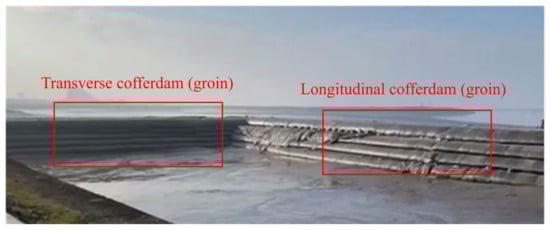
Figure 1.
Transverse cofferdam and longitudinal cofferdam.
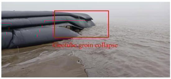
Figure 2.
Geotube groin collapse.
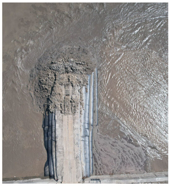
Figure 3.
Mixed clay–geotube groin.
The groin is one kind of spur dike that is often used in temporary water-related projects. Comprehensive studies on scouring and protection around groins are vital in actual engineering scenarios [3]. Considerable progress has been made in understanding the scouring and deposition around groins [4,5,6,7,8,9,10]. However, the fluid dynamics around these structures becomes intricate in estuaries with strong tidal actions, and studies in this area remain insufficient. In the context of field measurements, Zhao et al. [11,12,13] carried out observations and comparative analyses of pile-supported groins intended for dike protection. Field measurements of scour holes around the groins and observations of their influence on the elevation and tidal bores of nearby tidal flats revealed that, compared to traditional rock-filled groins, pile-supported groins demonstrated less local scouring around the structure, better stability, and notable effectiveness in moderating tidal bore velocities. Experimentally, Qian et al. [14] combined holistic physical modeling to simulate the behavior of groins in bends and flume modeling to study groins in straight sections, investigating differences in localized scouring under strong tidal action. Their results indicated that groins located on bends experienced deeper local scour holes than those on straight sections when subjected to strong tidal action. Zhang et al. [15] took the spur dike in the Qiantang River Estuary’s Jianshan section as a prototype and conducted flume experiments on submerged groin scouring induced by tidal bores. The results showed that the scour depth was directly proportional to the relative current intensity and the dike height, but inversely proportional to the water depth before the bore. Pan and Li [16] used flume models to investigate the hydraulic structures, scour hole morphology, and depth around the widely used sheet-pile groins in the Qiantang River Estuary. They obtained the fitted maximum scour depth calculation formulae at the groin head and the upstream side of a groin using the least squares method. Numerically, conventional models struggled to accurately simulate the water process under the influence of tidal bores, due to the discontinuity of physical quantities before and after the tidal bores. Initial efforts focused on exploring tidal bores’ propagation [17,18,19,20], followed by studies on sediment transport under the influence of groins [21,22,23,24,25,26]. However, most of these studies centered around permanent groins (e.g., rock-filled dikes, sheet-pile groins), with limited investigations of the often-used geotube groins in temporary water-related projects, and those available predominantly discussed their stability [27,28]. Research on scour and deposition around geotube groins, especially under tidal environments, is notably lacking. Additionally, studies on the innovative mixed clay–geotube groins, deduced from the latest engineering experiences, are virtually nonexistent.
Based on the embankment engineering project on the north bank of the Qiantang River, from Yangtian Temple to Tashan (specifically focusing on the toe of the dike), this study addresses the different performances of geotube groins and mixed clay–geotube groins (i.e., the instability and potential collapse of geotube groins and the relatively stable mixed clay–geotube groins under intense water flow). The remainder of this paper is structured as follows: Section 2 articulates the materials and methods adopted in this study, including the experimental setup and measurement equipment, the determination of the scale ratio, the selection of the model sediment, and the experimental design. Section 3 provides a detailed analysis of the experimental results. Section 4 discusses the potential reasons for the experimental results. Finally, conclusions and prospects for future works are presented in Section 5.
2. Materials and Methods
2.1. Experimental Setup and Measurement Equipment
The physical model experimentation was conducted in a multifunctional experimental flume with dimensions of 30 m in length, 10 m in width, and 1 m in height (as depicted in Figure 4). The flume featured a flat, ungraded bottom surface along its entire length. The experimental water supply was facilitated through a closed-loop water supply system, with a maximum flow rate of 400 L/s achievable through precision control by an intelligent flow control system. In the outflow section of the flume, adjustable sluice gates and baffles were installed to regulate both the outflow rate and the water depth. The primary flume was characterized by its flat-bottomed profile, rendering it unsuitable for dynamic bed experiments. To overcome this limitation, a custom-built, portable sediment flume was constructed within the experimental flume. This sediment flume measured 4 m in length, 3 m in width, and 0.2 m in depth. Transition sections measuring 4.8 m and 3.6 m in length, respectively, were positioned at the inlet and outlet ends of the sediment flume to ensure a relatively stable flow profile as the water entered the dynamic bed testing segment.
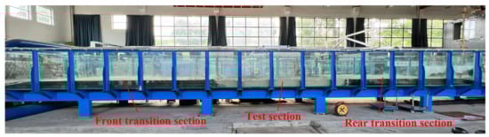
Figure 4.
Experimental flume and sediment flume.
Utilizing our independently developed high-precision automated topographic instrument for sediment–water physical experiments (as depicted in Figure 5), we monitored changes in the terrain. This instrument is capable of stable operation, facilitating measurements of the experimental terrain in varying sediment–water environments. It is equipped with a high-precision probe that records the descent height as soon as the probe makes contact with the riverbed after being lowered from its initial height. For a given point, the difference between the descent heights recorded by the topographic instrument in its initial and final terrain states represents the terrain change at that point.
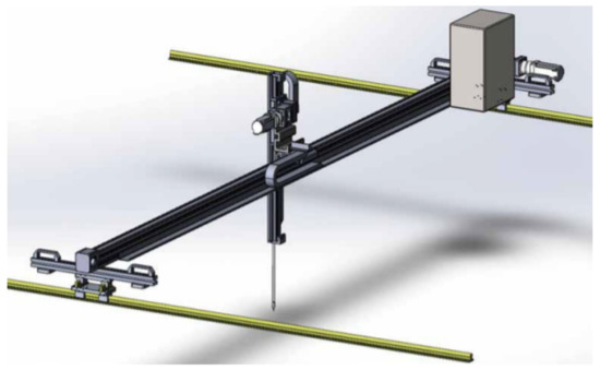
Figure 5.
High-precision topographic instrument.
2.2. Similarity Conditions and Scale Ratio
The physical experiment primarily focused on the local scour and sedimentation variations around the groins, characterized by significant three-dimensionality. As the variations in scour and sedimentation at the Qiantang River Estuary are predominantly influenced by the suspended sediment transport dynamics [29,30], the experimental design adhered to the principles of the normal sediment transport bed model. Complying with the specifications outlined in hydraulic model testing standards [31], it needed to simultaneously satisfy conditions of hydraulic similarity and sediment transport similarity. Additionally, to ensure minimal perturbation of the flow patterns around the model groin by the opposite flume sidewall, the length of the model groin should not exceed approximately one-third of the flume’s width according to numerical simulations. The selected experimental scale ratios are presented in Table 1.

Table 1.
Scale ratio determination.
2.3. Selection of Model Sediment
This model adhered to the principles of a normal sediment transport bed model for suspended sediment, with the selection of the model sediments primarily governed by considerations of sediment transport similarity and incipient motion similarity. In the construction zone of the groin, the average water depth typically fell within the range of 2 to 5 m, and the median particle size d50 of the riverbed sediment was within the range of 0.03 mm to 0.06 mm. Within this specified range of water depth and median particle size, the selection of the model sediments aligned with Zhang Ruijin’s formulae for incipient flow velocity (Equation (1)) and settling velocity (Equation (2)).
where Ue refers to the initiation velocity of the sediment, h refers to the depth of the water in the construction area, d refers to the median particle size of the sediment, and ρs and ρ refer to the density of the sediment and water, respectively.
where w refers to the settling velocity of the sediment, v refers to the flow velocity of the water, and g stands for the gravitational acceleration.
It could be determined that the average incipient flow velocity for sediment transport in this region fell within the range of 0.47 m/s to 0.71 m/s, while the settling velocity ranged from 0.06 cm/s to 0.18 cm/s. Based on the calculations of prototype sediment settling, incipient flow velocity, and scale analysis, the model sediment should exhibit incipient flow velocities ranging from 5.2 cm/s to 8.3 cm/s and settling velocities between 0.008 cm/s and 0.03 cm/s. Following the comparative analysis of various model sediments’ incipient flow velocities by experimentation, a model sediment consisting of wood powder (Ziyang Wood Powder Factory, Ziyang, Shandong, China) with a density of 1.2 t/m3 and a median particle size of 0.1 mm was selected for the dynamic bed experiments. The model sediment exhibited an incipient flow velocity of 6.5 cm/s and a settling velocity of 0.028 cm/s.
2.4. Experimental Design
2.4.1. Groin Models
To investigate and compare the bed changes in the surrounding topography induced by both geotube groins and mixed clay–geotube groins under varying flow conditions, it was necessary to make the groin models prior to the flume experiments. These models were designed based on the dimensions of the field prototype groins (with a length of 48 m, a base width of 36 m, a top width of 12 m, and a height of 12 m) and the prescribed geometric scaling ratios. This ensured that the constructed groin models maintained the same overall dimensions, with respective lengths, widths, and heights of 60 cm, 45 cm, and 15 cm. For the model of the geotube groin, a prototype geotextile material from the construction site was used for stitching. The geotubes were internally filled with riverbed sediment. The construction comprised three segments with dimensions of 60 cm × 45 cm × 5 cm, 60 cm × 30 cm × 5 cm, and 60 cm × 15 cm × 5 cm, respectively. These were stacked in descending order by size from bottom to top, as illustrated in Figure 6. In the case of the mixed clay–geotube groin model, it included both a section with geotubes and a section with clay material. The three geotube models had dimensions of 47 cm in length, 45 cm in width, and 5 cm in height; 47 cm in length, 30 cm in width, and 5 cm in height; and 47 cm in length, 15 cm in width, and 5 cm in height, respectively. The stacking configuration of these models was consistent with that of the geotube groin. Additionally, a layer of clay was applied at the head of the geotube models, closely adhering to the groin head. This clay layer had a height of 15 cm and extended outward by 13 cm, as depicted in Figure 7. Subsequently, the fabricated models were individually placed in flumes filled with saturated model sediment for experimental testing.
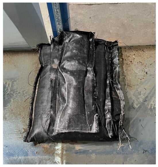
Figure 6.
Geotube groin model (model dimensions: length 60 cm, width 45 cm, height 15 cm).
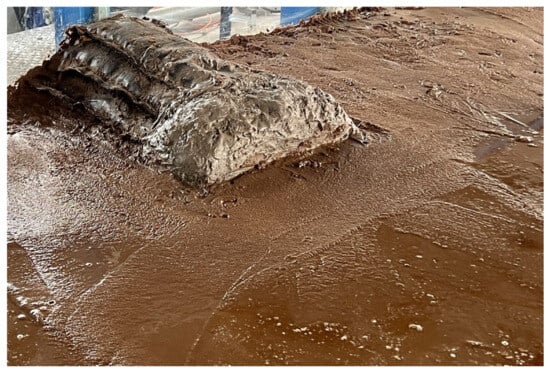
Figure 7.
Mixed clay–geotube groin model (model dimensions: length 60 cm, width 45 cm, height 15 cm; the geotube part: 47 cm long, 45 cm wide, and 15 cm high; the clay part: 13 cm long, 45 cm wide, and 15 cm high).
2.4.2. Measurement Point Configuration
Topographical measurements were systematically arranged across 37 longitudinal monitoring sections oriented perpendicular to the direction of the water flow. These sections were designated as sections 1-1 to 37-37, as illustrated in Figure 8. Upstream of the model groin, 10 longitudinal sections (Sections 1 to 10) were established, with intersectional spacings of 15, 10, 5, 5, 5, 5, 5, 2, 2, and 2 cm, respectively. Each of these longitudinal sections consisted of 15 points spaced 10 cm apart. At the groin head, 10 additional longitudinal sections (Sections 11 to 20) were set up, with 5 cm of spacing between adjacent sections, and each section contained 18 points with 5 cm intervals between points. Downstream of the model groin, there were 17 longitudinal sections (Sections 21 to 37), with respective intersectional spacings of 2, 2, 2, 5, 5, 5, 5, 5, 5, 10, 10, 10, 10, 10, 15, 15, and 20 cm. Each of these sections incorporated 15 points, with a spacing of 10 cm between the individual points.

Figure 8.
Measurement point distribution map (overall dimensions of the groin model shown as the black box: length 60 cm, width 45 cm, height 15 cm).
2.4.3. Experimental Conditions
The primary construction phase of the on-site engineering project spanned from October to May of the following year. This study focuses on the month of April as a representative case, examining the morphological changes due to sediment deposition and erosion around two types of groins under both spring and neap tidal flow conditions. A summary of the experimental conditions is presented in Table 2.
Table 2.
Summary table of experimental conditions.
Based on tidal data obtained from the Yanguan tide gauge station, representative hydrodynamic conditions were selected from two distinct days in April: one with the maximum tidal range (1 April, representing spring tide), and the other with the minimum tidal range (7 April, representing neap tide). Due to the inherently unsteady nature of the tidal cycle, the experimental approach utilized the concept of ‘quasi-steady flows’. In this method, a complete unsteady inflow and sediment transport process was approximated by several stepped steady processes. Consequently, for a complete tidal cycle, three periods were identified, and the flow conditions were graded based on the extent of the variations in water level and flow velocity in each period. These periods were the pre-flood period (where water levels rose gradually, divided into one grade), the rapid high-tide period (featuring significant changes in water level and flow velocity, divided into two grades), and the slack-water period (with minimal changes in water level, divided into one grade).
According to the data for water level and flow velocity provided by the Yanguan tide gauge station, the averaged water level divisions for neap and spring tides are illustrated in Figure 9 and Figure 10, respectively. Using the scale relationships established in Table 1, the variables are listed in Table 3 and Table 4, where V is the averaged flow velocity, H is the averaged water level, and variables of the prototype and the model are denoted by the subscripts p and m, respectively. Q is the pump discharge, and T is the scaled time for each period in the flume.
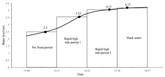
Figure 9.
Elevation gradation during the neap tide inflow period.
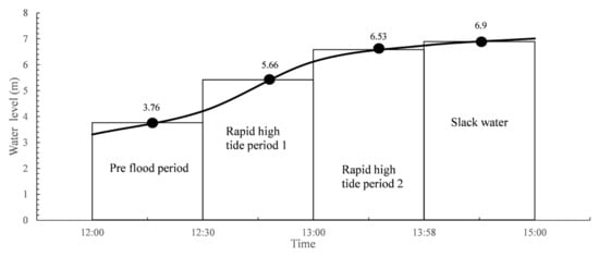
Figure 10.
Elevation gradation during the spring tide inflow period.
Table 3.
Parameters for each classification in the neap tide experiment.
Table 4.
Parameters for each classification in the spring tide experiment.
3. Results
3.1. Experimental Condition 1: Neap Tide Inflow
Under the inflow conditions of the neap tide, the initial and final topographies of both types of groins can be seen in Figure 11, where GG signifies the geotube groin, while MGG denotes the mixed clay–geotube groin.
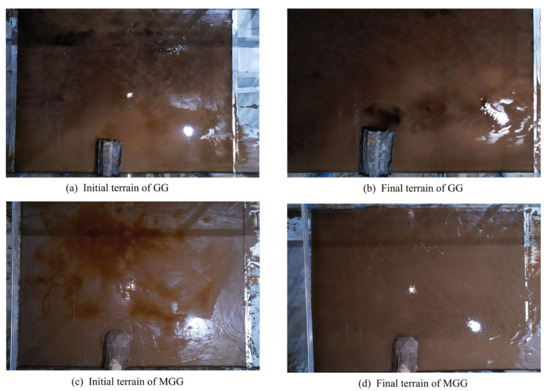
Figure 11.
Topographical changes around both types of groins under neap tide inflow conditions.
According to the topographic variations measured by the topographic instrument, the final contour lines of sedimentation and erosion for both types of groins were as illustrated in Figure 12, with both the horizontal and vertical axes scaled in mm. The model groins were positioned within the flume at coordinates ranging from 560 mm to 1010 mm on the x-axis and from 0 mm to 600 mm on the y-axis. The x-axis represents the longitudinal direction along the flume, while the y-axis represents the direction perpendicular to the flume.
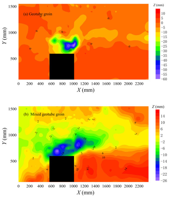
Figure 12.
Contour maps of sedimentation and erosion for two different groin materials during the neap tide inflow.
By synthesizing the overall topographic contour maps with high-resolution experimental images, it was evident that under conditions of neap tide inflow, the downstream terrain of both types of groins exhibited an increase in elevation. This observation corroborated that both groins were effective in promoting sedimentation in their respective downstream zones.
To offer a more detailed assessment of the extent of sediment accumulation behind the groins, elevational profiles from three selected downstream longitudinal section measurement points were analyzed, revealing the longitudinal variations, as shown in Figure 13. The distances from CS 22, CS 28, and CS 34 to the backwater side of the groin (CS 20) were 4 cm, 31 cm, and 86 cm, respectively. An elevation of 0 refers to the relative initial topography. An elevation greater than 0 indicates sedimentation, while elevation below 0 means bed erosion. In the downstream zone of the model groins located within approximately 600 mm from the shore, the elevation increase in the topography was more pronounced for the three longitudinal sections downstream of the mixed clay–geotube groin as compared to their counterparts downstream of the geotube groin. The relative sediment accretion exceeded 10 mm for the mixed clay–geotube groin, while it remained below 5 mm for the geotube groin. It was noted that areas in closer proximity to the mixed clay–geotube groin exhibited a higher degree of sedimentation. This was attributed to the partial dispersal of clay from the head of the mixed clay–geotube groin during erosive processes, which was then transported downstream and accumulated.
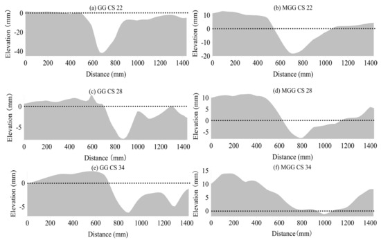
Figure 13.
Elevation change profile of the longitudinal section behind the groins.
In regions situated at a distance greater than 600 mm from the shore, the riverbeds surrounding both types of groins generally exhibited erosive tendencies, with the extent of erosion intensifying as the proximity to the groins increased. For any given longitudinal section, the erosion depth adjacent to the geotube groin was notably greater than that near the mixed clay–geotube groin. For instance, at section CS 22, the maximum erosion depths for both groins were located approximately 700 mm from the flume’s sidewall. The geotube groin exhibited an erosion depth of 40 mm, whereas the mixed clay–geotube groin showed a comparatively shallower depth of 20 mm. When comparing the topographic contour maps (as shown in Figure 12), the scour holes around the geotube groin were, on the whole, deeper than those around the mixed clay–geotube groin. The deepest erosion near the head of the geotube groin reached up to 60 mm, while that for the mixed clay–geotube groin was limited to 25 mm.
To further explore the erosional patterns at the heads of the two different groins, cross-sectional variations at distances of 5 cm (Y = 650 mm), 15 cm (Y = 750 mm), and 25 cm (Y = 850 mm) from the groin head were plotted. It can be seen in Figure 14 that the scour depth at the head of the geotube groin exceeded that of the mixed clay–geotube groin at the same cross-section. Specifically, the maximum scour depth observed for the geotube groin reached up to 60 mm, whereas it was limited to 20 mm for the mixed clay–geotube groin. However, the spatial extent of the scour pit associated with the mixed clay–geotube groin was broader than that associated with the geotube groin. The scour dimensions for the geotube groin spanned a range of 400 mm to 1200 mm, compared to 300 mm to 1400 mm for the mixed clay–geotube groin. In summary, during the period of neap tide inflow, the geotube groin exhibited greater scour depths, but within a narrower range, whereas the mixed clay–geotube groin manifested lower scour depths, but over a more expansive spatial domain.
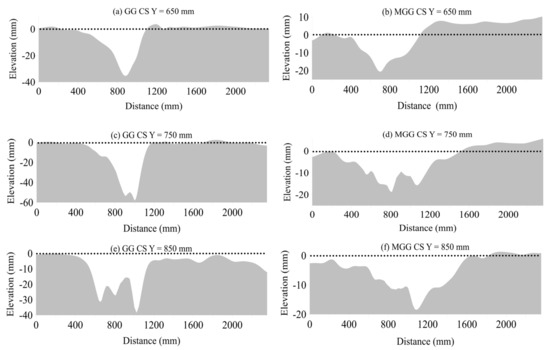
Figure 14.
Topographic elevation variation diagrams of cross-sections at various distances from the groin.
3.2. Experimental Condition 2: Spring Tide Inflow
Under the inflow conditions of the spring tide, the initial and final topographies of both types of groins can be seen in Figure 15.
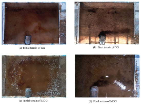
Figure 15.
Topographical changes around both types of groins under spring tide inflow conditions.
According to the topographic variations measured by the topographic instrument, the final contour lines of sedimentation and erosion for both types of groin were as illustrated in Figure 16. Both the x- and y-axes are represented in mm, and the location of the model groins in the flume correspond to conditions during the neap tide phase.
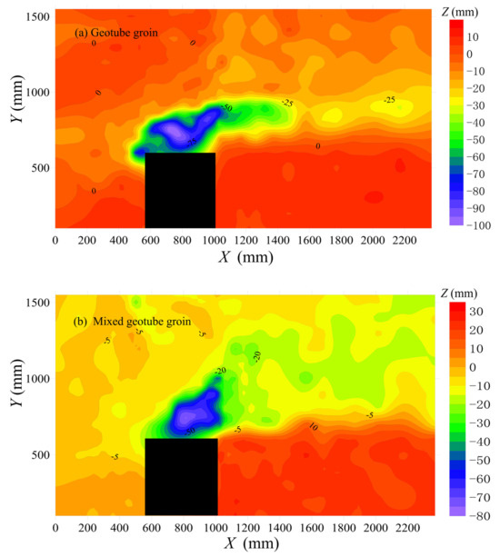
Figure 16.
Contour maps of sedimentation and erosion for two different groin materials during the spring tide inflow.
By comparing the overall contour lines of both groins, it can be observed that after the passage of the spring tide inflow, the post-groin topography of the geotube groin showed relative sedimentation between 5 mm and 10 mm (as shown in Figure 16a), while the sedimentation behind the mixed clay–geotube groin was between 20 mm and 30 mm (Figure 16b). This indicates that both types of groins enhanced sediment deposition in the downstream region, with the mixed clay–geotube groin demonstrating superior siltation promotion compared to the geotube groin. When compared with the neap tide inflow conditions, where the geotube groin had a relative sedimentation thickness of less than 5 mm (Figure 12a) and the mixed clay–geotube groin was between 10 mm and 15 mm (Figure 12b), it was evident that the spring tide inflow had a more pronounced effect on the post-groin topographic changes than the neap tide for both groins.
To offer a more detailed assessment of the extent of sediment accumulation behind the groins, elevational profiles from three selected downstream longitudinal section measurement points were analyzed, revealing the following longitudinal variations:
From Figure 17, it was evident that during the high tide of the spring tide, within the area behind the model groins (within 600 mm from the shoreline), the change in elevation across the three cross-sections behind the mixed clay–geotube groin was more pronounced compared to the corresponding positions behind the geotube groin. Relative to the conditions during the neap tide inflow, there was greater sediment accretion behind the mixed clay–geotube groin during the spring flood tide, with siltation approximately 20 mm thick, while the increase in sediment accretion behind the geotube groin during the spring tide inflow was rather modest compared to the neap tide conditions.
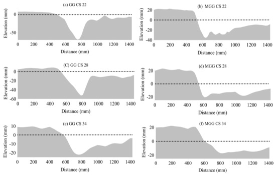
Figure 17.
Elevation change profile of the longitudinal section behind the groins.
Additionally, to further explore the erosional patterns at the heads of the two different groins, cross-sectional variations at distances of 5 cm (Y = 650 mm), 15 cm (Y = 750 mm), and 25 cm (Y = 850 mm) from the groin head were plotted, as shown in Figure 18. The geotube groin showed a greater scour depth at the groin head than the mixed clay–geotube groin. The maximum scour depth for the geotube groin reached up to 100 mm, while the mixed clay–geotube groin recorded a maximum scour depth of only 60 mm. It can be inferred that the geotube groin was more susceptible to scouring at the head compared to the mixed clay–geotube groin.
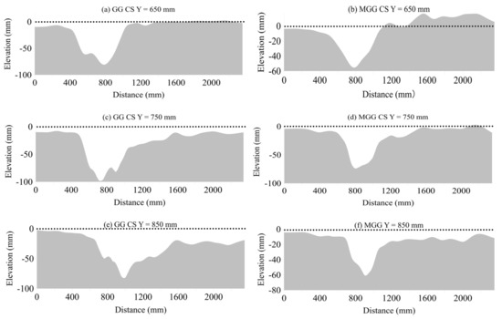
Figure 18.
Topographic elevation variation diagrams of cross-sections at various distances from the groins.
During the spring tide period, the scour pit depth for the geotube groin ranged from 0 to 100 mm, as depicted in Figure 18a,c,e. Conversely, the mixed clay–geotube groin’s scour pit depth ranged between 0 and 60 mm during the same phase, as shown in Figure 18b,d,f. The geotube groin’s head was found to experience more severe scouring than that of the mixed clay–geotube groin. Relative to the conditions during the neap tide, the geotube groin exhibited scour pit depth ranges of 0–40 mm (see Figure 14a,c,e), while the mixed clay–geotube groin showed ranges of 0–20 mm (as shown in Figure 14b,d,f). After the spring tide phase, the scour pit depths at the heads of both groins expanded by 1–2 times compared to those during the neap tide. This indicates that the spring tide exerted a more significant influence on the scour pits at the groin heads than the neap tide.
4. Discussion
By comparing the topographical changes around the model groins under different experimental conditions, it became evident that the spring tide exerted a more significant influence on the surrounding morphology than the neap tide. This was predominantly manifested in deeper scouring pits at the groin heads, wider affected areas, and increased sediment deposition downstream of the groins. During the spring tide, the increased flow velocity could mobilize more bed sediments into the flow, resulting in a higher sediment concentration within the water column. As the sediments were transported downstream of the groins, the flow velocity diminished, and more sediments settled, leading to morphological sediment deposition.
By comparing the morphological changes downstream of groins made of different materials under the same flow conditions, we found that sediment deposition was more pronounced behind mixed clay–geotube groin. This was attributed to the faster flow velocities during spring tide, where a portion of the clay within the mixed clay–geotube groin’s structure was eroded and dispersed by the water flow. Subsequently, the eroded material settled in areas with slower velocities downstream of the groin.
Figure 19 illustrates the phenomenon of head collapse in the geotube groin under the conditions of a spring tide. The geotube groin behaved approximately as a rigid body, with its base in direct contact with the original riverbed of sandy soil. Under prolonged, intense, unsteady flow, the bed sediment at the base of the geotube groin’s head was progressively eroded, forming a scour hole. This resulted in an eccentric load on the groin, causing localized tensile deformation of the geotextile material. In actual engineering scenarios, when the localized tensile force exerted on the geotube exceeded its tensile strength, the geotextile material was pulled into failure, leading to sand leakage, and the groin ultimately collapsed, as shown in Figure 2.
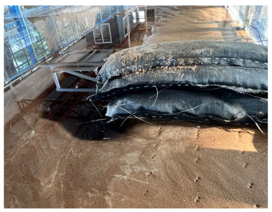
Figure 19.
Localized scour pit at the head of the geotube groin following the spring tide surge.
For the mixed clay–geotube groin, its head clay exhibited some erodibility. Our experimental findings indicated that under hydrodynamic forces, a portion of the clay from the mixed clay–geotube groin’s head was eroded and fell into the scour pit, which filled the pit to a certain extent, as demonstrated in Figure 20a. Unlike the geotube groin, the clay component of the mixed clay–geotube groin exhibited some flexibility. When a scour pit formed at its head, the clay underwent deformation and fitted the edges of the pit, preventing its extension beneath the main groin structure, as seen in Figure 20b. This could reduce the eccentric load on the groin, enhancing its overall stability. Meanwhile, some of the clay carried by the flow would fill the gap between the groin and the riverbed, adhering the bottom geotube layer to the riverbed and further bolstering the groin’s stability, as depicted in Figure 21.
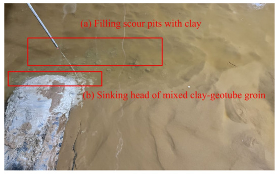
Figure 20.
Scour pit at the head of the mixed clay–geotube groin.
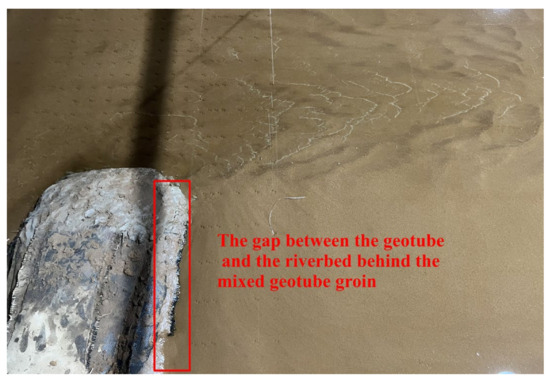
Figure 21.
Partial diagram of the contact between the geotube behind the mixed clay–geotube groin and the riverbed.
5. Conclusions
In the cofferdam construction process for the embankment toe reinforcement project at the Qiantang River Estuary, geotube groins often encountered problems of embankment head erosion, leading to the tearing of the geotextile material of geotube groins, the subsequent loss of infilled material and, finally, collapse. This significantly hindered the progress of the project. Drawing on engineering experience, adopting mixed clay–geotube groins could effectively address this issue. To provide theoretical support for this construction approach, we conducted flume model tests to study the sediment dynamics around groins of both material types under various flow conditions. The conclusions are as follows:
(1) In comparative terms, the morphological impacts on the surrounding terrain of the groins were more pronounced under conditions of spring tide inflow than under neap tide inflow conditions. Furthermore, under the same flow conditions, the scour pits at the heads of the geotube groin were conspicuously deeper than those formed around the mixed clay–geotube groin.
(2) From the perspective of sediment accretion effects behind the groins, both groins exhibited the capability to promote sediment deposition. Under two different flow conditions, the velocity of the water decreased in the region downstream of the groins, resulting in the settlement of suspended sediment, and thereby elevating the downstream terrain. It was noteworthy that during periods of spring tide, the increased flow velocity mobilized a greater quantity of bed sediment into the water column. As the flow decelerated downstream of the groins, a more substantial sediment deposition was observed. Under the same flow conditions, the mixed clay–geotube groin demonstrated a higher propensity for sediment accumulation in its downstream regions than the geotube groin. This was attributed to the fact that some of the clay within the structure of the mixed clay–geotube groin was eroded and transported downstream by the flowing water, contributing to enhanced sedimentation rates behind the groin.
(3) From the perspective of the groin stability, clay possesses certain erosive characteristics that have a unique interaction with the hydraulic environment. Under sustained water flow, some of the clay at the head of the mixed clay–geotube groin was scoured and displaced into existing scour pits, effectively serving a role in the infill and attenuation of these erosive features. Additionally, due to the inherent plasticity of clay, it had the ability to adapt its shape to conform to the contours of the scour pits, thereby bolstering the overall stability of the groin structure to a significant extent. Conversely, the geotube groin exhibited less favorable stability characteristics. Scour pits that formed at the groin head induced eccentric loading conditions, leading to deformation of the geotextile material. Once this deformation reached a critical threshold, the geotextile material experienced structural failure, causing the contained sand to leak and eventually resulting in groin collapse.
These findings highlight the benefits of mixed clay–geotube groins for their potential to enhance structural integrity and resilience against erosive forces in cofferdam construction at the Qiantang River Estuary, offering scientific support for the applicability of mixed clay–geotube groins in tidal areas.
However, it should be noted that due to the limited experimental conditions and test duration, the above conclusions were drawn under specific flow conditions, so there are certain limitations. In the future, tests under more conditions will be needed, such as setting various flow conditions, and adjusting the length and angle of the groins. Meanwhile, the durability, maintenance costs, and environmental compatibility of synthetic materials should also be investigated to protect natural water against the dispersion of artificial materials due to failures.
Author Contributions
Conceptualization, X.T. and C.X.; methodology, J.X.; validation, K.F.; formal analysis, J.X.; investigation, J.L.; resources, X.T.; writing—original draft preparation, J.X. and C.X.; writing—review and editing, J.X. and C.X.; visualization, H.G.; supervision, J.L. and C.X.; project administration, X.T. and K.F.; funding acquisition, X.P. All authors have read and agreed to the published version of the manuscript.
Funding
This research was funded by the National Natural Science Foundation of China (No. 12002310), Natural Science Foundation of Zhejiang Province (No. LZJWZ23E090010), and Science and Technology Projects of POWER CHINA HUADONG Engineering Co. Ltd. (No. KY2022-JG-03-02).
Data Availability Statement
The data presented in this study are available upon request from the corresponding author.
Acknowledgments
We would like to thank the Key Laboratory of Ocean Space Resource Management Technology at Zhejiang University of Water Resources and Electric Power for providing the experimental site. We also wish to thank the potential reviewers very much for their valuable comments and suggestions.
Conflicts of Interest
The authors declare no conflict of interest.
References
- Pan, C.; Wang, Q.; Pan, D.; Hu, C. Characteristics of river discharge and its indirect effect on the tidal bore in the Qiantang River, China. Int. J. Sediment Res. 2023, 38, 253–264. [Google Scholar] [CrossRef]
- Pan, C. Special Research Report on Scouring at the Foot of the Ancient Sea Dyke on the North Shore of Qiantang River; Zhejiang Provincial Institute of Water Resources and Estuary: Hangzhou, China, 2019. (In Chinese) [Google Scholar]
- Wang, D. Study of local scour around submerged spur-dikes. Adv. Hydrodyn. 1988, 3, 60–69. (In Chinese) [Google Scholar]
- Xu, H.; Li, Y.; Zhao, Z.; Wang, X.; Zhang, F. Experimental study on the local scour of submerged spur dike heads under the protection of soft mattress in plain sand-bed rivers. Water 2023, 15, 413. [Google Scholar] [CrossRef]
- Aung, H.; Onorati, B.; Oliveto, G.; Yu, G. Riverbed morphologies induced by local scour processes at single spur dike and spur dikes in Cascade. Water 2023, 15, 1746. [Google Scholar] [CrossRef]
- Zhang, L.; Wang, P.; Yang, W.; Zuo, W.; Gu, X.; Yang, X. Geometric characteristics of spur dike scour under clear-water scour conditions. Water 2018, 10, 680. [Google Scholar] [CrossRef]
- Han, X.; Lin, P.; Gary, P. Influence of layout angles on river flow and local scour in grouped spur dikes field. J. Hydrol. 2022, 614, 128502. [Google Scholar] [CrossRef]
- Reza, F.; Mahmood, S.K.; Mehdi, G.; Giuseppe, O. Temporal scour variations at permeable and angled spur dikes under steady and unsteady flows. Water 2022, 14, 3310. [Google Scholar] [CrossRef]
- Tang, X.; Ding, X.; Chen, Z. Large eddy simulations of three-dimensional flows around a spur dike. Tsinghua Sci. Technol. 2006, 11, 117–123. [Google Scholar] [CrossRef]
- Peng, X.; Zhao, Y.; Gao, L.; Xu, X.; Xia, J. Hydraulic and alluvial characteristics of the lower Yellow River after the sudden dam-break of permeable spur dikes. J. Water Resour. Water Eng. 2023, 34, 121–127+134. (In Chinese) [Google Scholar]
- Zhao, W.; Yan, S.; Xuan, W.; He, C.; Lin, B. Study of erosion-lessening and siltation-promotion effect for sheet-pile groins under strong tidal estuary. Chin. J. Hydrodyn. 2006, 21, 324–330. (In Chinese) [Google Scholar]
- Zhao, W.; Yan, S.; Xuan, W.; Lin, B. Effect of sheet-pile groins on protecting dykes and flats in tidal bore estuary. Shuili Xubao 2006, 37, 699–703. (In Chinese) [Google Scholar]
- Zhao, W.; Yan, S.; Xuan, W.; Lin, B. Study of flat-maintenance and dyke-protection effect for sheet-pile groins. J. Basic Sci. Eng. 2005, S1, 33–42. (In Chinese) [Google Scholar]
- Qian, S.; Chen, G.; Jin, X.; Luo, H.; He, K. Experimental study on local scour of a spur dike in a curved river channel under the action of tidal bore. Zhejiang Hydrotech. 2022, 50, 32–35, 41. (In Chinese) [Google Scholar]
- Zhang, Z.; Pan, C.; Zeng, J.; Chen, F.; Qin, H.; He, K.; Zhu, K.; Zhao, E. Hydrodynamics of tidal bore overflow on the spur dike and its influence on the local scour. Ocean Eng. 2022, 266, 113140. [Google Scholar] [CrossRef]
- Pan, D.; Li, Y. Tidal bore scour around a spur dike. J. Mar. Sci. Eng. 2022, 10, 1086. [Google Scholar] [CrossRef]
- Yu, P.; Pan, C. 1D numerical simulation of tidal bore in Qiantang River. Chin. J. Hydrodyn. 2010, 25, 669–675. (In Chinese) [Google Scholar]
- Pan, C.; Lu, H. 2D numerical model for discontinuous shallow water flows and application to simulation of tidal bore. J. Zhejiang Univ. (Eng. Sci.) 2009, 43, 2107–2113. (In Chinese) [Google Scholar]
- Pan, C.; Lu, H.; Zeng, J. 2D numerical simulation for sediment transport affected by tidal bore in the Qiantang River. Shuili Xuebao 2011, 42, 798–804. (In Chinese) [Google Scholar]
- Pan, C.; Lin, B.; Mao, X. Case study: Numerical modeling of the tidal bore on the Qiantang River, China. J. Hydraul. Eng. 2007, 133, 130–138. [Google Scholar] [CrossRef]
- Rong, G.; Wei, W.; Liu, Y.; Xu, G. Study on flow characteristics near spur dikes under tidal bore. Shuili Xuebao 2012, 43, 296–301. (In Chinese) [Google Scholar]
- Xiao, T.; Chen, Y.; Zhang, Y.; Zhang, Z.; Zhang, Q.; Ma, L.; Li, N.; Zong, X.; Yang, J.; Yu, C. Analysis of local hydrodynamic characteristics of wading buildings under tidal action. J. Phys. Conf. Ser. 2021, 2044, 012179. [Google Scholar] [CrossRef]
- Zhu, J.; Lin, B. Numerical study of the process of tidal bore turning over the groin. Chin. J. Hydrodyn. 2003, 18, 671–678. (In Chinese) [Google Scholar]
- Xu, C.; Yin, M.; Pan, X. Field test and numerical simulation of tidal bore pressures on sheet-pile groin in Qiantang River. Mar. Georesour. Geotechnol. 2016, 34, 303–312. [Google Scholar] [CrossRef]
- Cai, Y.; Cao, Z.; Wang, Y.; Guo, Z.; Chen, R. Experimental and numerical study of the tidal bore impact on a newly-developed sheet-pile groin in Qiantang river. Appl. Ocean Res. 2018, 81, 106–115. [Google Scholar] [CrossRef]
- Xu, Z.; Xu, C.; Chen, R.; Cai, Y. Three-dimensional numerical simulation of bore against on sheet-pile groin. J. Zhejiang Univ. (Eng. Sci.) 2014, 48, 504–513. (In Chinese) [Google Scholar]
- Zhou, M.; Huang, L.; Xiao, Z.; He, L. Stability analysis of geotube groin during construction. Hunan Commun. Sci. Technol. 2012, 38, 127–131. (In Chinese) [Google Scholar]
- Yang, H.; Wu, W.; Wang, W.; Huang, J. Experimental study on stability of sand ribbed soft mattress of dike head for macro-tidal estuary. J. Waterw. Harb. 2009, 30, 408–412. (In Chinese) [Google Scholar]
- Xiong, S. Design of physical sedimentation model for tidal estuaries. Chin. J. Hydrodyn. 1995, 10, 398–404. (In Chinese) [Google Scholar]
- Xiong, S.; Hu, Y. Theory and practice of movable bed model with suspended load for tidal estuary. J. Sediment Res. 1999, 1, 2–7. (In Chinese) [Google Scholar]
- JTS/T 231-2021; Technical Specification for Hydraulic Engineering Simulation Test. People’s Transportation Publishing Co., Ltd.: Beijing, China, 2021. (In Chinese)
Disclaimer/Publisher’s Note: The statements, opinions and data contained in all publications are solely those of the individual author(s) and contributor(s) and not of MDPI and/or the editor(s). MDPI and/or the editor(s) disclaim responsibility for any injury to people or property resulting from any ideas, methods, instructions or products referred to in the content. |
© 2023 by the authors. Licensee MDPI, Basel, Switzerland. This article is an open access article distributed under the terms and conditions of the Creative Commons Attribution (CC BY) license (https://creativecommons.org/licenses/by/4.0/).