Study on Spatiotemporal Transport Characteristics of Soil Moisture in Layered Heterogeneous Vadose Zone Based on HYDRAS-3D

Abstract

The heterogeneity of layered soils affects the transport processes of water in the vadose zone. However, the mechanism of soil moisture transport in the vadose zone under heterogeneous media conditions, especially the three-dimensional transport mechanism, is a frontier problem to be studied. In order to reveal the law of soil water transport in the vadose zone under heterogeneous media, this paper constructs a three-dimensional model of water transport using HYDRAS-3D (V 2.x) software through in situ tests of water transport in 3 × 3 × 4 m sample and verifies and analyzes the model. The vertical distribution and variability of soil water content and the temporal and spatial rules of soil water transversal transport at the soil–layer interface were analyzed. The results indicate that after adjusting the parameters in the HYDRAS-3D model using measured values, the simulation results are reasonable, and the model has high reliability. To represent the water content variability characteristics of the test tube profile, water movement in the vadose zone was classified as follows: (I) steady period (April–September, less affected by rainfall), (II) slow change period (January–March), and (III) rainfall rapid change period (June, when the impact of rainfall on the test cylinder was greater). The two largest values of the soil water potential variation gradient, 19.9 and 17.8 cm/d, were observed in the silty clay layer of the test cylinder, and the influence of evaporation and infiltration in the silty clay layer was most notable at the interface. The lateral transport of soil water at the interface was influenced to a certain degree by the layered heterogeneity, wherein the fine sand layer exhibited the most pronounced impact. This was followed by silt and silty clay layers, with the silt layer showing the lowest degree of influence. The research results can provide scientific reference for the rational planning of water resources in the Yinchuan Plain.

1. Introduction

The vadose zone is a channel for surface water to enter groundwater and is characterized by frequent interactions among groundwater, surface water, and atmospheric water [1]. Gong et al. [2] and Ji et al. [3] reported that water movement in the vadose zone is an important component of the water cycle in the groundwater–soil–plant–atmosphere continuum.

There are many methods for obtaining soil moisture data in the vadose zone. This includes direct monitoring of soil temperature and humidity sensors, the improved soil moisture active passive (SMAP) [4], sensor estimation methods based on Earth observation satellites [5,6], product estimation methods based on remote sensing data [7], and monitoring methods using the optical and microwave spectrums [8]. The soil temperature and humidity sensor method can directly monitor the expected soil moisture content of the package. Various estimation methods based on satellite and remote sensing products are valuable for predicting soil moisture content in the vadose zone, but their accuracy still needs to be further improved.

Water movement in the vadose zone is influenced by various factors, including meteorological factors and the lithological composition of the vadose zone itself [9,10]. The research on water transport in the unsaturated zone in heterogeneous structures has been widely valued.

The presence of capillary obstruction or osmotic suction (i.e., seepage refraction) at the interface between different lithologically stratified horizons in heterogeneous layered structures increases the complexity of precipitation water infiltration. This is the main reason for the large difference in water movement between the heterogeneous vadose zone and the isotropic vadose zone medium [11]. Currently, many scholars have conducted analysis and simulation studies on the water transport law of soil in the unsaturated zone under heterogeneous media conditions. Miller, Hill, et al. [12,13] conducted infiltration tests and found that the water infiltration rate decreased regardless of whether the lower soil layer was finer or coarser than the upper soil layer. The wetting front becomes a fingered flow when it crosses the interface between fine and coarse sand, and the infiltration rate becomes constant, whereas the water moves downward under gravitational potential and the pressure potential of water that has accumulated on the surface of the fine sand. Chen et al. [14] performed a fitting analysis of solute migration in isotropic and heterogeneous long soil columns with an inverse calculation of the dispersion coefficient and revealed that the scale effect of the dispersion coefficient in heterogeneous soil columns was larger than that in isotropic soil columns. Yu et al. [15], Li et al. [11], Wang et al. [16], and Li et al. et al. [17] showed through soil column experiments that the vertical distribution pattern of water in the soil profiles varied considerably across different soil configurations. The vertical movement of water is limited by the increase in lateral diffusion of water, and its infiltration rate shows nonlinear changes before passing through the layered interface and linear changes after passing through the layered interface. Moreover, Wang et al. [18] conducted infiltration tests of loess soil using a sand inter-layer to examine the infiltration mechanism of layered soil and the effect of low-er-layer sandy soil on soil infiltration and introduced a model of the water storage capacity of upper-layer soil. Additionally, Zettl et al. [19] analyzed several field infiltration and drainage tests and concluded that the effective water-holding capacity of soil is associated with differences in the layered soil texture and higher water storage is associated with increased soil textural heterogeneity. Li et al. [20] and Cui et al. [21] found through in situ monitoring experiments that the distribution of water content in the aeration zone medium is related to the structure of the vadose zone, and the soil water content at the stratigraphic interface exhibits a steep decrease in change. Xu et al. [22] conducted a two-dimensional soil channel staining and tracing experiment to investigate the cumulative infiltration of water, infiltration rate, and development of fingered flow in layered soils with different layer order arrangements and found that differently ordered soil layers with the same thickness and soil quality could cause differences in cumulative infiltration and infiltration rate, as well as in the formation and development of fingered flows.

In terms of numerical simulation of soil moisture transport in the vadose zone, the HYDRAS model developed by the National Salt Soil Laboratory in the United States is widely used worldwide to study the water transport process in the aeration zone. After more than a decade of improvement, HYDRAS has gradually developed into a mature soil physical environment simulation tool. Shang et al. [23], Meng et al. [24], and Liu et al. [25] used HYDRAS-1D software to construct water transport models in the unsaturated zone of the Badain Jilin Desert hinterland, typical areas of the Wuwei Basin, and the Minqin Basin. The migration patterns of soil water in the unsaturated zone in different regions were analyzed, and the simulation results were very close to the actual measurement in the study area. Dai [26] used HYDRAS-2D software to solve the model and compared and verified the simulated and measured values of the wetting front transport distance and soil moisture content. The results provided a basis for the reasonable design and operation of the Yongquan root irrigation system in red soil areas. Xu et al. [27] constructed and validated a negative pressure micro irrigation soil water movement inversion model based on HYDRAS-2D based on the measured moisture content in soil box experiments and explored the parameter combinations of negative pressure micro irrigation technology suitable for different facility crops.

The above research is often limited to indoor soil column two-dimensional experiments and mostly analyzes the vertical migration of water in the vadose zone from a one-dimensional and two-dimensional perspective. There is little or no research on the lateral water transport characteristics at the interface of soil layers in the vadose zone of heterogeneous media, as well as the establishment and analysis of three-dimensional numerical models for water transport in the vadose zone.

In this study, in situ experiments were conducted at the Ningxia Water and Environment Field Scientific Observation and Research Station to examine water transport in heterogeneous media. Monitoring soil moisture in heterogeneous aeration zones using soil temperature and humidity sensors embedded in test tubes. The focus has been on (1) constructing a three-dimensional model of soil moisture transport in the vadose zone of heterogeneous media using HYDRAS-3D (V 2.x) software and validating the model, (2) analyzing the vertical distribution and variability of moisture in the vadose zone in layered heterogeneous structures, and (3) revealing the spatiotemporal patterns of soil moisture lateral transport in the plane under the change in soil water potential at the soil–layer interface. The research results provide a theoretical basis for further understanding the soil moisture transport in the vadose zone of heterogeneous media, as well as improving the accuracy of groundwater evaluation and the efficient use of water resources in the Yinchuan Plain in China.

2. Materials and Methods

2.1. Overview of the Study Area

The Yinchuan Plain is located in the central part of the Ningxia Hui Autonomous Region, China, between the Helan Mountains and the Ordos Plateau. The region is characterized by a north–northeast to the south–southwest distribution, with positive and negative topographies of the Helan Mountains in the west and terracing in the east. Owing to various sedimentary causes, the strata in the Yinchuan Plain are mainly of Cenozoic Quaternary origin, with notably thick Palaeogene and Neogene strata buried deep within the plain. The Quaternary System is thick in the middle and thin around the periphery. From the northwest boundary to the Yellow River and then to the eastern boundary, the landform types are piedmont sloping, alluvial, alluvial lake, and Yellow River alluvial plains. The lithology of the vadose zone is complex, and the lithology of the vadose zone in the area where human agricultural production and economic activities are most frequent has been generalized. The strata within 10 m are mainly composed of three lithological structures: (1) silty soil, silty sand, and fine sand; (2) silty soil and fine sand; and (3) fine sand, silty clay, and fine sand. The shallow groundwater in the Yinchuan Plain has good renewability, especially in the Piedmont area and along the Yellow River, where the age of the groundwater is <30 years and the groundwater renewal rate is 3–20%. In recent years, groundwater and surface water conversion has been frequent in the region, rendering the environment becoming increasingly fragile. The locations of the study areas are shown in Figure 1.

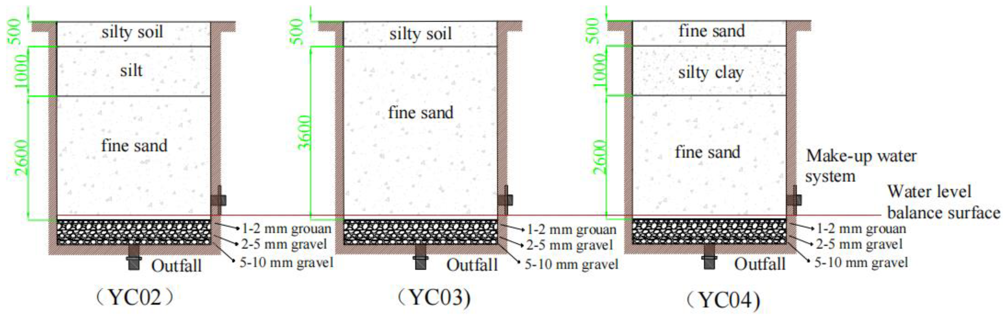
2.2. In Situ Test of Moisture Transport in Heterogeneous Media

At the Ningxia Water and Environment Field Scientific Observation and Research Station, three types of vadose zone models were constructed by artificially backfilling three fiber-reinforced polymer test cylinders (3 × 3 × 4.5 m) based on the typical stratigraphic structure of the study area, including (1) silty soil, silty sand, and fine sand, (2) silty soil and fine sand, and (3) fine sand, silty clay, and fine sand (Figure 2). The dynamic changes in soil water content and water potential vertically and at the interfaces of the layered heterogeneous vadose zone under natural conditions were monitored to study the spatial infiltration characteristics and changing patterns of soil water in the layered heterogeneous vadose zone. The locations and depths of the soil water content and soil water potential monitoring points in the test cylinder at different depths and soil layer interfaces are shown in Figure 3 and

Table 1. Burial depth data of in situ test cylinder monitoring system.

Test Cylinder Number	Monitoring System Burial Depth (cm)
YC02	−10/−20/−30/−40/−60/−80/−100/−120/−140/−160/−260/−380
YC03	−10/−20/−30/−40/−60/−80/−100/−120/−140/−160/−380
YC04	−10/−20/−30/−40/−60/−80/−100/−120/−140/−160/−260/−320/−380

. The soil water content was monitored using ECH2O-5TM (Beijing Duojing Electronic Technology Co., Ltd., Beijing, China) soil moisture sensors with 36 monitoring probes in three test columns. The soil water potential was monitored using eight MPS-6 (Beijing Duojing Electronic Technology Co., Ltd., Beijing, China). The data were automatically tested using a CR1000 Campbell data logger (Beijing Lijia United Technology Co., Ltd., Beijing, China), and the dataset was monitored at 0:00 each day. Mercury negative pressure gauges were regularly drained and replenished to ensure the accuracy of the monitoring data. The data were recorded during the test period from January to September 2022.

3. Model Building

3.1. Basic Equation for Soil Moisture Transport

Using HYDRAS-3D software to establish a three-dimensional profile model, surface evaporation can be ignored due to the small area of the test tube. Without considering the effects of air, temperature, and hysteresis on soil moisture, the soil moisture movement is described as [28] using the modified Van Genuchten equation:

$$\frac{\partial \theta }{\partial t}=\frac{\partial }{\partial x}\left[K\left(h\right)\frac{\partial h}{\partial x}\right]+\frac{\partial }{\partial y}\left[K\left(h\right)\frac{\partial h}{\partial y}\right]+\frac{\partial }{\partial z}\left[K\left(h\right)\frac{\partial h}{\partial z}\right]\pm \frac{\partial K\left(h\right)}{\partial z}$$

(1)

In the equation: θ is the soil volume moisture content (cm³·cm⁻³); T is the infiltration duration (min); K (h) is the unsaturated hydraulic conductivity (cm·min⁻¹); H is the soil water head (cm); and x, y, z are the coordinate axes, where the z-axis is positive (cm).

3.2. Initial and Boundary Conditions

According to the actual observation data of the experiment, the initial conditions of the model are determined. The water head values calculated from the measured water content at depths of 10 cm, 20 cm, 30 cm, 40 cm, 60 cm, 80 cm, 100 cm, 120 cm, 140 cm, 160 cm, and 380 cm in YC02 and YC03 are input into the model as the initial conditions, and the remaining water head is obtained through automatic linear interpolation of the model. The initial conditions are as follows:

$$\begin{gathered} h\left(x,y,z,t\right)=h_0\left(x,y,z\right) \\ x\le X,0\le y\le Y,0\le z\le Z,t=0 \end{gathered}$$

(2)

In the formula, h₀ (x, y, z) is the initial negative pressure head of the soil, cm.

The upper boundary is located on the surface and is designated as the first type of boundary, the atmospheric boundary. The lower boundary condition is set at the water level equilibrium surface, determined as the first type of boundary condition, and set as the fixed water head edge. The initial boundary conditions and head pressure of YC02 and YC03 test cylinders are shown in Figure 4 and Figure 5.

3.3. Model Parameters

In the HYDRAS-3D model, the soil moisture characteristic curve adopts the modified Van Genuchten (VG) [29] model, which is expressed as:

$$\theta \left(h\right)=\left\{\begin{array}{c}{\theta }_r+\frac{{\theta }_s-{\theta }_r}{{\left[1+\left|\alpha h^n\right|\right]}^m} h<0\\ {\theta }_s h\ge 0\end{array}\right.$$

(3)

where ${\theta }_{\left(h\right)}$ is the soil volumetric water content (m³·m⁻³); h is the head pressure (m) (positive in the zone of saturation, negative in the vadose zone, and zero in the phreatic water table); ${\theta }_s$ and ${\theta }_r$ are the saturated water content and residual water content (m³·m⁻³), respectively; α and n are empirical fitting parameters (curve trait parameters), and the unit of measurement of α is cm⁻¹, but n is dimensionless. $m=1-1/n,(0<m<1)$.

The formula for soil unsaturated hydraulic conductivity is as follows:

$$K\left(\theta \right)=K_s\times S^{0.5}{\left[1-{\left(1-S^{\frac{1}{m}}\right)}^m\right]}^2$$

(4)

Among them:

$$S=\frac{\theta -{\theta }_r}{{\theta }_s-{\theta }_r}=\frac{1}{{ (1+{\left|\alpha h\right|}^n)}^m}$$

(5)

In the formula, S represents saturation and K_s is the saturated hydraulic conductivity (cm·min⁻¹). ${\theta }_s$, ${\theta }_r$. K_s was determined through indoor experiments.

According to the negative pressure data obtained from monitoring, the saturated water content and residual water content parameters, α and n in Van Genuchten’s equation, were fitted using MATLAB. The fitted parameters are listed in

Table 2. Fitting parameters of soil moisture characteristic curve.

Test Medium	Fit Parameters
	θr (cm3/cm−3)	θs (cm3/cm−3)	α (cm−1)	n
Silty clay	0.0857	0.4732	0.0079	1.4394
Silty soil	0.0541	0.4545	0.0485	1.6653
silt	0.0552	0.4790	0.0229	1.4717
fine sand	0.0969	0.3595	0.1986	2.4909

.

During the operation of the model, the parameters are adjusted within a certain range using the built-in module of the HYDRAS-3D software. The fitted moisture content is compared with the measured moisture content and continuously modified to make the simulated value as close as possible to the measured value. The hydrogeological parameters of the aeration zone in each test tube were obtained through continuous parameter adjustment, as shown in

Table 3. Soil physical parameters at different depths of each test tube profile.

Number	Buried Depth (cm)	Soil Physical Parameters
		θr (cm3/cm−3)	θs (cm3/cm−3)	α (cm−1)	n	Ks (cm/d)	l (-)
YC02 test tube	0.064 0.057 0.0969	0.064 0.057 0.0969	0.46 0.48 0.3595	0.0985 0.03 0.1986	1.66 1.96 2.68	200 350.2 712.8	0.5 0.5 0.5
YC03 test tube	0.064 0.112	0.064 0.112	0.46 0.3595	0.0485 0.1986	1.66 2.68	200 712.8	0.5 0.5

below.

4. Results and Analysis

4.1. Model Validation

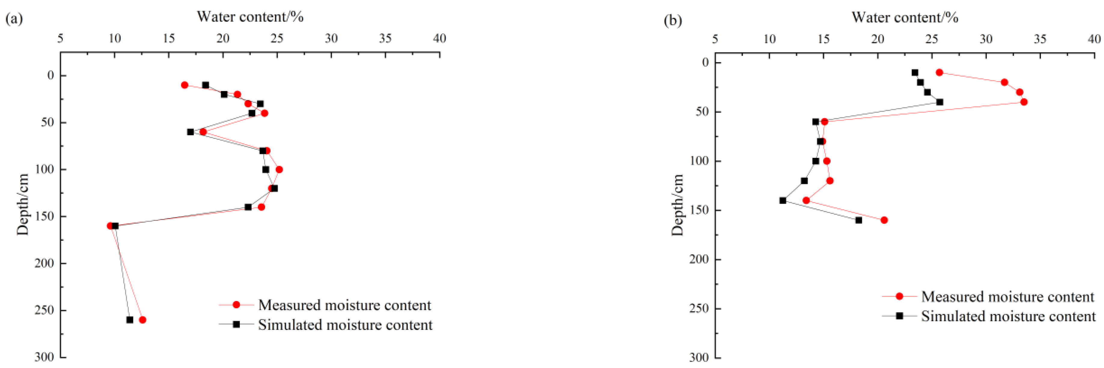
4.1.1. Model Result Validation

Compare the simulated water content values of the model with the measured values of each monitoring point in the aeration zone of the two test tubes, and draw the vertical changes in water content in the identification and validation periods of the two test tubes, as shown in Figure 6 and Figure 7.

From the vertical distribution of water content in the two test cylinders, YC02 and YC03, it can be seen that the trend of simulated and measured water content values tends to be consistent overall, and the fitting effect is good. The decrease in water content at the interface between silt and fine sand is significantly smaller than at the interface between silt and fine sand, indicating that the coarser the particles in the underlying strata, the greater the decrease in water content.

4.1.2. Model Accuracy Verification

Selection decision coefficient R², relative error (RE), and root mean square error (RMES) are used as simulation performance evaluation indicators to comprehensively evaluate the accuracy of the model. R² As a commonly used statistic for the goodness of fit in response simulation, the magnitude of the value represents the relative Chengdu of regression contribution, R² The closer to 1, the better the fit. RE is used to evaluate the degree of fit between measured and simulated values. It is generally believed that when |RE| ≤ 20%, the error between the measured and simulated values is small. RMES is a dimensionless parameter that typically reflects the accuracy of the model. A smaller RMES represents a better fitting effect.

The determination coefficients, relative errors, and root mean square errors between the simulated values of the model during the identification and validation periods and the measured values in the experiment are shown in

Table 4. Statistical table of the fitting effect of soil moisture content at different burial depths of the test tube.

Number	Buried Depth (cm)	R2	|RE| (%)	RMSE
YC02 test tube	0~50 50~150 100~400	0.769 0.958 0.986	0.990 3.650 2.660	0.0221 0.0178 0.0097
YC03 test tube	0~50 50~400	0.629 0.859	10.46 2.170	0.0249 0.0200

.

There is a difference between the measured values of water content in each soil layer of the YC02 and YC03 test tubes and the simulated values of the model, R² > 0.5, |RE| < 20%, RMES < 0.025. The simulation value of the model fits well with the measured value of the test tube, and the accuracy of the model meets the requirements. In complex heterogeneous media aeration zones, it can reflect the trend of soil moisture content changes at different depths to a certain extent. Among them, the YC02 test tube has the best performance in various indicators of the fine sand layer buried at a depth of 100–400 cm, indicating that the error between the measured and simulated soil moisture content values within this buried depth range is the smallest.

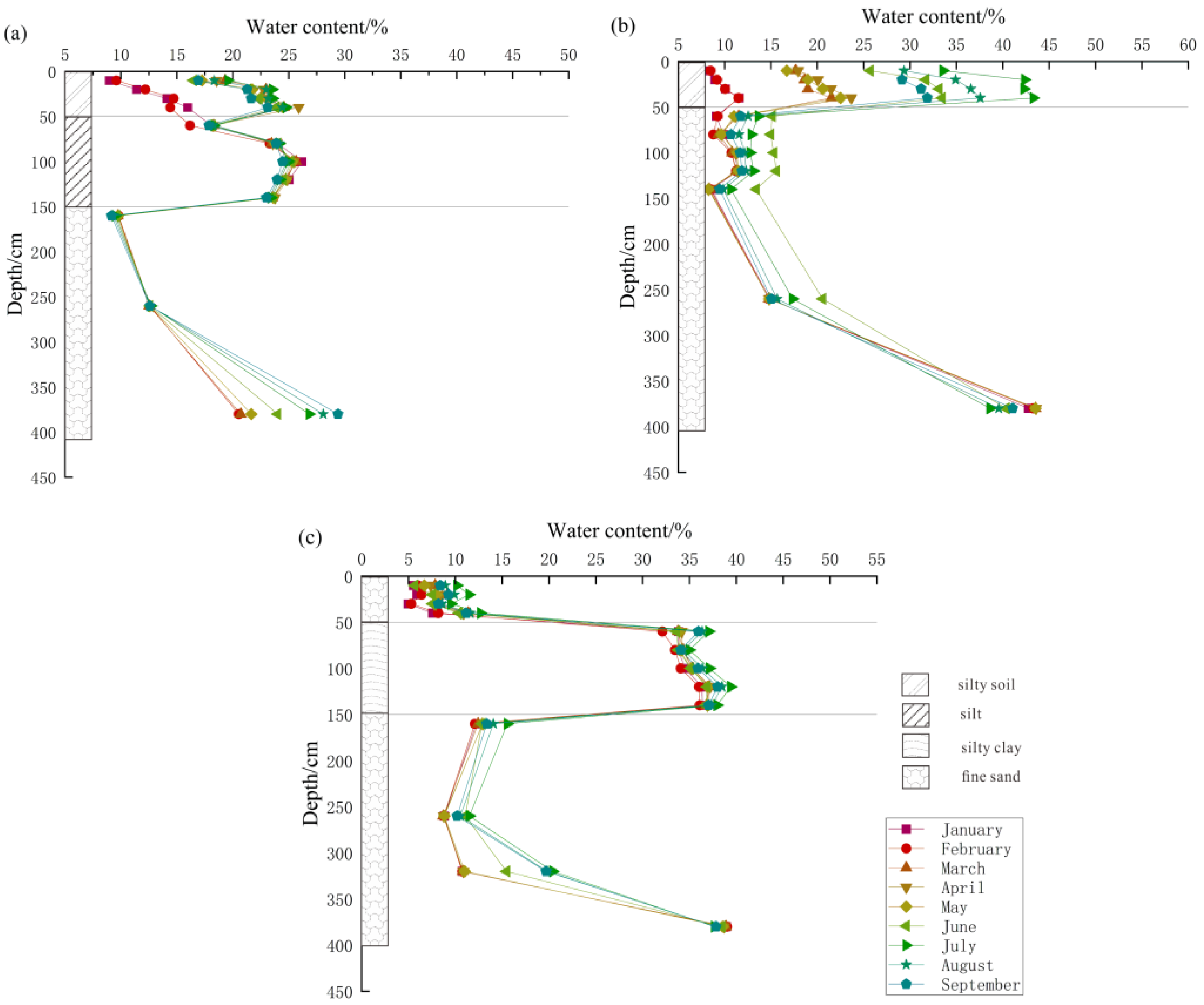
4.2. Influence of a Layered Heterogeneous Structure on Water Movement in the Vadose Zone

The vertical variation in soil moisture in the vadose zones of the three test cylinders from January to September 2022 is shown in Figure 8.

Figure 8a shows that the water content in the silty soil layer above 50 cm in the YC02 test cylinder increased with time with a notable magnitude of change. The size and magnitude of the changes in water content in January and February were small, probably due to freezing and thawing. The maximum water content of the silty soil layer was 25.9% during April. The water content of the silty sand layer (50–150 cm) was >20%. The maximum water content of YC02 was 26.2% at a burial depth of 120 cm in January. The water content of the fine sand layer below 150 cm exhibited a small change of <20%. The water content of the silty clay–silty sand and silty soil–silty sand interfaces at a depth of 50 cm, and that of the silty sand–fine sand interface at a depth of 150 cm decreased significantly.

As shown in Figure 8b, the water content of the clay soil layer above 50 cm in the YC03 test cylinder was low from January to February due to the influence of freeze-thaw action, and it started to increase substantially in March, reaching a maximum of 43.3% in July. The water content of the silty soil–fine sand interface at a burial depth of 50 cm decreased significantly. The water content of the fine sand layer below 50 cm was lower (<20%), although the change was not significant. The water content of the fine sand layer above 50 cm in the YC04 test cylinder, shown in Figure 8c, was low at approximately 10%, and the rate of change was not notable. The water content at 50 cm from the fine sand–silty clay interface increased substantially. The water content in the 50–150 cm silty clay layer remained at approximately 35%, with no notable change. At 150 cm, the water content of the silty clay–fine sand interface decreased to 15%, and the change in the fine sand layer was not notable below 150 cm. The abrupt increase in water content near a depth of 400 cm in the three test cylinders was due to the proximity to the water level equilibrium surface.

In general, water content at the soil–layer interface changed abruptly, and that at the interface of the “upper fine and lower coarse” materials, such as silty soil–silty sand, silty soil–fine sand, and silty clay–fine sand, decreased considerably because the overlying layer had a strong water-holding capacity. To facilitate the downward movement, water must accumulate at the interface of the soil layers until it surpasses the water-holding capacity of the overlying layer. The water content in the coarse and fine upper coarse structures of the fine sand–silty clay interface increased substantially because the water-holding capacity of the overlying layer was weak, and the water absorption capacity of the underlying layer was strong, causing the water in the overlying layer to move faster to the underlying layer.

4.3. Profile Water Content Variability Characteristics

The coefficient of variation (CV) values of the water content of the three test cylinder profiles at different depths at different times were analyzed using IBM SPSS (SPSS-Statistics-25) software, and the CV values of the soil water content of the test cylinder profiles were plotted against time and in contour plots, as shown in Figure 9 and Figure 10.

Figure 9 and Figure 10 show that in the three test cylinders, above the 60–80 cm burial depth, the soil moisture content changed more from January to March because of the influence of the freezing capacity, resulting in a larger CV value (between 5 and 20%), with a larger fluctuation and more frequent vertical exchange of water. The YC03 test cylinder from April to May and from July to September and the YC02 and YC04 test cylinders from April to September were not significantly affected by rainfall, with CV values of soil moisture content at 5% or lower. The YC03 test cylinder was significantly affected by rainfall in June, resulting in a large variation in the soil moisture content in that month. The CV value in the entire profile increased, mainly by >30%, with the maximum reaching 59.11%. Based on the CV variation, the vertical transport of soil moisture in the profiles can be classified as follows: (I) stable period (April to September, when soil moisture was not significantly affected by rainfall or freezing and thawing); (II) slow change period (January to March, when soil moisture was affected by freezing); and (III) rapid rainfall change period (June, when YC03 was significantly affected by rainfall).

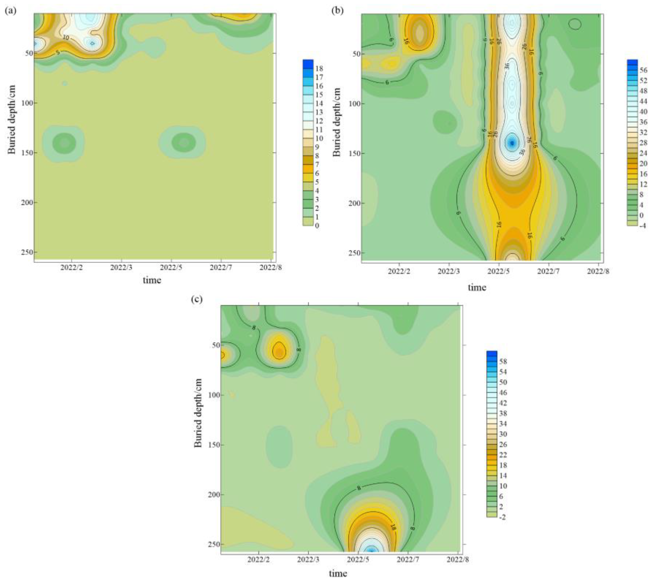
4.4. Spatial and Temporal Distribution Characteristics of the Water Movement in the Layered Heterogeneous Vadose Zone

Using the modified Van Genuchten (VG) model formula, calculate the negative pressure of each monitoring point at the interface of the test tube and use the bottom of the test tube as the coordinate origin to obtain the soil water potential at each interface. Calculate the gradient of the soil water potential at the interface over time.

The locations of the monitoring points within each plane are shown in Figure 11. The contour plots and change gradients of soil water potential from January to September in 10 planes were plotted for the YC02 test cylinder at burial depths of 40, 60, 140, and 160 cm, for the YC03 test cylinder at burial depths of 40 and 60 cm, and for the YC04 test cylinder at burial depths of 40, 60, 140, and 160 cm (Figure 12, Figure 13, Figure 14, Figure 15, Figure 16 and Figure 17).

The YC02 test cylinder soil water potential in January and February ranged from 50 to −280 cm at a buried depth of 40 cm, above and below the silty soil–silty sand interface and in the plane of the silty soil layer (Figure 12a). The soil water movement direction in the plane was 1#, 2#→4#, 5#→8#, 9#, and the soil water potential from March to September ranged from 280 to −320 cm, and the soil water movement direction was as follows: 4#, 5# →1#, 2#, 7#, 8#, 9#→1#, 2#, 3#. Thus, the water movement direction in the first two months was directly opposite to that in March–September. Figure 13a shows that the temporal change gradient of the soil water potential in the plane in February and March was 5.14 cm/day, which was greater than that in the other stages. Plane evaporation and infiltration were not uniform, and a zero-flux surface was observed during this period, with a notable change in lateral water movement, indicating that the lateral movement of soil moisture during this period was influenced by the soil–layer interface. Figure 12b shows that the soil moisture moved from 5# to the surrounding monitoring points from January to September in the plane of the silt layer at a burial depth of 60 cm. Figure 13b shows that the temporal change gradients of soil water potential between January and February, as well as between February and March, were larger than those at other stages (−12.79 and 14.29 cm/day, respectively). The evaporation and infiltration in this plane were not uniform, but there was no significant change in the lateral water movement, indicating that the lateral soil water movement in this plane was barely affected by the soil–layer interface.

Figure 12c shows that above and below the silty sand–fine sand interface of the YC02 test cylinder in the silty sand layer plane at a burial depth of 140 cm, the soil water movement directions were 2#, 4#→other monitoring points from January to May and August to September, and 5#→ (surrounding monitoring points in June). The direction of water movement in June differed significantly from that of the other eight months. Figure 13c shows that the time gradient of the soil water potential in the plane was small, ranging from −0.93 to 0.01 cm/day, and moisture evaporation and infiltration were more uniform. However, a zero-flux surface was observed in May–June and June–July when there was a notable trend of lateral moisture transport, indicating that lateral soil moisture transport during these two time periods was influenced by the soil–layer interface. Figure 12d shows that the soil water movement direction in the fine sand layer plane at a burial depth of 160 cm was more complex: 1# and 9#→other monitoring points in January; 1#–3#→7#–9# in February and March; 7#–9#→1#–3# in April, which was opposite to the direction in February and March; surrounding monitoring points→5# in May; 7#→other monitoring points in June; 3#→other monitoring points in July, which was almost opposite to June; and 3#, 5#, 7#→other monitoring points in August and September. From Figure 13d, the time gradient of soil water potential in the plane was between −5.41 and 3.9 cm/day, evaporation and infiltration were relatively uneven, and the lateral transport of water in the plane was variable, indicating that the lateral transport of soil water was greatly influenced by the soil–layer interface.

Figure 14a shows that above and below the silty soil–fine sand interface in the YC03 test cylinder, in the silty soil layer plane at a burial depth of 40 cm, the soil water movement direction was the other monitoring points → 4# from January to May and 3# → 7# from June to September. Figure 15a shows that the temporal change gradient of the soil water potential between February and March was larger than that of the other stages. At 8.54 cm/day, the evaporation and infiltration in the plane were not uniform, and the lateral movement of soil water between May and June changed slightly, indicating that the lateral soil water movement during this period was affected by the soil–layer interface to a small extent. Figure 14b shows that the soil water movement direction in the plane of the fine sand layer at a burial depth of 60 cm was 2#→4# in January, surrounding monitoring points→5# in February, and 3#→5#→7# from March to September. Figure 15b shows that the gradient of temporal change in soil water potential in the plane was between −0.77 and 1.09 cm/day, and evaporation and infiltration were more uniform. However, a significant change in lateral soil water movement from January to March was observed, which indicated that the lateral soil water movement during this period was influenced by the soil–layer interface to a certain extent.

Figure 16a shows that above and below the fine sand–silty clay partition interface in the YC04 test cylinder, in the fine sand layer plane at a burial depth of 40 cm, the soil water movement direction was 1#→5#→9# in January and February; 9#→3# and 9#→6# in March and April; 1#→3# and 9#→3# in May and 9 June #→6# in July, and 5#→3# in August and September. Figure 17a shows that the gradient of temporal change in soil water potential in the plane was between −0.4 and 0.82 cm/day, and evaporation and infiltration were more uniform. However, the lateral transport of soil water was more complicated, indicating that the lateral transport of soil water in this plane was greatly influenced by the soil–layer interface. Figure 16b shows that in the silty clay layer at a burial depth of 60 cm, there was no significant change in the direction of lateral transport of soil water from January to March and from April to September, which was 3#→1# and 1–3#→7–9#. The only direction in April was 5#→ the surrounding monitoring points. Figure 17b shows that the gradient of the temporal change in soil water potential in the plane was between −19.9 and 17.8 cm/day, evaporation and infiltration were not uniform, there was a zero-flux surface in March–April and April–May, and there was a notable change trend of moisture lateral transport, indicating that the lateral transport of soil moisture during this period was greatly influenced by the soil–layer interface.

Figure 16c shows that above and below the silty clay–fine sand partition interface in the YC04 test cylinder, in the plane of the silty clay layer at a burial depth of 140 cm, the soil water movement direction was 3#→1#, 3#→7#, and 3#→9# in January, and surrounding monitoring points→2# from February–September. Figure 17c shows that the gradient of temporal change in soil water potential between January and February was greater than that of the other stages at −2.57 cm/day, and a zero-flux surface was observed during this period. There was a notable change in the lateral water movement, indicating that the lateral soil moisture transport during this period was greatly influenced by the soil–layer interface. Figure 16d shows that the soil water potential in the fine sand layer plane at a burial depth of 160 cm was mostly between 209 and 265 cm, and the direction of soil water movement was 3#→1#, 3#→7#, and 3#→9# in January, and 7#→1#, 7#→3#, and 7#→9# in February–September (opposite to January). Figure 17d shows that the gradient of the soil water potential change was between −0.26 and 0.25 cm/day, and evaporation and infiltration were more uniform, but there was a zero-flux surface between January and February. During this period, the change in the lateral water movement exhibited a distinct trend, indicating the substantial influence exerted by the soil–layer interface during this period.

In general, according to the soil water potential gradient change and contour diagrams, the soil water evaporation and infiltration in the plane at the soil–layer interface was relatively uneven. The maximum value of the soil water potential change gradient of −19.9 cm/day appeared in the silty clay plane at a 60 cm burial depth in the YC04 test cylinder from January to February. This was followed by a 17.8 cm/day gradient in the silty clay plane at a 60 cm burial depth in the YC04 test cylinder from February to March. Therefore, the two highest values occurred in the silty clay planes. The lateral movement of soil water is affected by the soil–layer interface. The different soil layers above and below the soil–layer interface were affected differently, as was the time at which they were affected. The fine-sand layer was most notably affected by the soil–layer interface, followed by the silty and silty clay layers. The silty-sand layer was the least affected by the soil–layer interface.

5. Discussion

On the basis of in situ testing of water transfer in heterogeneous media, this article monitors the distribution of water content in the vadose zone of layered heterogeneous media. A three-dimensional model of water transport in the vadose zone of layered heterogeneous media was constructed using the HYDRAS-3D (V 2.x) software, and the accuracy of the model was verified. The vertical distribution and variability characteristics of soil water in the vadose zone of layered heterogeneous structure were analyzed, revealing the spatiotemporal distribution characteristics of lateral water transport at the soil layer boundary. The results indicate that the established HYDRAS-3D model has high accuracy and certain reliability. At the soil–layer interface, the vertical distribution of moisture in the aeration zone will undergo a sudden change, and the variability of water content will significantly change. The horizontal migration and evaporation infiltration of water in the plane are significantly affected by the heterogeneous structure, but the degree of influence varies greatly among different lithologies. In addition to the HYDRAS software, machine learning technology also has good applicability in simulating soil moisture transport. Among them, the Extreme Gradient Boost (XGBoost) algorithm is the preferred method, with good efficiency and scalability [30]. In future research, the two simulation methods can be compared and analyzed to further improve the accuracy of soil moisture transport models.

6. Conclusions

An in situ test of water movement in heterogeneous media consisting of silty soil, silty sand, fine sand, and silty clay with different soil–layer sequences and thicknesses was developed, and a monitoring system was installed at different depths and soil–layer interfaces to continuously monitor soil moisture content and negative pressure. Using the obtained data, a three-dimensional model of water transport in the vadose zone of layered heterogeneous media was constructed using the HYDRAS-3D software, and the accuracy of the model was verified. The vertical distribution and variability characteristics of soil water in the vadose zone of the layered heterogeneous structure were analyzed, revealing the spatiotemporal distribution characteristics of lateral water transport at the soil layer boundary. The results indicate that:

(1)

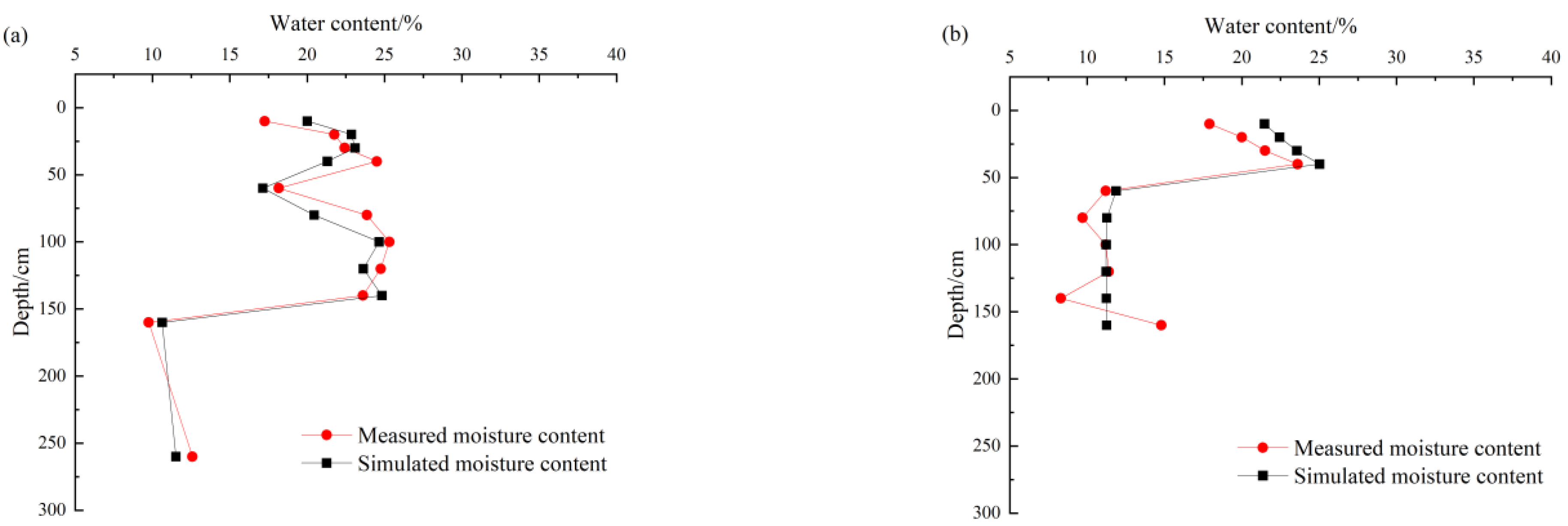
Comparing and analyzing the simulated and measured values in the HYDRAS-3D model, the two showed good consistency, verifying the accuracy and reliability of the model, indicating that the model can be applied well in experiments.

(2)

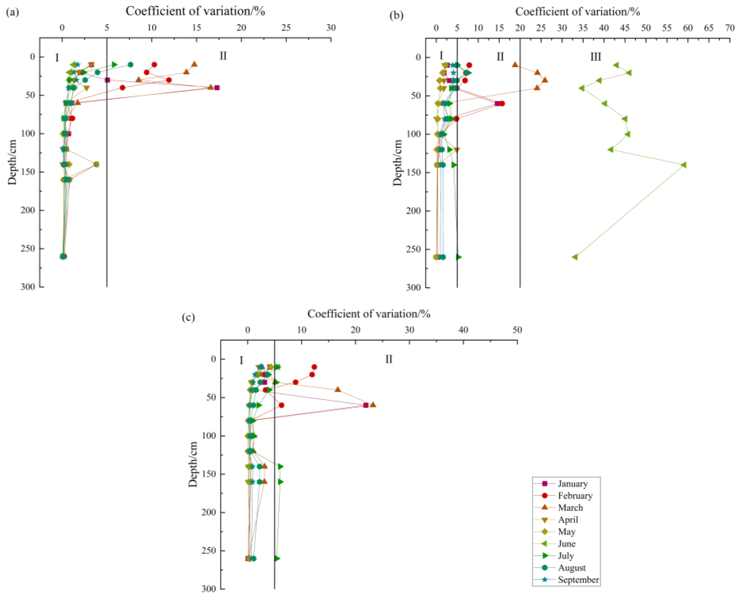
The water content at the interface of the soil layer will undergo a sudden change. Expressing the characteristics of water content variability more accurately in the test cylinder profiles, water movement in the vadose zone was divided into the following stages: (I) stable period, (II) slow change period, and (III) rainfall rapid change period. From April to May and July to September in the YC03 test cylinder, which was not significantly affected by rainfall, and from April to September in the YC02 and YC04 test cylinders, the CV of the soil moisture content was 5% or less, and water movement in the vadose zone was in the (I) stable period. The CV of the soil moisture content of the three test cylinders from January to March was mostly between 5 and 20%, with large fluctuations and frequent moisture exchanges in the vertical direction, particularly from 60 to 80 cm. In June, the YC03 test cylinder, which was significantly affected by rainfall, had a CV of water content in the entire profile of >30% and a maximum value of 59.11% when the water movement in the vadose zone was in the (III) rainfall rapid change period.

(3)

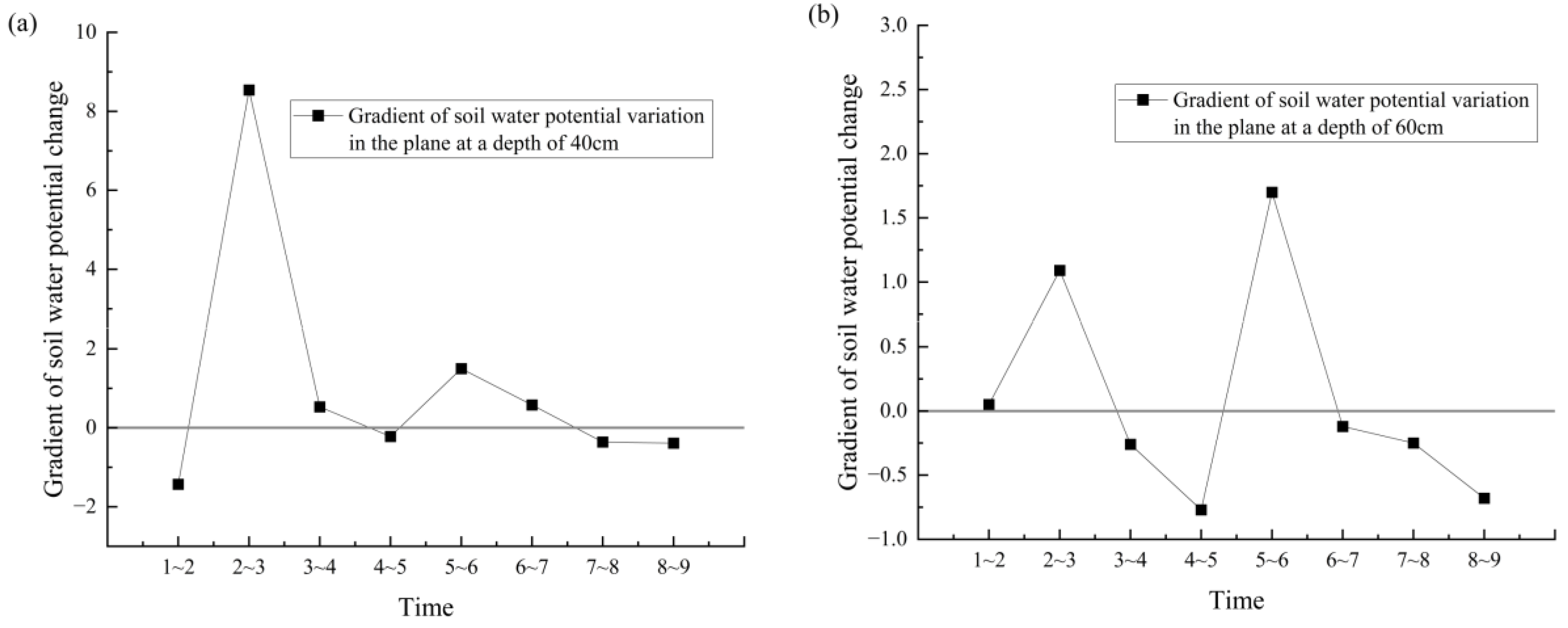
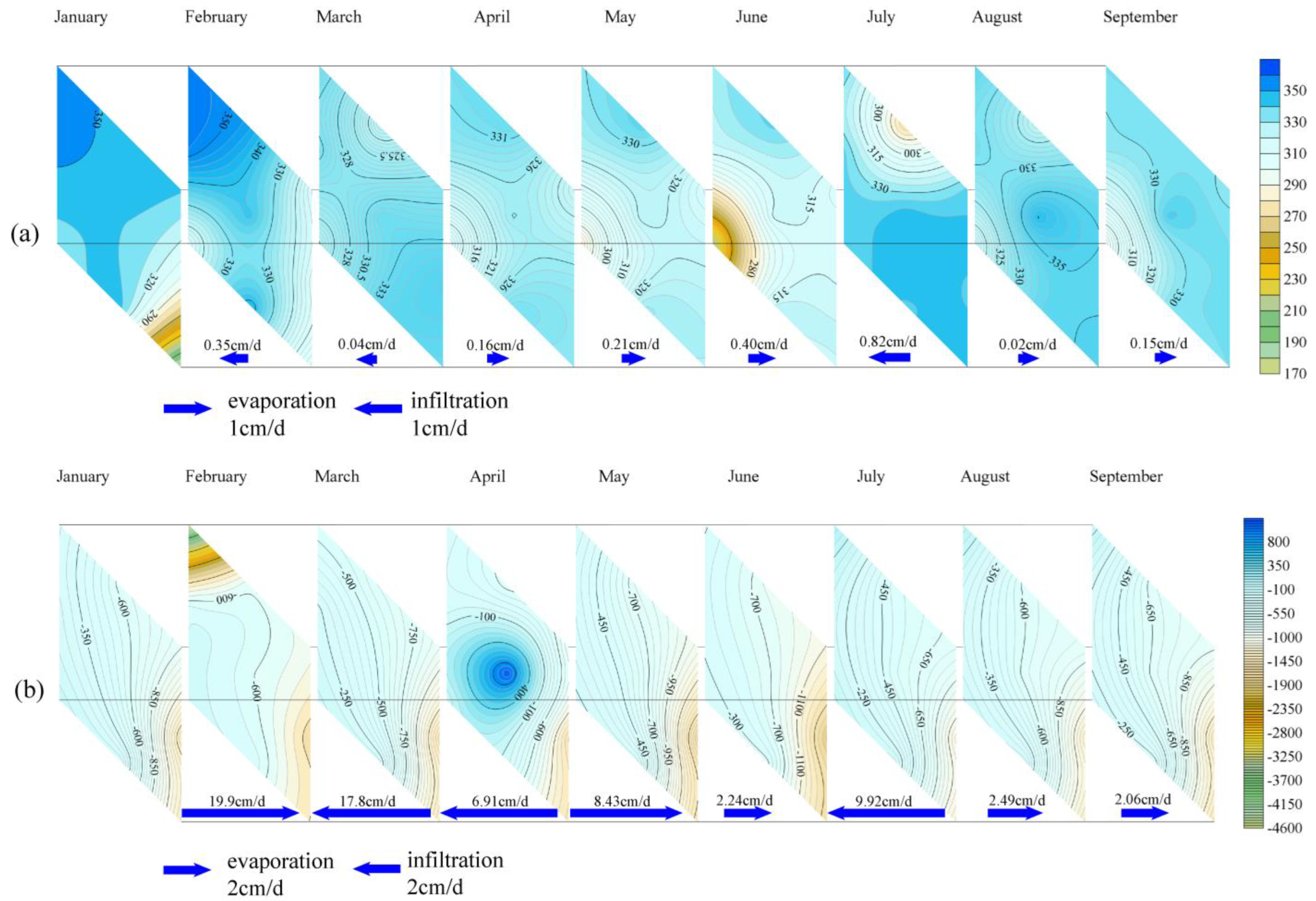
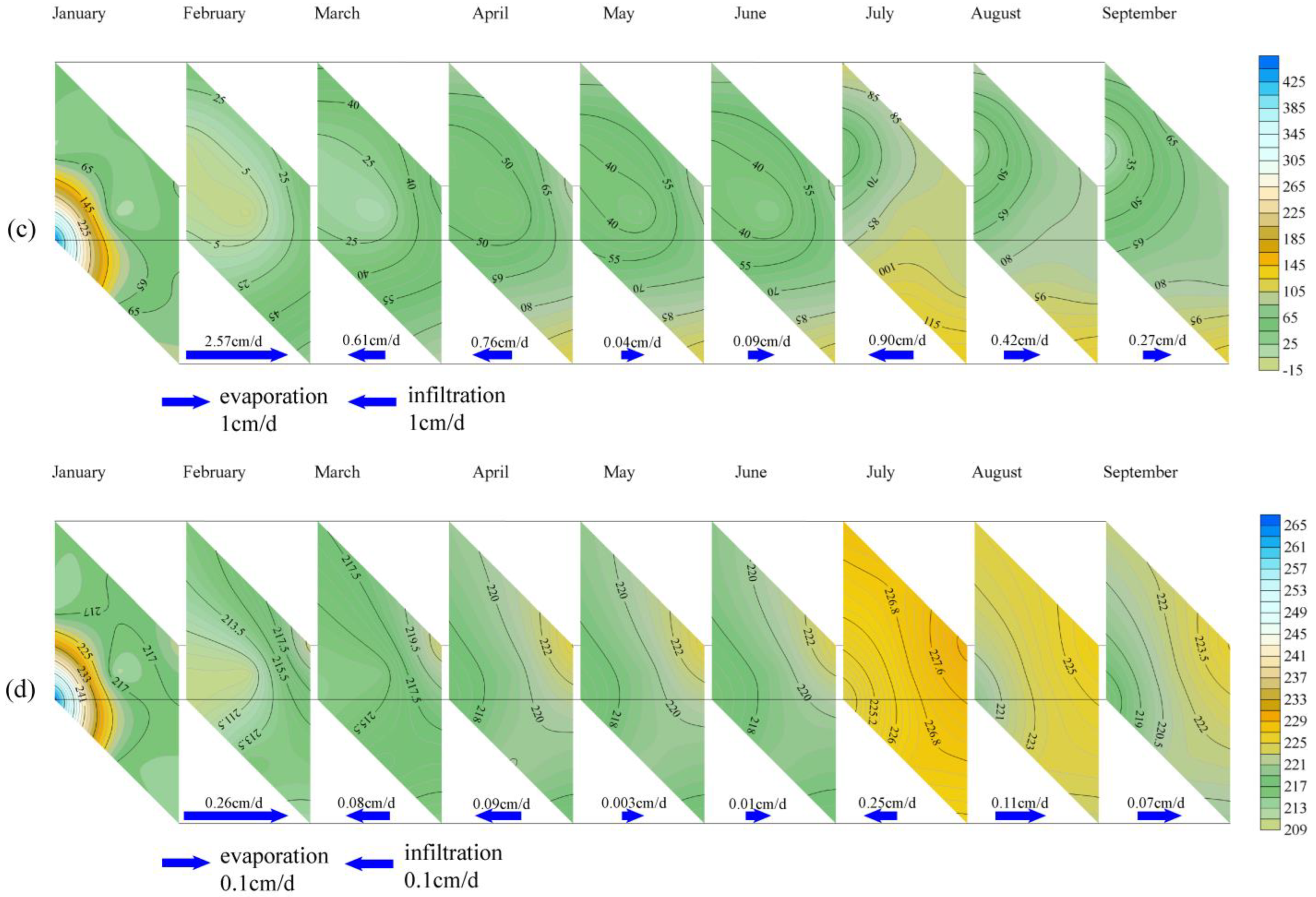
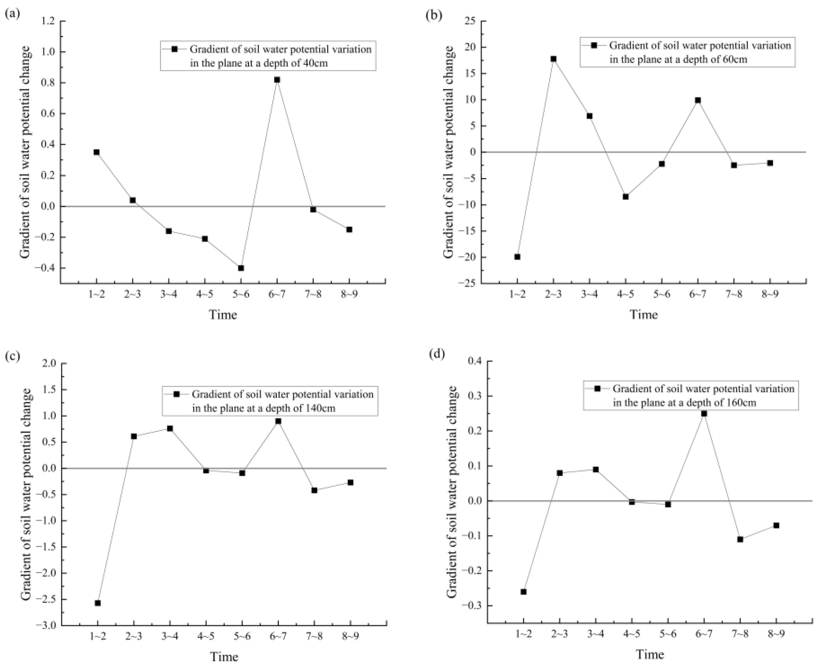
The two largest values (19.9 and 17.8 cm/day) of the temporal change gradient of the soil water potential were observed in the silty clay layers of the YC04 test cylinder. The influence of the soil–layer interface on evaporation and infiltration in the silty clay layer was the most pronounced.

(4)

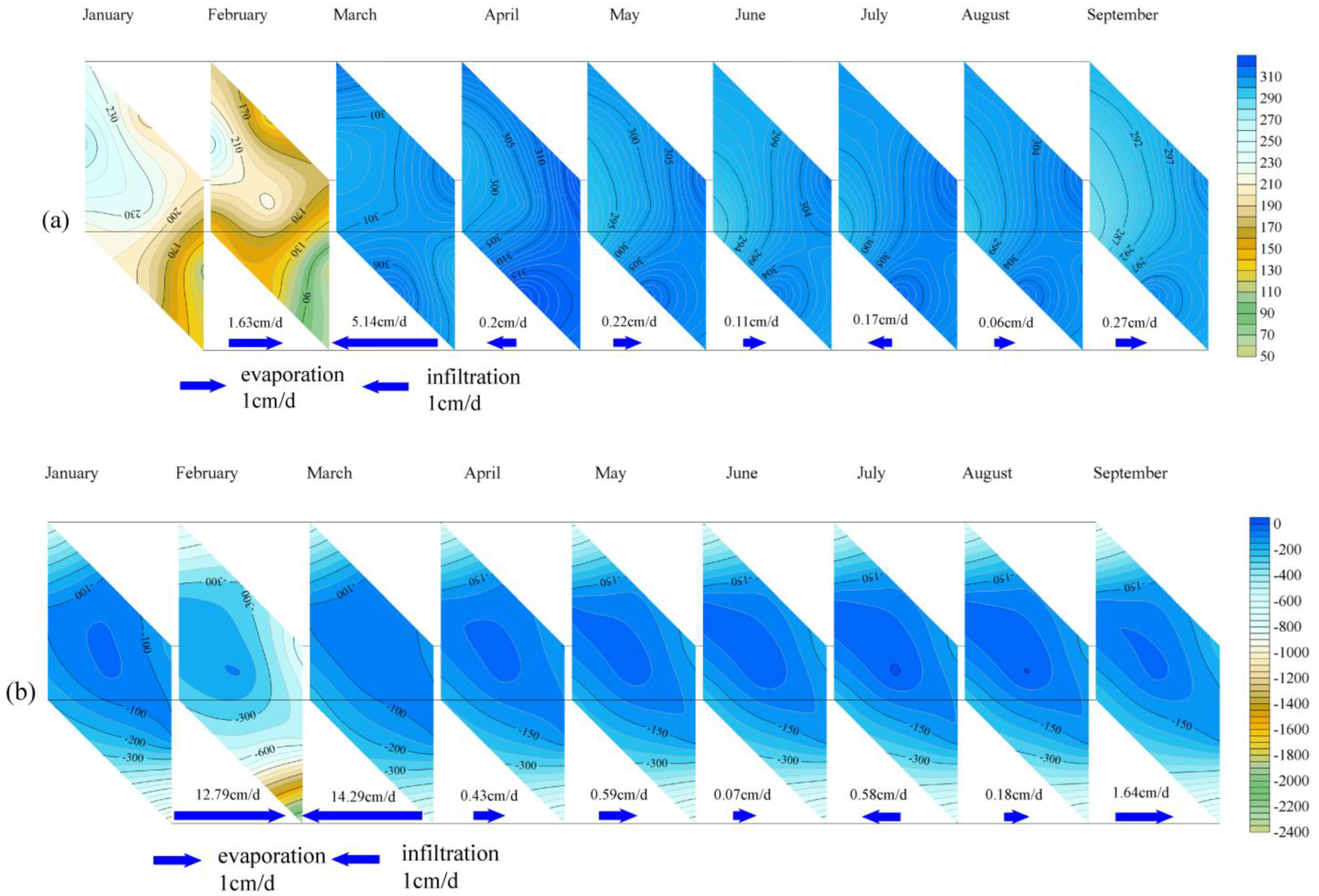
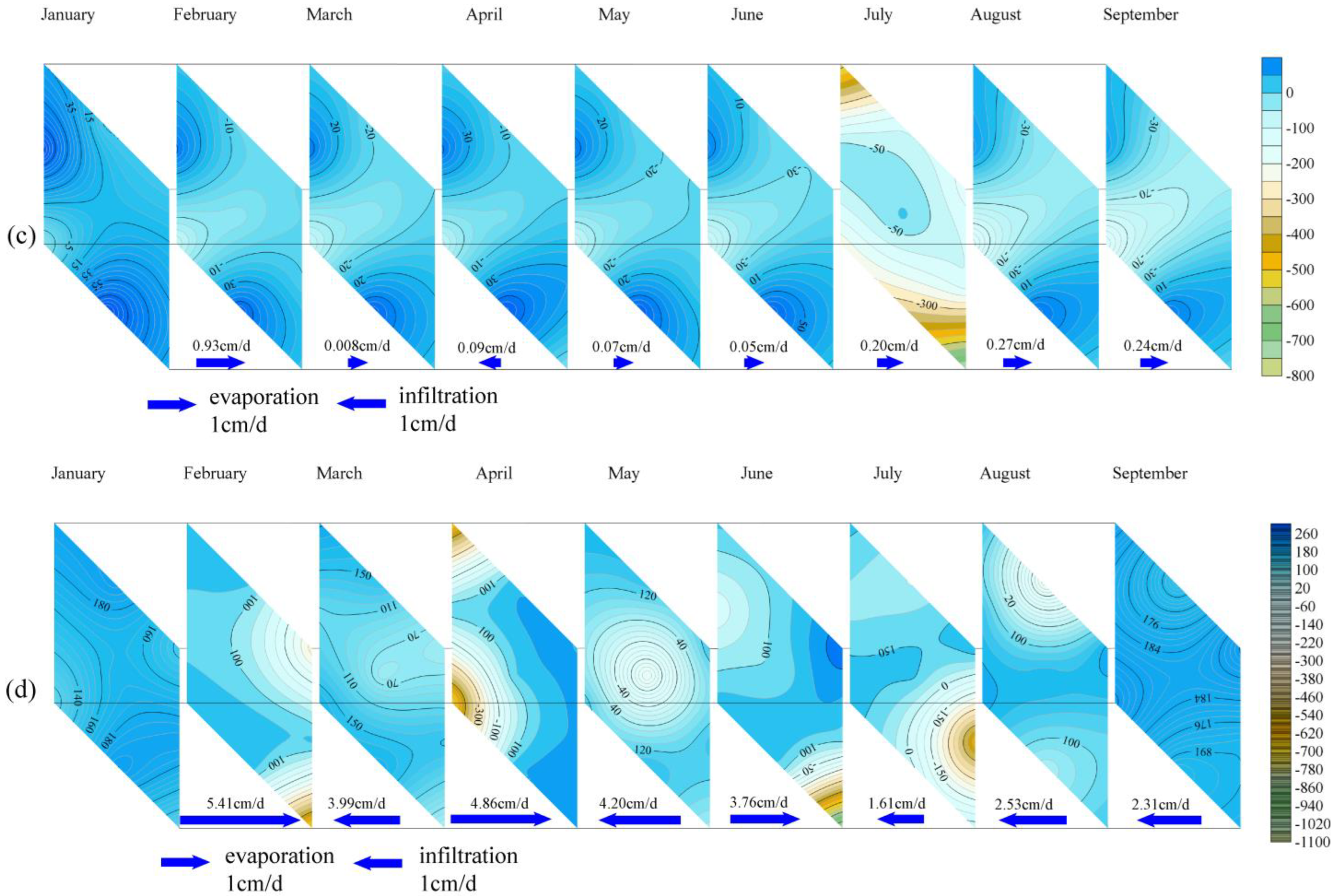
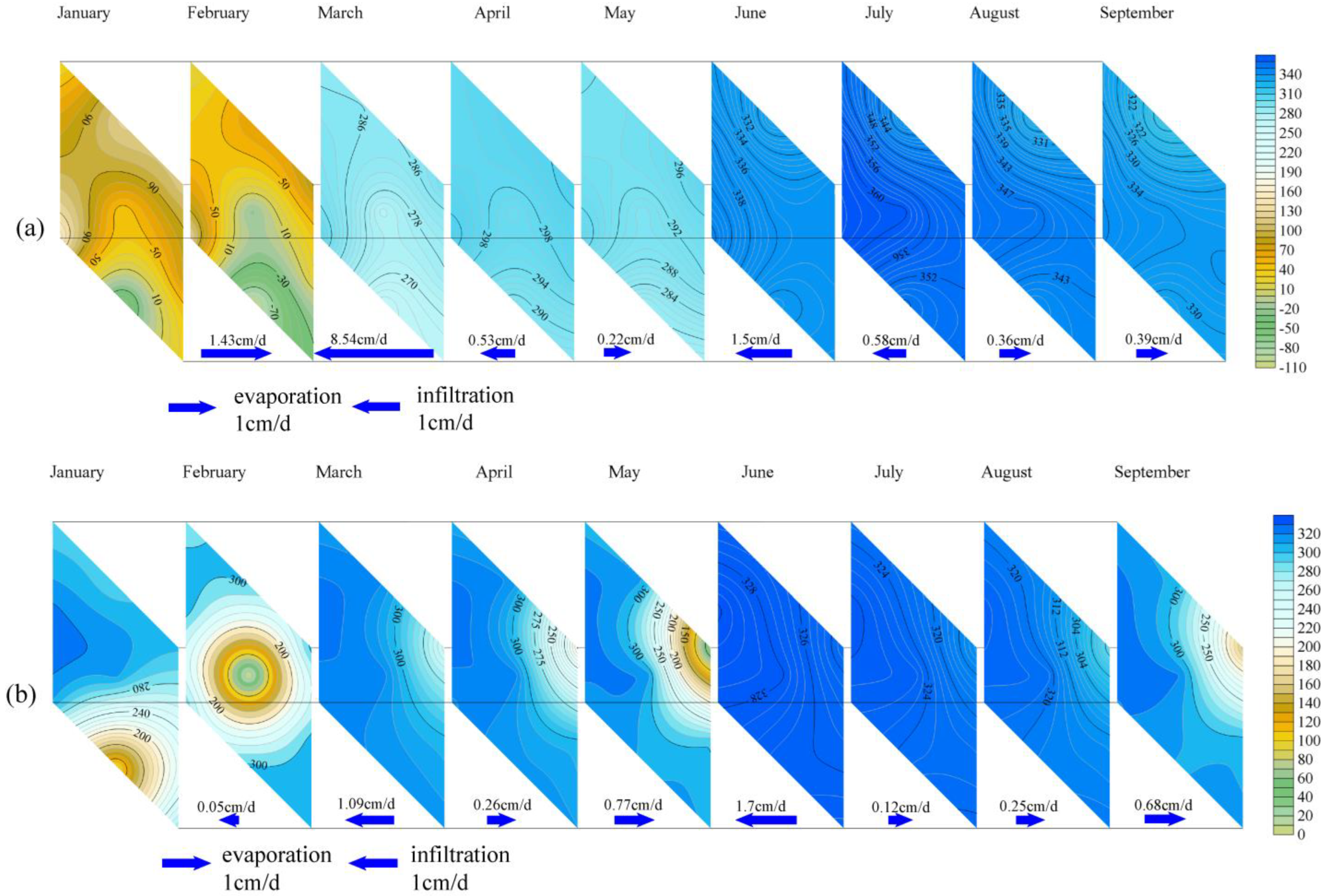
The lateral movement of soil moisture in the plane at the interface was also affected to some extent by the layered heterogeneous structure, with the degree and time affected by the differences in the soil layers above and below the interface. The fine sand layer was the most affected by the soil–layer interface, followed by the silty soil and silty clay layers. The silty sand layer was the least affected by the soil–layer interface.

This article only uses soil temperature and humidity sensors as a monitoring method in the moisture monitoring of the vadose zone and is limited to analyzing the water transport situation in heterogeneous media and constructing a three-dimensional model. The vadose zone is a three-phase structure of gas liquid solid, and multiple methods can be used to verify the monitoring data in future research and further improve the research on gas movement in the vadose zone of heterogeneous media.

References

1. Edmunds, W.M.; Tyler, S. Unsaturated zones as archives of past climates: Toward a new proxy for continental regions. Hydrogeol. J. 2002, 10, 216–228. [Google Scholar] [CrossRef]
2. Gong, Z.N.; Gong, H.L.; Deng, W. An overview of water movement in groundwater -Soil-Plant-Atmosphere continuum with shallow water table. J. Agro-Environ. Sci. 2006, 25, 365–373. [Google Scholar]
3. Ji, X.B.; Kang, E.S.; Zhao, W.Z. Simulation of heat and water transfer in a surface irrigated, cropped sandy soil. Agric. Water Manag. 2009, 96, 1010–1020. [Google Scholar] [CrossRef]
4. Li, Q.; Wang, Z.; Shangguan, W.; Li, L.; Yao, Y.; Yu, F. Improved daily SMAP satellite soil moisture prediction over China using deep learning model with transfer learning. J. Hydrol. 2021, 600, 126698. [Google Scholar] [CrossRef]
5. Liu, W.; Wang, J.; Xu, F.; Li, C.; Xian, T. Validation of Four Satellite-Derived Soil Moisture Products Using Ground-Based In Situ Observations over Northern China. Remote Sens. 2022, 14, 1419. [Google Scholar] [CrossRef]
6. Dabrowska-Zielinska, K.; Budzynska, M.; Tomaszewska, M.; Malinska, A.; Gatkowska, M.; Bartold, M.; Malek, I. Assessment of Carbon Flux and Soil Moisture in Wetlands Applying Sentinel-1 Data. Remote Sens. 2016, 8, 756. [Google Scholar] [CrossRef]
7. Hutchinson, J.S.; Vought, T.J.; Hutchinson, S.L. Continuous soil moisture mapping using MODIS NDVI and LST products. Pap. Appl. Geogr. Conf. 2006, 29, 140–149. [Google Scholar]
8. Dabrowska-Zielinska, K.; Budzynska, M.; Tomaszewska, M.; Bartold, M.; Gatkowska, M.; Malek, I.; Turlej, K.; Napiorkowska, M. Monitoring Wetlands Ecosystems Using ALOS PALSAR (L-Band, HV) Supplemented by Optical Data: A Case Study of Biebrza Wetlands in Northeast Poland. Remote Sens. 2014, 6, 1605–1633. [Google Scholar] [CrossRef]
9. Zhao, G.Z. Study on Transgormation Mechanism of Vadose Zone Water-Groundwater in the Wind-Blown Sand Area of the Ordos Basin; Chang’an University: Xi’an, China, 2011. [Google Scholar]
10. Xu, Y.Z.; Zhao, G.Z.; Mu, N.S. Review on factors affecting the process of water movement in vadose zone. J. N. China Univ. Water Resour. Electr. Power Nat. Sci. Ed. 2019, 40, 37–41. [Google Scholar]
11. Li, Y.; Ren, X.; Robert, H. Influence of various soil textures and layer positions on infiltration characteristics of layered soils. J. Drain. Irrig. Mach. Eng. 2012, 30, 485–490. [Google Scholar]
12. Miller, D.E.; Gardner, W.H. Water infiltration into stratified soil. Soil Sci. Soc. Am. J. 1962, 26, 115–119. [Google Scholar] [CrossRef]
13. Hill, D.E.; Parlange, J.Y. Wetting front instability in layered soils. Soil Sci. Soc. Am. J. 1972, 36, 697–702. [Google Scholar] [CrossRef]
14. Chen, J.; Huang, G.H.; Huang, Q.Z. Simulation of one-dimensional solute transport in homogeneous and heterogeneous soils with scale-dependent fractional advection-dispersion equation. Adv. Water Sci. 2006, 3, 299–304. [Google Scholar]
15. Yu, S.P.; Yang, J.S. Effect of clay interlayers on soil water-sait movement in easily-salinized regions. Adv. Watter Sci. 2011, 22, 495–501. [Google Scholar]
16. Wang, W.Y.; Wang, Q.J.; Shen, B.; Zhang, J.F. Infiltration characteristics of soil with double layer structure in Qinwangchuan area of Gansu Province. J. Soil Eros. Water Conserv. 1998, 2, 37–41. [Google Scholar]
17. Li, J.S.; Yang, F.Y.; Li, Y.F. Water and nitrogen distribution under subsurface drip fertigation as affected by layered-textural soils. Trans. CSAE 2009, 25, 25–31. [Google Scholar]
18. Wang, Q.J.; Wang, Z.R.; Zhang, J.F. Infiltration mechanism of layered soil and its simulation model. Shui Li Xue Bao 1998, S1, 77–80. [Google Scholar]
19. Zettl, J.D.; Barbour, S.L.; Huang, M. Influence of textural laying on field capacity of coarse soils. Can. J. Soil Sci. 2011, 91, 133–147. [Google Scholar] [CrossRef]
20. Li, Y.T.; Wang, W.K.; Xiao, J.Y.; Yang, X.T. Field test of moisture migration in vadose zone under heterogeneity. J. Saf. Environ. 2012, 12, 134–137. [Google Scholar]
21. Cui, H.H.; Zhang, G.H.; Zhang, Y.Z.; Zhang, B.; Feng, X.; Lang, X.J. Soil water-holding properties of different soil body configuration. Agric. Res. Arid Areas 2020, 38, 1–5. [Google Scholar]
22. Xu, Z.Q.; Mao, X.M.; Chen, S. Tank experiment on the influence of the sequence alignment on water movement in multi-layered soil. China Rural. Water Hydropower 2016, 8, 59–62. [Google Scholar]
23. Shang, J. Water Dynamics of Vadose Zone in Badan Jaran Desert; China University of Geosciences: Beijing, China, 2014. [Google Scholar]
24. Meng, L.Q.; Nie, Z.L. Simulation of Water Migration in Unsaturated Zone in Typical Area of Wuwei Basin. J. Agric. Catastrophol. 2021, 11, 146–149+151. [Google Scholar]
25. Liu, Z.X. Study on the Law of Water Migration in the Aeration Zone of Minqin Basin; China University of Geosciences: Beijing, China, 2020. [Google Scholar]
26. Dai, Z.G. Numerical simulation of soil water movement in free infiltration under surge-root irrigation in red soil region based on Hydrus-2D. Agric. Res. Arid Areas 2020, 38, 27–31. [Google Scholar]
27. Xu, J.Z.; Liu, W.X. Simulation of Soil Moisture Movement under Negative Pressure Micro-irrigation Based on HYDRUS-2D. Trans. Chin. Soc. Agric. Mach. 2021, 52, 287–296. [Google Scholar]
28. Li, C.Y.; Ren, L.; Li, B.G. Parametric Estimation of the Van Genuchten’s Equation by the Optimization Method. Adv. Water Sci. 2001, 12, 473–478. [Google Scholar]
29. Van Genuchten, M.T. A closed-form equation for predicting the hydraulic conductivity of unsaturated soils. Soil Sci. Soc. Am. J. 1980, 44, 892–898. [Google Scholar] [CrossRef]
30. Bartold, M.; Kluczek, M. A Machine Learning Approach for Mapping Chlorophyll Fluorescence at Inland Wetlands. Remote Sens. 2023, 15, 2392. [Google Scholar] [CrossRef]
Figure 1. Schematic diagram of the study area location.
Water 15 03550 g001
Figure 2. Schematic diagram of filling structure of heterogeneous medium moisture transfer test tube.
Water 15 03550 g002
Figure 3. Schematic diagram of the layout of monitoring points for the test tube.
Water 15 03550 g003
Figure 4. Initial boundary conditions and head pressure of YC02 test tube model.
Water 15 03550 g004
Figure 5. Initial boundary conditions and head pressure of YC03 test tube model.
Water 15 03550 g005
Figure 6. Fitting diagram of measured and simulated soil moisture content during the model identification period. (a) YC02 test cylinder and (b) YC03 test cylinder.
Water 15 03550 g006
Figure 7. Fitting diagram of measured and simulated soil moisture content values during the model validation period. (a) YC02 test cylinder and (b) YC03 test cylinder.
Water 15 03550 g007
Figure 8. Vertical variation in the water content in the three test cylinders. (a) YC02, (b) YC03, and (c) YC04.
Water 15 03550 g008
Figure 9. Variation in the coefficient of variation of soil moisture content in test tube profile. (a) YC02, (b) YC03, and (c) YC04. (I) stable period, (II) slow change period, (III) rapid rainfall change period.
Water 15 03550 g009
Figure 10. Contour map of soil moisture content variation coefficient in the test tube profile. (a) YC02, (b) YC03, and (c) YC04.
Water 15 03550 g010
Figure 11. Schematic diagram of monitoring point locations in the contour map of soil water potential at each interface (# represents a monitoring point).
Water 15 03550 g011
Figure 12. Contour map of soil water potential at the soil–layer interface plane of YC02 test tube from January to September. (a) 40 cm, (b) 60 cm, (c) 140 cm, and (d) 160 cm.
Water 15 03550 g012aWater 15 03550 g012b
Figure 13. Schematic diagram of soil water potential variation gradient at the soil–layer interface in YC02 test tube. (a) 40 cm, (b) 60 cm, (c) 140 cm, and (d) 160 cm.
Water 15 03550 g013
Figure 14. Contour map of soil water potential at the soil–layer interface plane of YC03 test tube from January to September. (a) 40 cm and (b) 60 cm.
Water 15 03550 g014
Figure 15. Schematic diagram of soil water potential variation gradient at the interface of the soil–layer in YC03 test tube. (a) 40 cm and (b) 60 cm.
Water 15 03550 g015
Figure 16. Contour map of soil water potential at the soil–layer interface plane of YC04 test tube from January to September. (a) 40 cm, (b) 60 cm, (c) 140 cm, and (d) 160 cm.
Water 15 03550 g016aWater 15 03550 g016b
Figure 17. Schematic diagram of soil water potential variation gradient at the interface of the soil–layer in YC03 test tube. (a) 40 cm, (b) 60 cm, (c) 140 cm, and (d) 160 cm.
Water 15 03550 g017