Article

Development of Monthly Scale Precipitation-Forecasting Model for Indian Subcontinent using Wavelet-Based Deep Learning Approach

by
Pavan Kumar Yeditha
1,
G. Sree Anusha
2,†,
Siva Sai Syam Nandikanti
3,† and
Maheswaran Rathinasamy
2,3,*
1
Department of Civil and Environmental Engineering, Universitat Politècnica de Catalunya, UPC, 08034 Barcelona, Spain
2
Department of Climate Change, Indian Institute of Technology (IIT), Hyderabad 502284, India
3
Department of Civil Engineering, Indian Institute of Technology (IIT), Hyderabad 502284, India
*
Author to whom correspondence should be addressed.
These authors contributed equally to this work.
Water 2023, 15(18), 3244; https://doi.org/10.3390/w15183244
Submission received: 23 June 2023 / Revised: 22 August 2023 / Accepted: 25 August 2023 / Published: 12 September 2023
(This article belongs to the Special Issue Intelligent Modelling for Hydrology and Water Resources)

Abstract

:
In the present work, a wavelet-based multiscale deep learning approach is developed to forecast precipitation using the lagged monthly rainfall, local climate variables, and global teleconnections such as IOD, PDO, NAO, and Nino 3.4 as predictors. The conventional methods are limited by their inability to capture the high precipitation variability in time and space. The proposed multiscale method was tested and validated over the Krishna River basin in India. The results from the proposed methods were compared with contemporary models based on Multiple Linear Regression and Neural Networks. Overall, the forecasting accuracy was higher using the wavelet-based hybrid models than the single-scale models. The wavelet-based methods yielded results with 13–34% reduced error when compared with the best single-scale models. The proposed multi-scale model was then applied to the different climatic regions of the country, and it was shown that the model could forecast rainfall with reasonable accuracy for different climate zones of the country.

1. Introduction

Precipitation is the most crucial atmospheric parameter influencing the water cycle [1]. Extreme floods or severe droughts are caused either due to excessive or deficient precipitation, which may further seed socioeconomic losses [2,3]. Effective precipitation forecasting is an urgent need to plan water-management activities in a country like India, which is majorly dependent on precipitation for agricultural activities, as more than 65% of the agricultural land in the country is rain-fed.
Forecasting monthly and seasonal precipitation is paramount to providing the information required for agricultural planning and water management for regions that depend on rainfall as the primary source for agricultural activities. Hence, reliable forecasts are required to help the farming community decide the type of crop based on the forecasted precipitation quantities. Effective precipitation forecasts several months in advance can help with disaster early warning and preparations [4,5]. Therefore, one of the most important scientific issues in hydrology is precipitation forecasting, and numerous researchers have carried out work on monthly and seasonal forecasting using numerous approaches.
Several methods have been developed in the past few decades for forecasting precipitation, and these methods are typically divided into numeric and empirical models [3,5,6,7]. Methods that use laws of physics for climate forecasting are called numeric models. These models also include the movement of wind, clouds, and moisture, which statistical models cannot perceive, making them more convincing than statistical data-driven models. These numerical models generally develop the relationship between land, ocean, and atmospheric variables based on the data obtained from GCMs based on physical equations [8,9]. Several researchers [10,11] conducted several climatic studies using this modeling approach. Empirical methods include hydro-meteorological predictand and predictor variables through mathematical models based on historical data. The developed relationship is then used for data sets other than sample data to make forecasts. But due to uncertainty in model structure, parameters, initial conditions, and complexity, precipitation forecasting using numeric models cannot produce good precipitation forecasts [12]. Numerous works [7,8,13,14] have shown that empirical models have better accuracy in precipitation forecasts when compared to physical-based models due to higher uncertainties, whereas statistical models are based on historical data and mathematical approaches. Empirical models are mainly used for seasonal forecasts in agricultural planning, and some of those used for the development of forecasts are multiple linear regressions (MLRs) [13], and artificial neural networks (ANNs) [15].
It is believed that global teleconnection patterns, also known as large-scale climatic indices, like the Indian Ocean Dipole (IOD), North Atlantic Oscillation (NAO), NINO 3.4, and Pacific Decadal Oscillation (PDO), influence rainfall variability across the globe and have been used as predictors of global precipitation [16].
Most of the above-reported studies have considered the global climatic predictor variables with historical data to develop precipitation-forecasting models [17]. Still, they cannot produce reliable forecasts due to the non-stationary relationship between predictor variables and precipitation. To address this issue, wavelet analysis (WT) was used, and researchers undertook several studies to develop models which can produce more reliable forecasts than singular models. Some works include developing a self-organizing map coupled with WT filters for forecasting monthly precipitation in Chile [16] and developing a wavelet-based non-linear model for forecasting monthly precipitation with climate data sets as predictors for the Cauvery basin in India [3]. The results show that wavelet-coupled models produce good and reliable forecasts compared to singular models. M. Ghamariadyan and M. A. Imteaz [15] developed wavelet-based ANN models for forecasting monthly precipitation models for Australia and showed improved forecasting accuracy using multi-scale models.
In recent years, numerous researchers have used extreme learning machines (ELMs) to forecast the drought index, groundwater levels, and streamflow forecasting. The results of this model showed reliable forecasts when compared to other forecasting models [18,19,20,21]. But the application of ELM to precipitation forecast was not carried out on a large scale by many previous works in the literature. Therefore, in this study, the applicability of a new and more effective precipitation forecast model for seasonal and monthly levels is proposed using extreme learning machines (ELMs) and wavelet-based extreme wavelet machines (WT-ELMs) using large-scale climate indices and other climatic predictor variables for the Indian region. Recent literature suggests little work incorporating deep learning methods for precipitation forecasting in the Indian region. The main objectives of the work are:
  • The development of a singular ELM and WT-ELM for precipitation forecasting at a monthly and seasonal level using climate indices and local climatic predictor variables.
  • The comparison of the proposed approach with other methods, such as multiple linear regression models, artificial neural networks, and the wavelet neural network approaches at the country and basin scale.

2. Study Area and Data Used

To test the proposed approach in this work, a monthly precipitation forecast is carried out for the Krishna River basin, India, and the methodology is extended to the entire Indian subcontinent. India is a country that is majorly dependent on rainfall for agricultural activities. The country receives an average annual rainfall of 650 mm, with more than 70% of the rainfall received during the southwest (SW) monsoon (June to September). Still, the quantity of rainfall received is unreliable. The regions in India that do not receive rainfall during the SW monsoon, like the Tamil Nadu region, are fed during the northeast monsoon; around 50 to 60% of the rainfall received by this region is during this monsoon. The rainfall received during the monsoons is not uniformly spread along the country; thus, there is a need to determine the quantity received in each region to plan management activities. Climatic conditions also play a vital role in determining the amount of rainfall received in a region. Moreover, Indian climate is classified into six subtypes based on the Koeppen climate classification: alpine tundra in the north, arid deserts in the west, and tropical rainforests in the southwest. The presence of microclimate regions makes the climate of India more diverse. The geographical variation of the Koeppen climate for India is shown in Figure 1.
The Krishna River basin is the 4th largest river basin in India, receiving around 400 to 4000 mm of mean annual rainfall, out of which 90% is received during the southwest monsoon, and about 78% of whose area is agricultural land out of a total catchment area of 2,60,401 km2. The basin is divided into three major climatic regions based on the Koeppen climate classification, as shown in Figure 1, consisting of Tropical Monsoon, Tropical Savanna, and Semi-Arid climates. The precipitation variability in the basin can be understood from Figure 2b, which shows that the western region receives the highest rainfall.

2.1. Rainfall Data

Daily rainfall data are available at a spatial resolution of 0.25° × 0.25° grids and were obtained from the Indian Metrological Department for each year from 1901 to 2018. This work uses the entire data set to develop a model for forecasting precipitation at the country and basin levels. To develop models for monthly forecasts, the daily precipitation data are converted to monthly precipitation. The daily precipitation data set was downloaded from the website https://www.imdpune.gov.in/cmpg/Griddata/Rainfall_25_NetCDF.html (accessed on 22 June 2023).

2.2. Global Predictors Data

In this work, some of the global teleconnections shown to influence precipitation have been considered. Apart from the global teleconnection patterns, regional climatic variables like temperature, pressure, and geopotential heights have been considered.
(i)
Indian Ocean Dipole (IOD), also called Indian Nino, is an irregular oscillation of sea surface temperature in the western Indian Ocean and affects rainfall variability in East Africa, India, Indonesia, and Southern Australia [22]. IOD is one of the major climate drivers for rainfall in India and is also referred to as the difference in sea surface temperature (SST) anomalies in the region in IOD West at 50 E to 70 E and also IOD East at 10 S to 10 N. Data are downloaded from https://www.esrl.noaa.gov/psd/gcos_wgsp/Timeseries/Data/dmi.long.data (accessed on 22 June 2023) and are available at monthly scale from the period of 1870 to 2018.
(ii)
North Atlantic Oscillation (NAO) is a weather phenomenon that occurs in the North Atlantic Ocean, and its fluctuations are calculated based on the difference between subpolar low and subtropical high. Monthly data for these climatic indices can be obtained from the NOAA Climate Prediction Centre (CPC). The data are available for each month from 1948 to 2018.
(iii)
Nino 3.4 index: El Nino and La Nina events are most commonly defined by the Nino 3.4 index. The anomalies of Nino 3.4 are thought to represent east-central Tropical Pacific SSTs. The data are available from 1870 to 2019 on a monthly scale.
(iv)
Pacific Decadal Oscillation (PDO) is often referred to as El Nino but acts at a larger scale, with a pattern mostly observed in North Pacific [23]. Extreme phases of the PDO index have been classified as warm or cool based on the ocean temperature anomalies in the tropical and northeast Pacific Ocean, and the length of the data available is from 1948 to 2018. The NAO, NINO 3.4, and PDO data are downloaded from https://www.esrl.noaa.gov/psd/data/climateindices/list/ (accessed on 22 June 2023).
Apart from these climate indices, local predictor variables are used for forecasting precipitation. The details of global climate and local predictor variables used in this study are shown in Table 1. The data from the local predictor variables were obtained from the NCEP-NCAR reanalysis dataset.

3. Methods

In this work, singular machine learning, deep learning models, and hybrid models using wavelet decomposition were developed for monthly precipitation forecasting for the Krishna River basin as a case study. Later, based on the results from the case study, the best models were applied at the country level.
This section briefly describes wavelet, extreme learning machine, and hybrid modelling approaches. A further detailed description of the other traditional methods adopted is explained in Appendix A.1 and Appendix A.2.

3.1. Wavelet Transform (WT)

Wavelet transform is a mathematical tool that represents and analyzes a time series in both the time and frequency domains due to its multi-resolution and localization capabilities [24]. In recent decades, the usage of wavelets in various domains of water resources and hydrology has been increased due to their capability to study non-stationarity in a time series [23,24,25]. Wavelets are broadly classified into two types: continuous wavelet transforms (CWT), and discrete wavelet transforms (DWT). Continuous wavelet transforms work on all scales to analyze a time series, whereas discrete wavelet transforms use only dyadic scales. Based on several studies [26,27,28], discrete wavelet transforms can be obtained either by Mallet or by a ´   trous wavelet transform and these are also referred to as maximum overlap discrete wavelet transforms (MODWTs). The main concept of MODWT is to fill the gaps using redundant information in the original series by passing it through a low pass filter to smooth the data and retrieve details from the series [29,30].
Mathematically, the smoother version of the original time series x t = P o ( t ) can be understood using Equation (1)
P k t = m = j ( m ) P k ( t + 2 k 1 m )
where m is the lowpass with compact support by a B3 spline and defined by the values (1/16, 1/4, 3/8, 1/4, 1/16) and for Haar wavelet m is defined at (1/2, 1/2) and k   denotes the level of decomposition and takes the value from 1, 2, 3 ….   k [30].
The detail component of the smoother version of x ( t ) for k t h level can be mathematically expressed as in Equation (2)
d k t = P k 1 t P k ( t )
where P k is the approximation or residual component from wavelet decomposition and { d 1 , d 2 . d k } represents the additive wavelet decomposition of the data up to resolution level k . Wavelet decomposition of the time series is carried out using the WMTSA toolbox in MATLAB.

3.2. Extreme Learning Machines (ELM)

Understanding complicated relationships between multiple-parameter-dependent variables like precipitation is difficult due to their strong influence on different climatological parameters. Several studies have shown the efficacy of ELMs in capturing non-linear relationships using single-hidden-layer feed-forward networks (SLFNs) to train the datasets. Hung first proposed this method in 2004 due to its fast learning, high generalization, and the fact that it does not create dependency among the different layers as in ANNs. The performance of ELMs, such as lower error components and generalization in performance, has been checked by [31], which justifies the principle of this method. In this method, the only free component is weighted between the hidden and output layers, and the hidden nodes need not be similar to neurons [32]. The hidden nodes can be expressed as [31,33]:
i = 1 k B i h i α i x i + β i = z i
where the output weight vector between k number of nodes to the output nodes is given by   B , the hidden layer activation function is given by G ( α , β , x ) , and z represents the ELM model’s output. α , β are the biases in the ELM algorithm’s randomized layers. For the present study, the number of neurons was selected as 120, and the sigmoidal function was chosen as the activation function f(x) following previous studies by [34,35]
f x = 1 1 + exp x
As explained by [31], the approximate set of N sample data sets can be obtained using Equation (5)
t = 1 N z t y t
where z t denotes the ELM model output at data points t = 1,2 , 3 , N and y t are the response variables, i.e., the observed precipitation values used to validate precipitation forecasts.
Finally, the forecasted values of the dataset y ^ can be obtained by testing the input vector ( x t e s t ) [36] using Equation (6)
y ^ = i = 1 k B ^ i h i ( α i · x t e s t + β i )
where B ^   represents the estimated output weights from the N data samples used in modelling processes [31]. For a more detailed understanding of ELM readers, refer to [32]. A typical ELM is represented in Figure 3.

3.3. Wavelet Hybrid Models
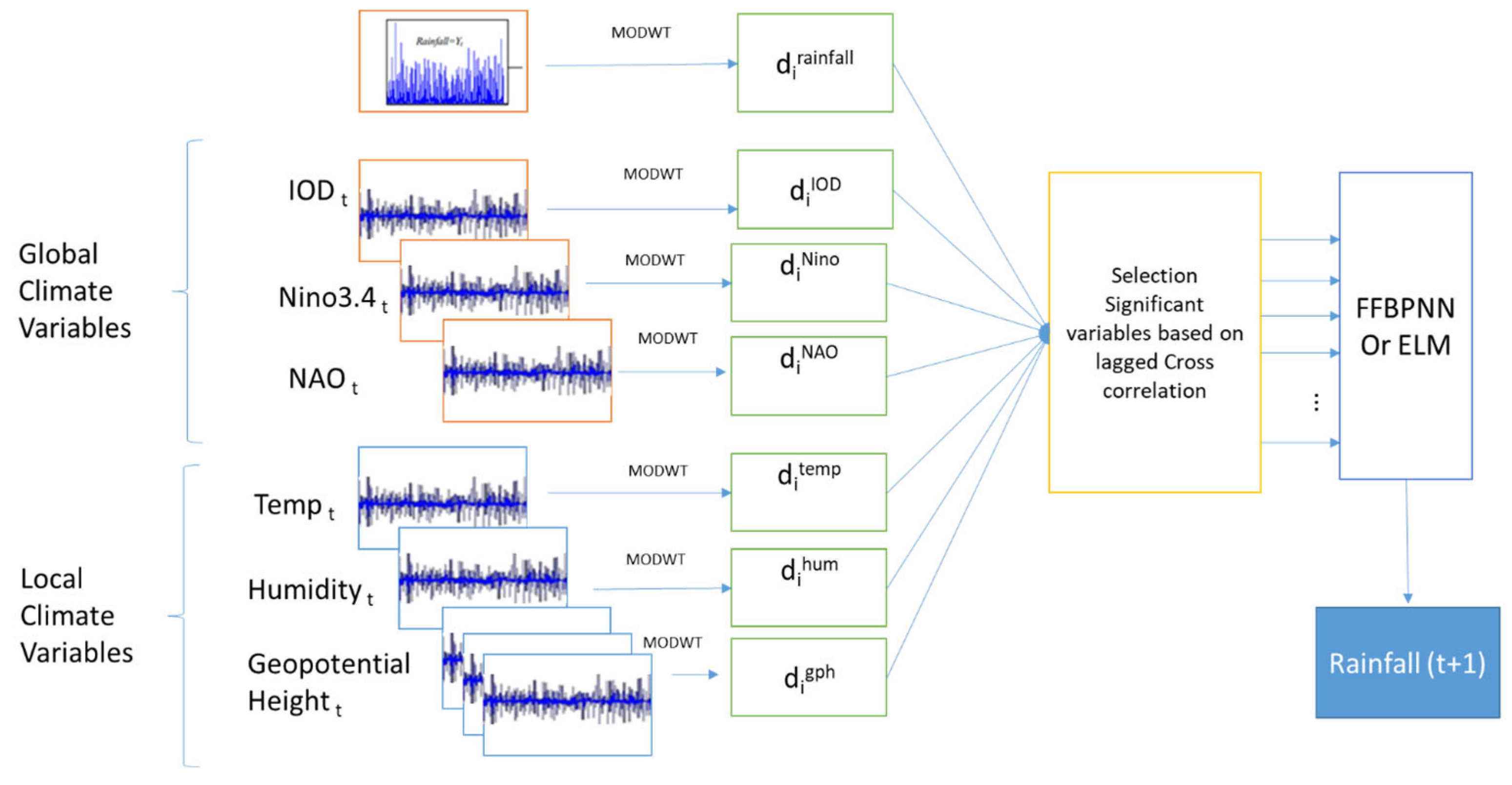
In wavelet hybrid models, the decomposed components of the original series and climate predictor variable are used to improve the quality of the precipitation forecast. As mentioned in Section 3.1, decomposition is carried out using a maximal overlap discrete wavelet transform (MODWT). The capability of wavelet models to identify hidden relationships among predictors and predictors by decomposition of the variables is the main advantage of using wavelet decomposition.
In this work, a feed-forward back-propagation neural network model (FFPBP-NN) based on previous literature and ELM models is coupled with wavelets to develop wavelet hybrid models. These models are denoted as WT-FFBP-NN and WT-ELM. A detailed description of FFBP-NN and multiple linear regression models is provided in Appendix A.1 and Appendix A.2.

4. Methodology

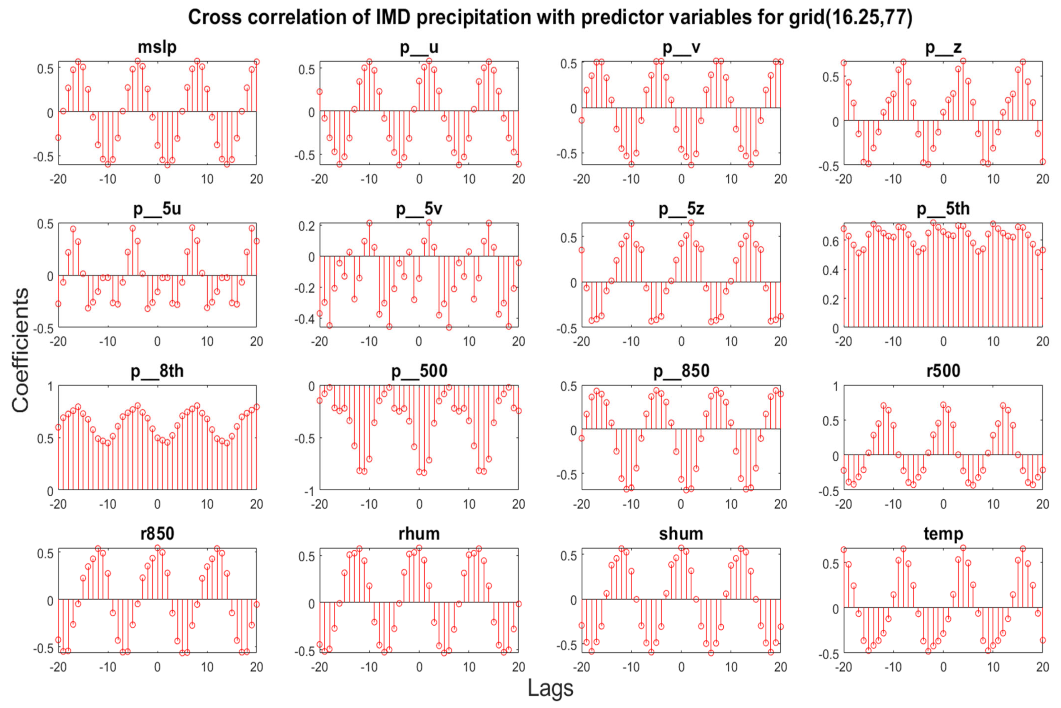
4.1. STEP: Identification of Significant Variables

Based on the literature, precipitation is assumed to respond to large-scale climate signals and local predictors with time lags. Auto correlation function (ACF) and cross-correlation function (CCF) are the lags at which the predictor variables influence precipitation. Based on CCF, the lag correlation of various predictor variables is determined and used to develop forecasting models.

4.2. STEP:1 Selection of Predictor Variables

After the first step, the climate predictor variables are chosen based on the values of correlation and cross-correlation function (CCF) to determine the predictor monthly and seasonal subseries of lag components with precipitation. Some of the sample correlation plots are shown in Figure 4. The correlation of climatic indices at different lag values is shown in Figure 4 at monthly scales to determine the lag component at which the indices are closely related to the precipitation time series.
It can be seen that each index has varying relationships with precipitation. Based on these values, the components of indices to be used in the analysis are selected [37]. These climatic indices and predictors are selected based on previous works [2,34,35,38] Also, along with the lagged values, zero lag coefficients are also used in the presence of long-term and short-term memory [39].

4.3. STEP 2 Standardization

After selecting predictor variables, the data sets are standardized to reduce the effect of the difference in magnitude between different variables. In this work, the standardization of variables is carried out using Equation (7)
x s t d = x x m i n x m a x x m i n
where x represents the predictor variables, x s t d = standardized value of predictor variables, x m i n and x m a x represent the minimum value and maximum value of predictor variable x .

4.4. Step 3: Model Development

4.4.1. Single-Scale Models (MLR, FFBP-NN, ELM)

After selecting probable predictors based on correlation and CCF of variables with monthly precipitation time series based on lag components, the entire data set is divided into 70:30 ratios. Training of the models is carried out using 70% of the data set, and validation of the models is carried out using the remaining 30% of the data. The performance of these models is evaluated using the performance measures mentioned in Section 4.4.3.

4.4.2. Wavelet Hybrid Models (WT-FFBP-NN and WT-ELM)

MODWT is applied to the predictor variables after selecting suitable potential predictors to decompose the data sets at various scales. As mentioned by [30], selecting suitable mother wavelets and levels of decomposition helps capture required features that provide information for good results. An optimum decomposition level and mother wavelet choice are selected based on [40] and [28,35] The lagged decomposed predictor variables are given as input for both WT-FFBP-NN and WT-ELM models.
The schematic of the methodology adopted for developing the wavelet-based hybrid models is shown in Figure 4. The different experiments generated by altering the methods and data used are tabulated in Table 2.

4.4.3. Performance Measures

This study verifies the accuracy and confidence limit of the model’s forecast using statistical metrics (Figure 5). The measures used in this study are root mean square error (RMSE), correlation (R2), Nash Sutcliffe efficiency (NSE), and most absolute error (MAE).
If the values of RMSE are high, the error component in the forecast to the original system is large, whereas if the values of NSE and correlation are nearer to 1, the obtained results are closer to the original system. If the values are nearer to 0, the model output is not a correct representation of the original system. RMSE and MAE represent the error component in the models.
  • Root Mean Square Error (RMSE)
    R M S E = 1 n i = 1 n ( X i o b s X i s i m ) 2   X   100 %
  • Correlation (R2)
    R 2 = i = 1 n x i o b s x m e a n o b s x i s i m x m e a n s i m i = 1 n x i o b s x m e a n o b s 2 x i s i m x m e a n s i m 2 2
  • Nash Sutcliffe Efficiency (NSE)
    N S E = 1 i = 1 n ( X i o b s X i s i m ) 2 i = 1 n ( X i o b s X i s i m m e a n ) 2
  • Most Absolute Error (MAE)
    MAE = i = 1 n | ( X i o b s X i s i m ) | n
    where X i o b s represents the ith observed data, X i s i m represents the simulated data from the models, X i m e a n is the mean of the data set, and n is the number of observations.

5. Results and Discussions

5.1. Forecasting Using Single Scale Models

The training and validation of all the models, including hybrid models such as wavelet hybrid models (WT-FFBP-NN and WT-ELM), were performed using performance measures (Section 4.4.3) until satisfactory results in terms of NSE and RMSE for precipitation forecasting were obtained. To test the efficacy of the models, five locations (one from each climate classification) in the Krishna River basin were selected to develop models and analyze precipitation in the basin.

5.2. For the Krishna River Basin

5.2.1. Results of the Models Using Only Global Climate Indices as Predictors

The results obtained from all the models using only the global climate indices and lagged precipitation data are shown in Table 3. The results show that MLR models obtained correlation values ranging from 0.30–0.37 and NSE values from 0.11 to 0.16. For FFBP-NN models, the forecast results showed correlation values ranging from 0.66–0.73 and NSE from 0.44 to 0.52. The results from the ELM model had a correlation ranging from 0.34–0.56 and NSE in the range of 0.34–0.51 for the five stations considered. WT-FFBP-NN model results yielded NSE values of 0.38–0.40 with a correlation of 0.56–0.64.
WT-ELM models showed an improved performance in terms of NSE and CC compared to the other models, as shown in Table 3.

5.2.2. Results of the Models Using Only Local Climate Variables as Predictors

Table 4 shows the results of the models for the Krishna River basin at all the selected locations at a monthly scale with only local predictors variables as inputs. The results show that the MLR model has correlation values ranging from 0.57 to 0.68 for the five locations, and the NSE values ranged between 0.32–0.40.
Comparative results were obtained using FFBP-NN and ELM models, where the NSE values ranged between 0.44–0.52 for the former and 0.43–0.50 for the latter, respectively. However, the results from WT-FFBP-NN and WT-ELM show higher values, with NSE values ranging between 0.50–0.56 and 0.51–0.57, respectively.

5.2.3. Results of Models with Both Global Climate Variables and Local Predictor Variables

In this case, local and global climate variables were considered along with the lagged precipitation for forecasting.
The results shown in Table 5 show a considerable increase in the model accuracy in terms of NSE, RMSE, and MAE. Further, it is also observed that the wavelet-based hybrid models, WT-FFBP-NN and WT-ELM, provided better forecasts than the other models. The best model was the WT-ELM, with the NSE ranging from 0.62–0.85 and the correlation coefficient in the range of 0.77–0.92.
It was also observed that the models using only global climate indices as inputs obtained the highest NSE value of 0.52, and the models using local predictor variables obtained the highest value of 0.67, whereas for the models with global climate and local predictor variables as inputs, the NSE values were increased to an average of 28% compared to those with only local predictor variables. Therefore, from the results for all the stations, the highest correlation was obtained for WT ELM for station 1 with a value of 0.92, followed by WT FFBP-NN with the highest NSE value of 0.85. Similarly, the best results for all the other stations were obtained for WT ELM models. Overall, the values NSE and correlation show that WT ELM outperformed WT FFBP-NN models and other singular models in precipitation forecasting for the Krishna River basin.
Overall, it was observed that including both the global and local predictors improved precipitation accuracy. It was also observed that the results based on the wavelet-based models were more accurate compared to the other singular models considered in the study. When these models were coupled with wavelets, the model could capture the nonlinearity, which helped the WT ELM models to capture all the necessary details and produce reliable precipitation forecasts.
Further comparing the model results obtained from WT-ELM and WT-FFBP-NN models, the WT-ELM based showed superior performance. It is clear that by coupling machine learning models with wavelets, the forecasting capabilities of the models have increased, with the results which registered low values when modeled with basic models being found to be improved with the usage of WT-based hybrid models for forecasting.

5.3. Model Application for the Different Regions in India

The best model was the WT-ELM model based on the results obtained for the Krishna River basin. So, to test the model results for the entire country and generalize the model performance, WT-ELM models were developed for the four chosen locations for each region categorized by IMD based on precipitation. The results for the selected locations are shown in Table 6.

5.4. Central India

The results from the models show that the correlation values found to be 0.90, 0.87, 0.92 and 0.87, with the NSE values being 0.81, 0.72, 0.85, 0.75 and the values of MAE showing that the error component in the forecast is relatively low as the value is nearer to zero. Also, the value of RMSE is less than 0.08 for all the stations.

5.5. North India

The results from the WT-ELM models show that the correlation values are 0.84, 0.88, 0.82, and 0.78 with NSE values of 0.70, 0.77, 0.68, and 0.54, along with low MAE and RMSE values. These low RMSE and RMSE indicate that the error component in the forecasting model is less.

5.6. Peninsular India

The correlation values from the results show that values are 0.84, 0.79, 0.92, and 0.87, respectively, for the four selected stations with NSE values of 0.66, 0.61, 0.85, and 0.76. The values of MAE were also found to be low, similar to the results of the remaining regions.

5.7. Northwest

The results indicate that the correlation values in these regions are 0.91, 0.88,0.76, and 0.83, with NSE values of 0.84, 0.74, 0.50, and 0.67.
Based on the results in Table 3, Table 4 and Table 5, the model that produced good results for all the different input combinations is the WT-ELM model with the highest correlation, highest NSE, and the lowest error component compared to the linear MLR model, machine learning models like FFBP-NN, ELM, and WT-FFBP-NN. Extending the analysis for the other grid locations, the models were applied to all the grid locations in the Indian subcontinent and the results are shown in Figure 6. It can be observed that the model results vary spatially and the best results are yielded using the WT-ELM compared to the other methods.

6. Discussion

In this study, wavelet-based hybrid models were tested for their ability to forecast monthly precipitation, and their performances were compared with those of some key traditional and other contemporary methods, including MLR, FFBP-NN, and ELM models. Among the different forecasting methods applied in this study, machine learning methods generally outperform the basic MLR models. Among the single-scale machine learning models, the ELM model outperformed the FFBP-NN model. The better performance of the ELM model may be due to its ability to capture the long- and short-term memory relationship between the climatic variables and precipitation.
Overall, our results manifest that the wavelet-based hybrid models (WT-FFBP-NN and WT-ELM) are accurate compared to the traditional and other machine-learning methods considered in this study. This observation is congruent with the broader understanding of the performance of the wavelet-based hybrid models, wherein wavelets enhance the models’ capability to unravel the multi-scale relationship among the variables. For example, in a recent study, [41] showed that wavelet-based decomposition helps identify the correlation between different variables, improving the model skill score. Similarly, in another study by [29], the authors showed that the wavelet-based models are accurate for streamflow forecasting. Another study, [42], showed that a wavelet based Volterra model performed superiorly to simple non-linear models for rainfall forecasting.
To understand the possible reasons for improving the performance of the wavelet-based models, see the correlations between the precipitation and climatic variables with and without wavelet decomposition. Table 6 shows the values of the same for Grid 2.
The correlation between precipitation and geopotential height (p850) is −0.06 without applying wavelet decomposition; conversely, the correlation is on the order of −0.47 to −0.16 between decompositions of p850 (D4 to D9), and precipitation varies from −0.17 to −0.39. A similar kind of correlation can also be observed for several other variables (e.g., uas, p500, mlp) as shown in Table 7. Overall, it is observed that there is a significant improvement in the correlation, or in other words, wavelets can unravel the hidden relationships and improve the performance of the forecasting models.
It is pertinent to understand that the NCEP reanalysis data have been used; however, the methodology can be extended to the weather forecasting model results and used to extend the forecast lead time.

7. Conclusions

The aim of this study is to develop a precipitation-forecasting model at monthly time scale considering the local and global climate predictors. For this purpose, a hybrid model was developed using wavelets and extreme learning models. The developed method was compared with other methods like multiple linear regression models, artificial neural networks, and wavelet neural networks through a case study in predicting monthly precipitation for the Krishna River basin. Based on the results obtained from evaluation measures, the model with the best prediction capability was found, and its ability to capture extreme events was identified. The performance measures showed that WT ELM models captured the events with higher precision than WT FBP-NN models, with lower RMSE and higher NSE values. The developed model can be applied for forecasting precipitation at monthly and seasonal scale and can be used in water-resource-management and reservoir-operation policy. The outcome of this study indicates the capability of WT ELM models to forecast precipitation, and their applicability can be understood from the results from the case study for the Krishna river basin.

Author Contributions

Conceptualization, M.R. and P.K.Y.; methodology, M.R., P.K.Y. and G.S.A.; software, G.S.A. and P.K.Y.; validation M.R., P.K.Y. and G.S.A.; formal analysis, S.S.S.N.; investigation, S.S.S.N. and G.S.A.; resources, S.S.S.N., G.S.A. and P.K.Y.; data curation, P.K.Y., G.S.A. and S.S.S.N.; writing—original draft preparation, P.K.Y., G.S.A. and S.S.S.N.; writing—review and editing, M.R.; visualization, P.K.Y. and S.S.S.N.; supervision, M.R.; project administration, M.R.; funding acquisition, M.R. All authors have read and agreed to the published version of the manuscript.

Funding

This research was funded by the name of IIT H, grant number SEED GRANT/SG114.

Data Availability Statement

The data used in this study can be made available from the sources mentioned in the manuscript.

Acknowledgments

R.M. gratefully acknowledges the SEED Grant (SG-114) funding from IIT Hyderabad, India.

Conflicts of Interest

The authors declare no conflict of interest.

Appendix A

Appendix A.1. Multiple Learning Regression (MLR)

Multiple linear regression is a form of linear regression analysis which develops the relationship between multiple predictor variables ( x 1 , x 2 , x 3 , . x n ) with respect to predictand variable (y) and this relationship can be understood using Equation (A1).
y = a 1 + a 2 x 1 + a 2 . a n x n
where a 1 , a 2 , a 3 . a n are calculated using the simple least squares method. A detailed explanation of the MLR model can be understood by referring to [43].

Appendix A.2. Artificial Neural Networks (ANN)

Artificial Neural Networks are defined as signal processing using neurons that save required experimental data to use for other processes. ANN has been developed to resemble the biological nervous system and it learns, stores, and processes data sets based on examples. Understanding complex relationships between inputs and targets, which is impossible using linear algorithms, can be performed easily and accurately using ANNs [44]. ANNs have been used for a few decades in various fields to analyze different kinds of problems in hydrology and climatology. The application of this method can be further understood by seeing works like [30,45,46,47,48,49]. The ability of ANNs to learn and simulate the results based on the provided inputs show its capability to solve complex problems that linear models cannot [50]. Further, the structure and capabilities of ANNs can be understood in detail by referring to [42,51,52]. While training a network, the number of neurons is varied numerous times using the trial-and-error method until the satisfaction of minimum-criteria error [42]. Numerous training functions are available for training neural networks to understand and capture input–output relationships. Some of the functions are the feed-forward back propagation neural network (FFBP-NN), non-linear auto regressive with exogenous inputs neural network (NARX-NN), and generalized regression neural network (GRNN). In this work, for the application of models, FFBP-NN models were used for forecasting precipitation due to their higher applicability than other models. For a detailed understanding of this model, readers can refer to [53,54], among others.
The FFBP-NN is a multiple-layer network consisting of neurons that are stacked in layers and connected with each other. Inputs and outputs of the networks are the first and last layers of the networks, with hidden layers being the remaining layers that carry information in the form of weights. In this study, FFBP-NN is trained, which is most widely used, especially in hydrologic applications. In this model, input data in the layers are given by x 1 , x 2 , x 3 . x n and the results from the output layer are given as y 1 , y 2 , y 3 . y n . The input neurons are connected with hidden layers by the weights, which connect the tth and the kth neurons, represented by w t k , whereas w j t represents the connection between hidden layers and the outputs layer. Being non-linear functions, ANNs capture the relationship between the input and output layer and the correlation for output can be understood [55] by Equation (A2)
y j = f o t = 1 s w j t . f h t = 1 s w t k x k + b t + b j
where f o and f h denote the activation function in the output layer and the activation function of nodes in the hidden layer. b t and b j are bias of tth neuron and jth neuron. s   and   s represent the nodes in the input and hidden layer, respectively.
The training algorithm used in the developing of the FFBP-NN model is Levenberg–Marquardt (LM), which is assumed to be one of the fastest and most accurate due to its recurrence to incorporate experience in training processes [36].

References

  1. Trenberth, K.E.; Smith, L.; Qian, T.; Dai, A.; Fasullo, J. Estimates of the Global Water Budget and Its Annual Cycle Using Observational and Model Data. J. Hydrometeorol. 2007, 8, 758–769. [Google Scholar] [CrossRef]
  2. Elahi, E.; Khalid, Z.; Tauni, M.Z.; Zhang, H.; Lirong, X. Extreme weather events risk to crop-production and the adaptation of innovative management strategies to mitigate the risk: A retrospective survey of rural Punjab, Pakistan. Technovation 2022, 117, 102255. [Google Scholar] [CrossRef]
  3. Wijeratne, V.P.I.S.; Li, G.; Mehmood, M.S.; Abbas, A. Assessing the Impact of Long-Term ENSO, SST, and IOD Dynamics on Extreme Hydrological Events (EHEs) in the Kelani River Basin (KRB), Sri Lanka. Atmosphere 2023, 14, 79. [Google Scholar] [CrossRef]
  4. Maheswaran, R.; Khosa, R. A Wavelet-Based Second Order Nonlinear Model for Forecasting Monthly Rainfall. Water Resour. Manag. 2014, 28, 5411–5431. [Google Scholar] [CrossRef]
  5. Yilmaz, A.G.; Muttil, N. Runoff Estimation by Machine Learning Methods and Application to the Euphrates Basin in Turkey. J. Hydrol. Eng. 2014, 19, 1015–1025. [Google Scholar] [CrossRef]
  6. Feng, G.-L.; Yang, J.; Zhi, R.; Zhao, J.-H.; Gong, Z.-Q.; Zheng, Z.-H.; Xiong, K.-G.; Qiao, S.-B.; Yan, Z.; Wu, Y.-P.; et al. Improved prediction model for flood-season rainfall based on a nonlinear dynamics-statistic combined method. Chaos Solitons Fractals 2020, 140, 110160. [Google Scholar] [CrossRef]
  7. Cuo, L.; Pagano, T.C.; Wang, Q.J. A Review of Quantitative Precipitation Forecasts and Their Use in Short- to Medium-Range Streamflow Forecasting. J. Hydrometeorol. 2011, 12, 713–728. [Google Scholar] [CrossRef]
  8. Hao, Z.; Singh, V.P.; Xia, Y. Seasonal Drought Prediction: Advances, Challenges, and Future Prospects. Rev. Geophys. 2018, 56, 108–141. [Google Scholar] [CrossRef]
  9. Bauer, H.-S.; Schwitalla, T.; Wulfmeyer, V.; Bakhshaii, A.; Ehret, U.; Neuper, M.; Caumont, O. Quantitative precipitation estimation based on high-resolution numerical weather prediction and data assimilation with WRF—A performance test. Tellus Ser. A Dyn. Meteorol. Oceanogr. 2015, 67, 25047. [Google Scholar] [CrossRef]
  10. Stensrud, D.J.; Xue, M.; Wicker, L.J.; Kelleher, K.E.; Foster, M.P.; Schaefer, J.T.; Schneider, R.S.; Benjamin, S.G.; Weygandt, S.S.; Ferree, J.T.; et al. Convective-scale warn-on-forecast system: A vision for 2020. Bull. Am. Meteorol. Soc. 2009, 90, 1487–1500. [Google Scholar] [CrossRef]
  11. Saha, S.K.; Pokhrel, S.; Chaudhari, H.S.; Dhakate, A.; Shewale, S.; Sabeerali, C.T.; Salunke, K.; Hazra, A.; Mahapatra, S.; Rao, A.S. Improved simulation of Indian summer monsoon in latest NCEP climate forecast system free run. Int. J. Climatol. 2013, 34, 1628–1641. [Google Scholar] [CrossRef]
  12. Molteni, F.; Buizza, R.; Palmer, T.N.; Petroliagis, T. The ECMWF Ensemble Prediction System: Methodology and validation. Q. J. R. Meteorol. Soc. 1996, 122, 73–119. [Google Scholar] [CrossRef]
  13. Choubin, B.; Khalighi-Sigaroodi, S.; Malekian, A.; Kişi, Ö. Multiple linear regression, multi-layer perceptron network and adaptive neuro-fuzzy inference system for forecasting precipitation based on large-scale climate signals. Hydrol. Sci. J. 2016, 61, 1001–1009. [Google Scholar] [CrossRef]
  14. Xu, L.; Chen, N.; Zhang, X.; Chen, Z. An evaluation of statistical, NMME and hybrid models for drought prediction in China. J. Hydrol. 2018, 566, 235–249. [Google Scholar] [CrossRef]
  15. Ghamariadyan, M.; Imteaz, M.A. A wavelet artificial neural network method for medium-term rainfall prediction in Queensland (Australia) and the comparisons with conventional methods. Int. J. Climatol. 2021, 41, E1396–E1416. [Google Scholar] [CrossRef]
  16. Chowdhury, R.K.; Beecham, S. Australian rainfall trends and their relation to the southern oscillation index. Hydrol. Process 2010, 24, 504–514. [Google Scholar] [CrossRef]
  17. Abbot, J.; Marohasy, J. Application of artificial neural networks to rainfall forecasting in Queensland, Australia. Adv. Atmos. Sci. 2012, 29, 717–730. [Google Scholar] [CrossRef]
  18. Rivera, D.; Lillo, M.; Uvo, C.B.; Billib, M.; Arumí, J.L. Forecasting monthly precipitation in Central Chile: A self-organizing map approach using filtered sea surface temperature. Theor. Appl. Climatol. 2012, 107, 1–13. [Google Scholar] [CrossRef]
  19. Barzegar, R.; Moghaddam, A.A.; Adamowski, J.; Ozga-Zielinski, B. Multi-step water quality forecasting using a boosting ensemble multi-wavelet extreme learning machine model. Stoch. Environ. Res. Risk Assess. 2018, 32, 799–813. [Google Scholar] [CrossRef]
  20. Alizamir, M.; Kisi, O.; Zounemat-Kermani, M. Modelling long-term groundwater fluctuations by extreme learning machine using hydro-climatic data. Hydrol. Sci. J. 2017, 63, 63–73. [Google Scholar] [CrossRef]
  21. Li, B.; Cheng, C. Monthly discharge forecasting using wavelet neural networks with extreme learning machine. Sci. China Technol. Sci. 2014, 57, 2441–2452. [Google Scholar] [CrossRef]
  22. Ummenhofer, C.C.; Gupta, A.S.; England, M.H.; Reason, C.J.C. Contributions of Indian Ocean Sea Surface Temperatures to Enhanced East African Rainfall. J. Clim. 2009, 22, 993–1013. [Google Scholar] [CrossRef]
  23. Rathinasamy, M.; Agarwal, A.; Sivakumar, B.; Marwan, N.; Kurths, J. Wavelet analysis of precipitation extremes over India and teleconnections to climate indices. Stoch. Stoch. Environ. Res. Risk Assess. 2019, 33, 2053–2069. [Google Scholar] [CrossRef]
  24. Daubechies, I. The wavelet transform, time-frequency localization and signal analysis. IEEE Trans. Inf. Theory 1990, 36, 961–1005. [Google Scholar] [CrossRef]
  25. Küçük, M.; Tigli, E.; Ağiralioğlu, N. Wavelet Transform Analysis for Nonstationary Rainfall-Runoff-Temperature Processes. 2004. Available online: http://www.r-project.org (accessed on 22 June 2023).
  26. Park, J.; Mann, M.E. Paper No. 1 • Page 1 Copyright. 2000. Available online: http://earthinteractions.org (accessed on 22 June 2023).
  27. Grossmann; Morlet, J. Decomposition of Hardy Functions into Square Integrable Wavelets of Constant Shape*. 1984. Available online: https://epubs.siam.org/terms-privacy (accessed on 22 June 2023).
  28. Renaud, O.; Starck, J.-L.; Murtagh, F. Wavelet-Based Combined Signal Filtering and Prediction. IEEE Trans. Syst. Man Cybern. Part B Cybern. 2005, 35, 1241–1251. [Google Scholar] [CrossRef] [PubMed]
  29. Adamowski, J.; Sun, K. Development of a coupled wavelet transform and neural network method for flow forecasting of non-perennial rivers in semi-arid watersheds. J. Hydrol. 2010, 390, 85–91. [Google Scholar] [CrossRef]
  30. Maheswaran, R.; Khosa, R. Comparative study of different wavelets for hydrologic forecasting. Comput. Geosci. 2012, 46, 284–295. [Google Scholar] [CrossRef]
  31. Huang, G.-B.; Zhu, Q.-Y.; Siew, C.-K. Extreme learning machine: Theory and applications. Neurocomputing 2006, 70, 489–501. [Google Scholar] [CrossRef]
  32. Huang, G.-B. What are Extreme Learning Machines? Filling the Gap Between Frank Rosenblatt’s Dream and John von Neumann’s Puzzle. Cognit. Comput. 2015, 7, 263–278. [Google Scholar] [CrossRef]
  33. Yaseen, Z.M.; Jaafar, O.; Deo, R.C.; Kisi, O.; Adamowski, J.; Quilty, J.; El-Shafie, A. Stream-flow forecasting using extreme learning machines: A case study in a semi-arid region in Iraq. J. Hydrol. 2016, 542, 603–614. [Google Scholar] [CrossRef]
  34. Deo, R.C.; Şahin, M. An extreme learning machine model for the simulation of monthly mean streamflow water level in eastern Queensland. Environ. Monit. Assess. 2016, 188, 1–24. [Google Scholar] [CrossRef]
  35. Deo, R.C.; Şahin, M. Application of the Artificial Neural Network model for prediction of monthly Standardized Precipitation and Evapotranspiration Index using hydrometeorological parameters and climate indices in eastern Australia. Atmos. Res. 2015, 161–162, 65–81. [Google Scholar] [CrossRef]
  36. Swapna, P.; Roxy, M.K.; Aparna, K.; Kulkarni, K.; Prajeesh, A.G.; Ashok, K.; Krishnan, R.; Moorthi, S.; Kumar, A.; Goswami, B.N. The IITM Earth System Model: Transformation of a Seasonal Prediction Model to a Long-Term Climate Model. Bull. Am. Meteorol. Soc. 2015, 96, 1351–1367. [Google Scholar] [CrossRef]
  37. Ren, H.-L.; Lu, B.; Wan, J.; Tian, B.; Zhang, P. Identification Standard for ENSO Events and Its Application to Climate Monitoring and Prediction in China. J. Meteorol. Res. 2018, 32, 923–936. [Google Scholar] [CrossRef]
  38. Sehgal, V.; Lakhanpal, A.; Maheswaran, R.; Khosa, R.; Sridhar, V. Application of multi-scale wavelet entropy and multi-resolution Volterra models for climatic downscaling. J. Hydrol. 2018, 556, 1078–1095. [Google Scholar] [CrossRef]
  39. Kannan, S.; Ghosh, S. Prediction of daily rainfall state in a river basin using statistical downscaling from GCM output. Stoch. Environ. Res. Risk Assess. 2011, 25, 457–474. [Google Scholar] [CrossRef]
  40. Lakhanpal, A.; Sehgal, V.; Maheswaran, R.; Khosa, R.; Sridhar, V. A non-linear and non-stationary perspective for downscaling mean monthly temperature: A wavelet coupled second order Volterra model. Stoch. Environ. Res. Risk Assess. 2017, 31, 2159–2181. [Google Scholar] [CrossRef]
  41. Kumar, Y.P.; Maheswaran, R.; Agarwal, A.; Sivakumar, B. Intercomparison of downscaling methods for daily precipitation with emphasis on wavelet-based hybrid models. J. Hydrol. 2021, 599, 126373. [Google Scholar] [CrossRef]
  42. Maheswaran, R.; Khosa, R. Wavelet Volterra Coupled Models for forecasting of nonlinear and non-stationary time series. Neurocomputing 2015, 149, 1074–1084. [Google Scholar] [CrossRef]
  43. Olive, D.J. Prediction intervals for regression models. Comput. Stat. Data Anal. 2006, 51, 3115–3122. [Google Scholar] [CrossRef]
  44. Alizadeh, M.J.; Kavianpour, M.R.; Kisi, O.; Nourani, V. A new approach for simulating and forecasting the rainfall-runoff process within the next two months. J. Hydrol. 2017, 548, 588–597. [Google Scholar] [CrossRef]
  45. Kişi, Ö. Neural Networks and Wavelet Conjunction Model for Intermittent Streamflow Forecasting. J. Hydrol. Eng. 2009, 14, 773–782. [Google Scholar] [CrossRef]
  46. Nourani, V.; Komasi, M.; Mano, A. A Multivariate ANN-Wavelet Approach for Rainfall–Runoff Modeling. Water Resour. Manag. 2009, 23, 2877–2894. [Google Scholar] [CrossRef]
  47. Okkan, U.; Fistikoglu, O. Evaluating climate change effects on runoff by statistical downscaling and hydrological model GR2M. Theor. Appl. Climatol. 2013, 117, 343–361. [Google Scholar] [CrossRef]
  48. Ahmed, B.; Al Noman, A. Land cover classification for satellite images based on normalization technique and Artificial Neural Network. In Proceedings of the 2015 International Conference on Computer and Information Engineering (ICCIE), Rajshahi, Bangladesh, 26–27 November 2015; pp. 138–141. [Google Scholar] [CrossRef]
  49. Vu, M.T.; Aribarg, T.; Supratid, S.; Raghavan, S.V.; Liong, S.-Y. Statistical downscaling rainfall using artificial neural network: Significantly wetter Bangkok? Theor. Appl. Climatol. 2015, 126, 453–467. [Google Scholar] [CrossRef]
  50. Rumelhart, D.E.; Widrow, B.; Lehr, M.A. The basic ideas in neural networks. Commun. ACM 1994, 37, 87–92. [Google Scholar] [CrossRef]
  51. Kuligowski, R.J.; Barros, A.P. Localized Precipitation Forecasts from a Numerical Weather Prediction Model Using Artificial Neural Networks. Weather Forecast. 1998, 13, 1194–1204. [Google Scholar] [CrossRef]
  52. Tokar, A.S.; Markus, M. Precipitation-Runoff Modeling Using Artificial Neural Networks and Conceptual Models. J. Hydrol. Eng. 2000, 5, 156–161. [Google Scholar] [CrossRef]
  53. Haykin, S. Neural Networks and Learning Machines; Pearson: London, UK, 2008; Volume 3, ISBN 978-0131471399. [Google Scholar]
  54. Shanmuganathan, S. Studies in Computational Intelligence 628 Artificial Neural Network Modelling; Springer: Berlin/Heidelberg, Germany, 2016; Volume 628, Available online: http://www.springer.com/series/7092 (accessed on 22 June 2023).
  55. Santos, C.A.G.; Kisi, O.; da Silva, R.M.; Zounemat-Kermani, M. Wavelet-based variability on streamflow at 40-year timescale in the Black Sea region of Turkey. Arab. J. Geosci. 2018, 11, 169. [Google Scholar] [CrossRef]
Figure 1. Koeppen climate classification for India. The Koeppen climate classification scheme divides climates into five main climate groups: A (tropical), B (arid), C (temperate), D (continental), and E (polar). The first letter indicates the climate groups. The second letter indicates the seasonal precipitation type, while the third letter indicates the level of heat. The detailed explanation of the abbreviation is provided in https://www.mindat.org/climate.php accessed on 30 August 2022.
Water 15 03244 g001
Figure 2. (a) Geographical location of selected stations in the Krishna River basin. (b). Precipitation variability map and DEM of the Krishna River basin.
Water 15 03244 g002
Figure 3. Schematic representation of extreme learning machines.
Water 15 03244 g003
Figure 4. Schematic of the methodology used in developing the wavelet-based model for precipitation forecasting. The time scale of the variables considered is a monthly time scale.
Water 15 03244 g004
Figure 5. Sample cross-correlation between different predictors and precipitation for Grid 2 (16.25N, 77E).
Water 15 03244 g005
Figure 6. Spatial map of NSE for various models for India using (a) FFBP—NN, (b) ELM, (c) WT FFBP—NN, and (d) WT—ELM models.
Water 15 03244 g006
Table 1. Details of global and local predictor variables used for precipitation forecasting.
LevelPredictands
GlobalIndian Oceanic Dipole (IOD)
North Atlantic Oscillation (NAO)
NINO
Pacific Decadal Oscillation (PDO)
LocalMean Sea level pressure (mslp)
Zonal velocity component (p_u)
Meridional velocity component (p_v)
Vorticity (p_z)
Specific humidity (shum)
Relative humidity (rhum)
Surface air temperature (temp)
Zonal velocity component (p5_u)
Meridional velocity component (p5_v)
Vorticity (p5_z)
Wind direction (p5th)
Geopotential height (p500)
Relative humidity (r500) Wind direction (p8th)
Geopotential height (p850)
Relative humidity (r850)
Table 2. Prediction experiment using different input combination and modelling methods.
ModelsInputWavelet TransformOutput
Single-Scale Models (FFBP-NN, ELM, MLR)Lagged Precipitation and Global TeleconnectionNoPrecipitation at t + 1
Single-Scale Models (FFBP-NN, ELM, MLR)Lagged Precipitation and Local Climate VariablesNoPrecipitation at t + 1
Single-Scale Models (FFBP-NN, ELM, MLR)Lagged Precipitation and Global Teleconnection+ Local Climate VariablesNoPrecipitation at t + 1
Multi-Scale Models (FFBP-NN, ELM, MLR)Lagged Precipitation and Global TeleconnectionYesPrecipitation at t + 1
Multi-Scale Models (FFBP-NN, ELM, MLR)Lagged Precipitation and Local Climate VariablesYesPrecipitation at t + 1
Multi-Scale Models (FFBP-NN, ELM, MLR)Lagged Precipitation and Global Teleconnection + Local Climate VariablesYesPrecipitation at t + 1
Table 3. Results for various forecasting models for the Krishna River basin with global climate indices as inputs. The values for RMSE and MAE are normalized with respect to mean and standard deviation.
StationMLR
RMSE (mm)CorrelationNSEMAE (mm)
10.0960.3550.1640.099
20.1600.3320.1240.100
30.1620.3760.1370.105
40.1440.3090.1570.092
50.0480.3090.1190.055
FFBP-NN
10.0900.6940.4810.058
20.0910.6800.4580.063
30.0920.6690.4460.065
40.0630.7300.5290.032
50.0520.7130.5040.036
ELM
10.0700.4070.4070.053
20.1010.4890.4030.067
30.1570.3430.3430.117
40.1220.4190.4190.096
50.0520.5610.5150.037
WT FFBP-NN
10.1110.5980.3850.077
20.1060.6440.4030.075
30.1130.5720.3850.078
40.1130.5670.3910.078
50.1080.6360.3830.080
WT ELM
10.0930.7850.4940.064
20.0880.8030.4520.063
30.1250.8120.4180.088
40.0960.7980.4650.063
50.1130.8480.4340.076
Table 4. Results for various forecasting models for the Krishna River basin with local predictor variables as inputs. The values for RMSE and MAE are normalized with respect to mean and standard deviation.
StationMLR
RMSE (mm)CorrelationNSEMAE (mm)
10.0530.5730.5730.037
20.0910.5360.5360.057
30.1230.5970.5970.084
40.0960.6460.6460.063
50.0580.4420.4420.033
FFBP-NN
10.0550.5450.5450.038
20.0860.5760.5760.054
30.0120.6000.6000.078
40.0920.6780.6780.058
50.0620.7130.3620.031
ELM
10.0660.4730.4730.039
20.0940.4960.4960.060
30.1270.5650.5650.089
40.0940.6530.6530.062
50.0570.4230.4230.032
WT FFBP-NN
10.1090.7710.5560.069
20.0820.7790.5490.057
30.0840.7530.5050.063
40.0610.7870.5630.041
50.0700.7650.5200.052
WT ELM
10.1180.7790.5750.087
20.0860.7650.5570.065
30.0780.8170.5790.054
40.0750.7380.5180.056
50.0840.7420.5180.063
Table 5. Results for various forecasting models for the Krishna River basin with global climate and local variables as inputs. The values for RMSE and MAE are normalized with respect to mean and standard deviation.
StationMLR
RMSE (mm)CorrelationNSEMAE (mm)
10.0530.5780.3340840.037
20.090.5330.2840890.057
30.1220.6020.3624040.084
40.0960.6530.4264090.063
50.0590.4390.1927210.034
FFBP-NN
10.050.6160.3794560.035
20.0830.6040.3648160.049
30.1080.6910.4774810.069
40.0870.7140.5097960.053
50.0520.560.31360.032
ELM
10.0510.680.46240.034
20.0650.7570.5730490.042
30.090.7840.6146560.064
40.0750.7820.6115240.047
50.0370.7540.5685160.026
WT FFBP-NN
10.0330.8920.7956640.055
20.0720.8490.7208010.052
30.0770.7840.6146560.056
40.0610.8020.6432040.036
50.0440.820.67240.022
WT ELM
10.030.9250.8556250.052
20.0690.8430.7106490.053
30.0750.8130.6609690.058
40.0530.8470.7174090.035
50.0330.7790.6068410.013
Table 6. Results of WT ELM models for India with combined global and local predictor variables. The values for RMSE and MAE are normalized with respect to mean and standard deviation.
StationCentral India
RMSE (mm)CorrelationNSEMAE (mm)
10.07180.90840.81520.0059
20.06800.87510.72000.0491
30.07570.92600.85380.0584
40.07550.87750.75740.0567
North India
10.07330.84370.70120.0537
20.06100.88640.77330.0447
30.08000.82860.68160.0581
40.07280.78040.54770.0554
Peninsular
10.09270.84060.66190.0686
20.10090.79360.61120.0780
30.04190.93240.85800.0325
40.10300.87280.76020.0781
Northwest
10.07840.91780.84010.0603
20.06280.88730.74370.0448
30.08020.76110.50250.0578
40.06960.83560.67650.0532
Table 7. Correlation between different climatic variables and precipitation with and without wavelet decomposition for Grid 2 (Dn indicates the decomposition and its level).
Climatic VariableOriginal ScaleD1D2D3D4D5D6D7D8D9D10
p5zas0.0110.0110.0510.0610.0610.0810.1610.3610.4210.2710.121
p5th0.1310.001−0.009−0.019−0.059−0.069−0.0790.0010.3610.1410.081
p8th−0.0190.0010.0010.0110.001−0.029−0.159−0.369−0.409−0.329−0.109
rhum0.1110.0210.0310.0610.1210.2010.3310.4010.3610.3310.171
shum0.1410.0110.0310.0510.1010.1710.3210.4210.4110.3710.161
temp0.071−0.009−0.019−0.049−0.099−0.159−0.199−0.1290.0510.0110.021
mslp−0.079−0.039−0.079−0.139−0.169−0.149−0.239−0.349−0.389−0.349−0.099
uas0.0210.0210.0410.0810.1510.1910.2910.4310.4010.3710.091
vas−0.0290.0210.0410.0610.0710.0810.031−0.269−0.399−0.319−0.139
zas0.1710.0110.2210.0210.0210.0210.0010.0210.0710.0410.031
p5 uas−0.1590.0110.0210.0310.0610.0810.061−0.029−0.379−0.179−0.089
p5 vas0.0210.0210.0310.0210.001−0.019−0.019−0.109−0.269−0.089−0.009
p5000.091−0.029−0.069−0.119−0.149−0.159−0.209−0.289−0.369−0.119−0.009
p850−0.059−0.039−0.089−0.159−0.199−0.209−0.359−0.469−0.439−0.379−0.089
r5000.1010.0110.0410.0710.1110.1810.3110.4310.4210.3710.121
r8500.0510.0210.0410.0710.1410.2110.3210.4110.3510.3010.141
Note(s): Values in bold show a significant correlation at 95% confidence levels.
Disclaimer/Publisher’s Note: The statements, opinions and data contained in all publications are solely those of the individual author(s) and contributor(s) and not of MDPI and/or the editor(s). MDPI and/or the editor(s) disclaim responsibility for any injury to people or property resulting from any ideas, methods, instructions or products referred to in the content.

