Abstract
This modeling study intended to solve a part of the global scientific problem related to increased concentrations of carbon dioxide in the atmosphere via emissions from terrestrial ecosystems that, along with anthropogenic emissions, make notable contributions to the processes of climate change on the planet. The main stream of CO2 from natural terrestrial ecosystems is related to the activation of biological processes, such as the production/destruction of plant biomass. In this study, the Wetland-DNDC computer simulation model with a focus on nitrogen and carbon biogeochemical cycles was used to study the effect of hydrothermal conditions on greenhouse gas fluxes in West Siberian peatlands. The study was implemented on the site of the world’s largest pristine wetland/peatland system, the Great Vasyugan Mire (GVM). The study was carried out based on data from permanent measurements at meteo stations and our own in situ measurements of hydrological and thermal parameters on sites, which allowed for testing different scenarios of changes in environmental conditions (temperature, precipitation, groundwater level) together with a change in GHG fluxes. The study revealed the air temperature and the level of groundwater as the main drivers controlling CO2 fluxes. The study of different scenarios of change in annual air temperature revealed the threshold of change in the wetland/peatland ecosystem from carbon sink to carbon source to the atmosphere to happen with an increase in the average annual air temperature by 3 °C with reference to the average annual air temperature values in 2019. Also, we found that the wetland/peatland ecosystem turned to act as an active carbon sink with about 7 cm increase in annual groundwater level, compared with its base level of −21 cm.
1. Introduction
Wetland ecosystems are an important component of the terrestrial biosphere that specify the global carbon (C) cycle, and they define the way of climate change. The peat-accumulating wetlands (or so-called peatlands) represent 15 to 22% of terrestrial carbon stock at the global scale [1]. Basically, the carbon balance in the biosphere is a measure of two natural processes: (i) the accumulation of carbon through photosynthesis and (ii) the emissions of carbon dioxide (CO2) and methane (CH4) through the heterotrophic respiration and decomposition of organic matter. Wetland ecosystems have unique characteristics that affect carbon dynamics. Even small changes in groundwater level or temperature can change the carbon balance in peatlands to increase the rate of decomposition of soil organic matter and to increase the productivity of plant communities, or vice versa [2,3,4].
When building climate change scenarios based on simulation models, a wide range of factors constraining emissions of greenhouse gases (GHG) from soils should be taken into account, and these factors have been subject to great spatial and temporal variability [5,6]. Normally, the model performance is estimated by comparing emission data from direct in situ measurements with emissions data derived from the model run—the same way for environmental variables. This kind of modeling approach was used to estimate the set of all major parameters of the carbon cycle in different natural ecosystems (e.g., in wetlands and forests), at different geographic locations, and in different climatic conditions) as it is shown in some earlier studies [7,8,9,10]. There are a few simulation (ecosystem) models that have shown good performance in simulating natural processes in wetland ecosystems, which work with a range of climate change scenarios [11,12]. Wetland-DNDC [13,14,15,16] has the capability to predict CO2 and CH4 emissions under conditions of climate change, change hydrological conditions, and has various biogeochemical features of soils and for different vegetation (land cover types) [17].
The simplest scenarios in the Wetland-DNDC model take into account the ratio between single climatic variables and greenhouse gas fluxes. For instance, the study of Zhang et al. (2002) has found only slight temperature dependence on net primary production (NPP) for the wetlands in North America—a 12.4% decrease with a 2 °C temperature increase [13]. At the same time, for the Net Ecosystem Production (NEP) of forest ecosystems, the temperature remains the most important driver. The temperature was also shown as a strong driver of methane (CH4) fluxes [15,18]. A study of the alpine wetlands of the Qinghai-Tibet Plateau, where numerous sights of ongoing climate change have been lately observed, has shown that a marked increase in air temperatures in wintertime led to a notable increase in CO2 emissions [9].
The modeling study of Zhang et al. of the carbon dynamics in different scenarios of groundwater (WT) tables has revealed the highest annual CH4 emissions happened with a WT of 10 cm above the land surface [13]. A high correlation between net ecosystem exchange (NEE) and groundwater table was found in the peat bogs at the southern range of European taiga in Russia [18]. The high WTs imply the conditions for atmospheric carbon (CO2) sink, whereas the low WTs imply some increased rate of decomposition of plant organic matter (plant biomass), and ecosystems become carbon sources due to emissions of CO2 to the atmosphere. In particular, it was found with the Wetland-DNDC modeling study of the carbon exchange in the wetlands of Florida, USA. The lowering of the groundwater tables led to a decrease in CH4 emissions and an increase in CO2 emissions in the same ecosystems [19]. The same (Wetland-DNDC) model showed good performance in the study of greenhouse gas fluxes in wetlands of North America (Ontario, Canada) under contrast conditions of long-lasting floods and droughts [20]. The drought was found to drive increased CO2 fluxes and decreased CH4 fluxes. In contrast, the shallow floods led to a decrease in CO2 emissions and an increase in CH4 emissions.
Wetland-DNDC has shown high performance in a recent study of the Great Vasyugan Mire [16]. In this study, the most significant model input parameters were identified to estimate carbon fluxes and net ecosystem exchange (NEE), and it opens perspectives for use as a prognostic model with the set-up of different scenarios of climate change.
This work makes a focus on the use of the Wetland-DNDC model to estimate carbon fluxes at the site of pristine wetland/peatland in Western Siberia. It represents a small part of the Great Vasyugan Mire (a total area of 55,000 km2), which is the largest continuous wetland body on Earth. Our main hypothesis is that, similar to other studies, the level of groundwater could be the main driver of carbon fluxes at our test site. Then, one can predict the seasonal variations in groundwater levels under different climate change scenarios. It will further allow predictions of carbon fluxes between the mire landscapes and the atmosphere.
2. Materials and Methods
2.1. Materials
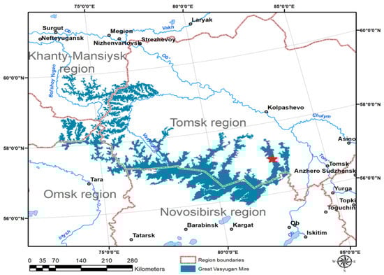
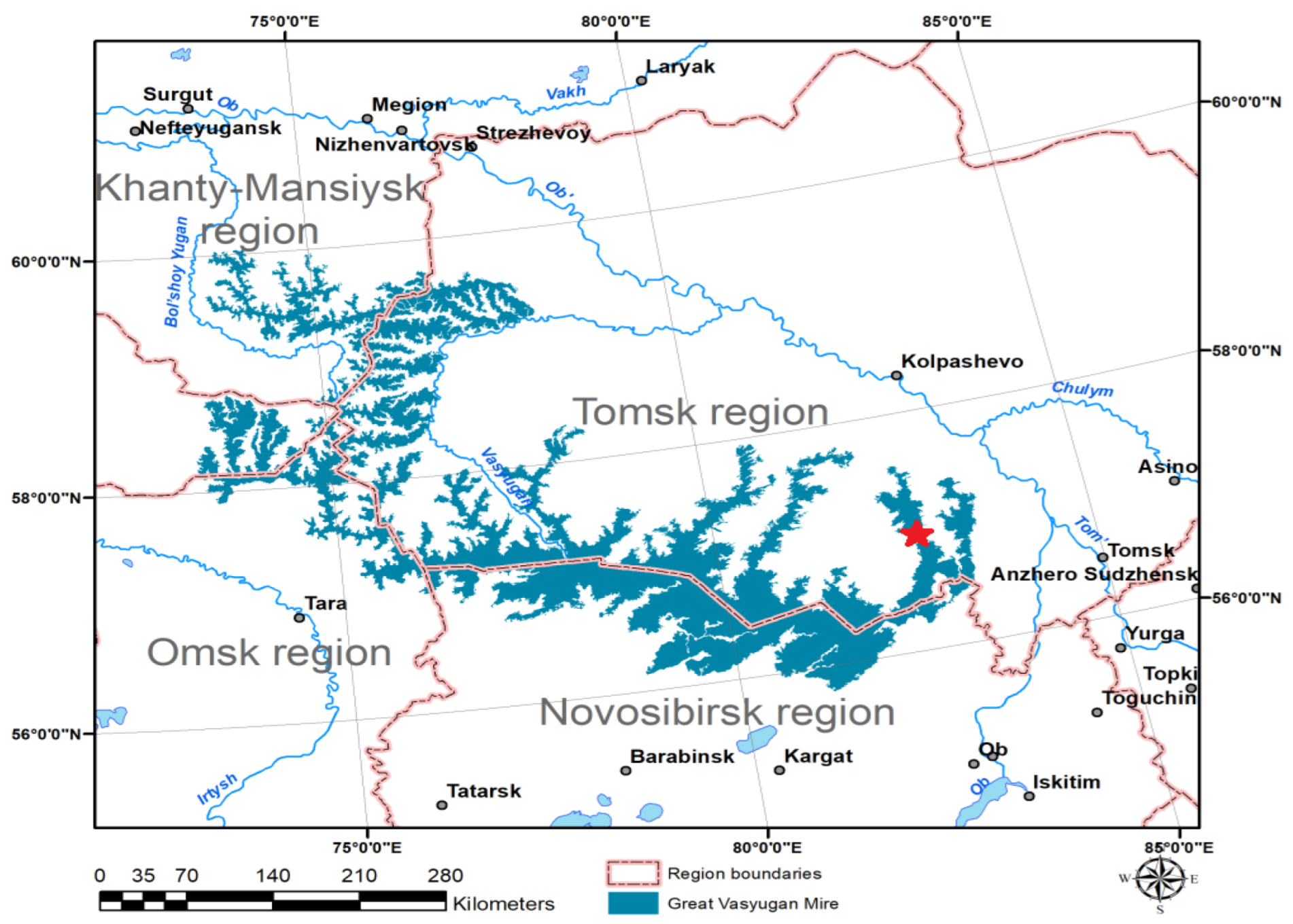
The studies were carried out at the part of the Great Vasyugan Mire (GVM)—the World’s largest peatland system—that is located in the southern taiga region of Western Siberia (WS) (Figure 1). The Great Vasyugan Mire represents a set of peat-accumulating ecosystems with a total area of 55,051 km2 [21], which was formed about 10,000 years ago by the confluence of different-sized individual mires, and the area is still under active formations [22]. At the study site (centered at N 56°58′24,3″, E 82°36′41.2″), the vegetation was presented by a pine-shrub-Sphagnum plant community. The tree layer dominated by pine (Pinus sylvestris) of up to 2 m in height makes a projective cover of 40%. The grass and shrub layer is dominated by 60% Chamaedaphne calyculata, 30% Ledum palustre, 10% Vaccinium uliginosum, Andromeda polifolia, and Eriophorum vaginatum—by 5% in the land cover, with single plants of Rubus chamaemorus. At the land surface, the Sphagnum mosses cover 95 to 100%, of which 80% is contributed by Sphagnum fuscum, with little presence of Sphagnum divinum and Sphagnum angustifolium. Some more details on the study site are presented in our earlier publication [16].
Figure 1.
Location of study site—The Great Vasyugan Mire (GVM). The red star is location of study site.
In situ measurements of CO2 fluxes were made by a chemical absorption method based on capturing CO2 emitted from a land surface with NaOH [23] once a month during the growing season (from 25 May to 17 October) in 2019. The measurements of CO2 fluxes were duplicated by a LI-7810SC (Li-COR Nebraska USA) gas analyzer. Normally, the absorption method underestimates the CO2 fluxes by 2.5 times, so the data of measurements were further corrected for bias [24]. The meteo data for the period of measurements were taken from the Bakchar weather station (available at http://meteo.ru/, URL accessed on 1 December 2022). The air temperature (T) and precipitation (P) were taken from meteo station Bakchar (located at a distance of 33 km from our study site; N 57°00′26.8″, E 82°03′34.3″), and the groundwater table was measured with the sensor system described in [25]. The solar radiation was measured directly on-site with a BISR solar radiation meter. The daily maximum and daily minimum air temperatures (Tmax and Tmin, °C, respectively), as well as precipitation (P, mm) and groundwater levels (WT, cm), were used as input model parameters.
A whole list of the model input values used to run the basic Wetland-DNDC simulation model is presented in the Appendix, Table A1. The initial set of hydrothermal parameters (Tmax and Tmin, P and WT, see Figure A1 in the Appendix) all have non-normal distributions according to the Shapiro–Wilk test. Therefore, in this study, we have used the non-parametric correlation coefficient of Spearman for statistical data analysis in the Statistica 10 software.
Statistical processing of the results from the Wetland-DNDC simulation model showed that the modeled hydrothermal factors (T, P, and WT) are not correlated with each other, and the model efficiency is high (R2 = 0.675)—as shown in the earlier publication [16]—therefore, our next target was a computer simulation of different hydrothermal scenarios and estimation of greenhouse gas fluxes under the change of these hydrothermal parameters (T, P, and WT).
2.2. Wetland-DNDC Model Description
In this study, we have used the Wetland-DNDC computer simulation model [14] to estimate ecosystem carbon exchange and greenhouse gas emissions, including methane (CH4), nitrous oxide (N2O), nitric oxide (NO), nitrogen (N2), and ammonia (NH3).
The Wetland-DNDC model takes into account a whole set of environmental variables (Table A1) to produce an integrated assessment of ecosystem carbon exchange—among them are the climate, hydrology, vegetation/land cover type, and soil type [26,27,28,29,30]. The model makes the links between C and N biogeochemical cycles and all major environmental parameters. For instance, the daily net carbon exchange (NEE) is interconnected with total gross photosynthesis (G_Psn) and respiration of plants, as well as with CO2 fluxes, type of plants, litter, and soil type according to Equation (1) [31]:
NEE = CO2 − G_Psn = CO2(plant) + CO2(litter) + CO2(soil) − G_Psn
Thus, the value of NEE represents the measure of ecosystem sink (NEE < 0) or the measure of ecosystem source (NEE > 0) of carbon in the atmosphere. The Wetland-DNDC model makes it possible to predict greenhouse gas fluxes also in the conditions of climate change and under various hydrological conditions, which are the most significant in the model [16]. Calibration of the model and model runs were made based on in situ measurement data compiled at the test site of the GVM in 2019. This year is representative of the study area in terms of climate and is characterized by air temperature and precipitation close to the long-term average values.
2.3. Statistical Analysis
The efficiency of the simulation model was assessed based on the model efficiency coefficients that allow direct comparison of greenhouse gas fluxes from the original (initial) simulation at the study site, yi, and greenhouse gas fluxes simulated with a set of different scenarios of climate change, fi.
To evaluate the results, we used the relative deviation RD [32] for an annual predicted total— (for example, CO2 and CH4 fluxes) and an annual initial total of the original simulation—; the RD was calculated as follows, in percentage (presented in Equation (2)):
A comparison between the daily CO2 and CH4 fluxes and the values of environmental variables (soil temperature, soil NO3−, NH4, and pH) was carried out according to Smith et al. [33]. The normality of the distribution of model data was estimated with the Shapiro–Wilk’s test. Non-parametric methods of statistical analysis were applied to abnormal distribution data, with the use of median values and interquartile range. We also calculated the mean values and ±standard deviations for the task of comparison of model results, together with correlation analysis and calculation of Spearman correlation coefficients (Rs). The non-parametric Kruskal–Wallis test (H-test) was used to assess the overall difference in simulated climate scenario data. Non-parametric Mann–Whitney test (U-test) was used to compare the statistically significant differences between two independent datasets with one given parameter. Statistical analysis of the full set of simulated climate scenario data consisted of hierarchical cluster analysis based on the dispersion estimation method [34,35]. All graphs and figures were made with Microsoft Excel 2016 and the STATISTICA version 10 software package.
In addition to an annual relative deviation (RD), the model simulation results were evaluated with the Nash–Suttcliff model efficiency coefficient Em (R2) [36]. R2 shows the measure of deviation between all initial parameters, yi, and all simulated parameters in different climate change scenarios, fi:
The values of R2 were found in the range (−∞; 1). The negative R2 values correspond to fault model results, and the closer it is to 1, the more stable the simulation. The model performance (R2) of the Wetland-DNDC was assessed by a similar method in a number of previous studies [9,13,18,37,38,39,40], the same as the study performed at GVM wetland sites [16].
3. Results
3.1. Simulation Modeling of Greenhouse Gas Fluxes with Different Scenarios of Air Temperature
For the functioning of wetland ecosystems, the uniformity or unevenness of changes in air temperature is important. The way of change in the air temperature (evenly distributed or seasonally biased) is an important factor in defining ecosystem dynamics. So that the “evenly distributed” (scenario 1) meant the temperature increase occurs by more-or-less stable value on a monthly basis, in contrast to “seasonally biased” (scenario 2), where the temperature increase happens with a peak in a few certain periods of the year, mainly off-season (in March and in November, in our case). Temperature change is especially important during the transition from winter to spring [41] and during the growing season [42]. These two above-mentioned scenarios were used in this study. In the climate change scenario, RCP8.5 stipulated the possible increase in air temperature of −0.4 to 5.0 °C and an increase in the average air temperature of the growing season (the months from May to September) from 9.7 to 15.8 °C by the year 2100 [43]. In scenario 1, we have assumed the gradual monthly increase in air temperature throughout the year, whereas we have adopted the values of real long-term (1970–2020) air temperature measurements at the weather station, Bakchar, aggregated for a month, to set up the conditions of “seasonally biased” temperature increase simulations.
A simple comparison of the available time series for 1970–1987 and 1988–2019 revealed a +1 °C increase in the average annual air temperatures (see Table 1). At the same time, there were no significant differences in monthly temperatures within a year revealed between the two time periods. Thus, we considered four annual temperature increase scenarios, as follows: +1 °C, +2 °C, +3 °C, and +4 °C. Scenarios 1 and 2 of temperature changes were simulated in two separate model runs, and the results of the model runs are presented in Table 2 and in Figure 2.
Table 1.
Changes in average monthly air temperatures by +1 °C in time period of 1988–2019, as compared to the periods of 1970–1987 (by measurements at the Bakchar meteorological station).
Table 2.
Simulated annual scenarios of air temperature increase and corresponding carbon (kg C ha−1) and nitrogen (g N ha−1) fluxes; where the T °C is air temperature, G_Psn is total gross photosynthesis, and Tk °C is annual increase in air temperature (Ta) by k °C.
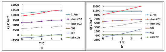
Figure 2.
The model outputs for the “steady”—(a), and “unsteady”—(b) scenarios of air temperature changes by +1 °C, +2 °C, +3 °C, and +4 °C.
An evenly distributed increase in the average annual temperature (T) had a minor effect on the annual flux G_Psn, but it was found to be a driver of other annual fluxes: CO2, NEE, CH4, NO, and N2O. Following a seasonally biased scenario of temperature increase (Ta), with a temperature set-up variable over months, an increase in all annual fluxes was revealed.
The comparison of data from two simulated scenarios with the data of the base model in terms of relative deviation (RD) is presented in Table 3.
Table 3.
Relative deviation (RD) of cumulative annual modeled air temperature rises and corresponding carbon (C) and nitrogen (N) fluxes, in %; where Tk °C is annual increase in air temperature (Ta) by k °C, and the other variables are similar to these presented in Table 2.
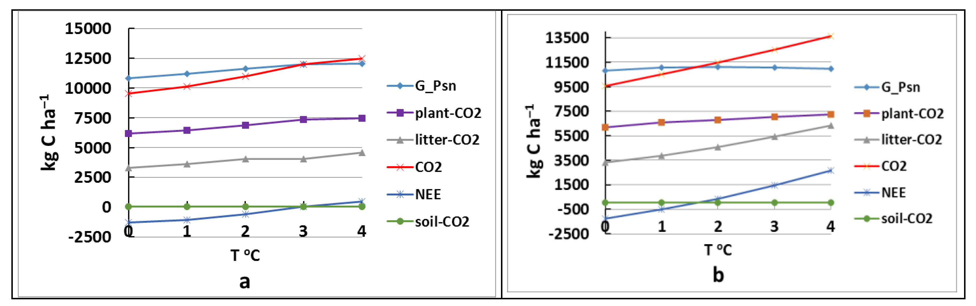
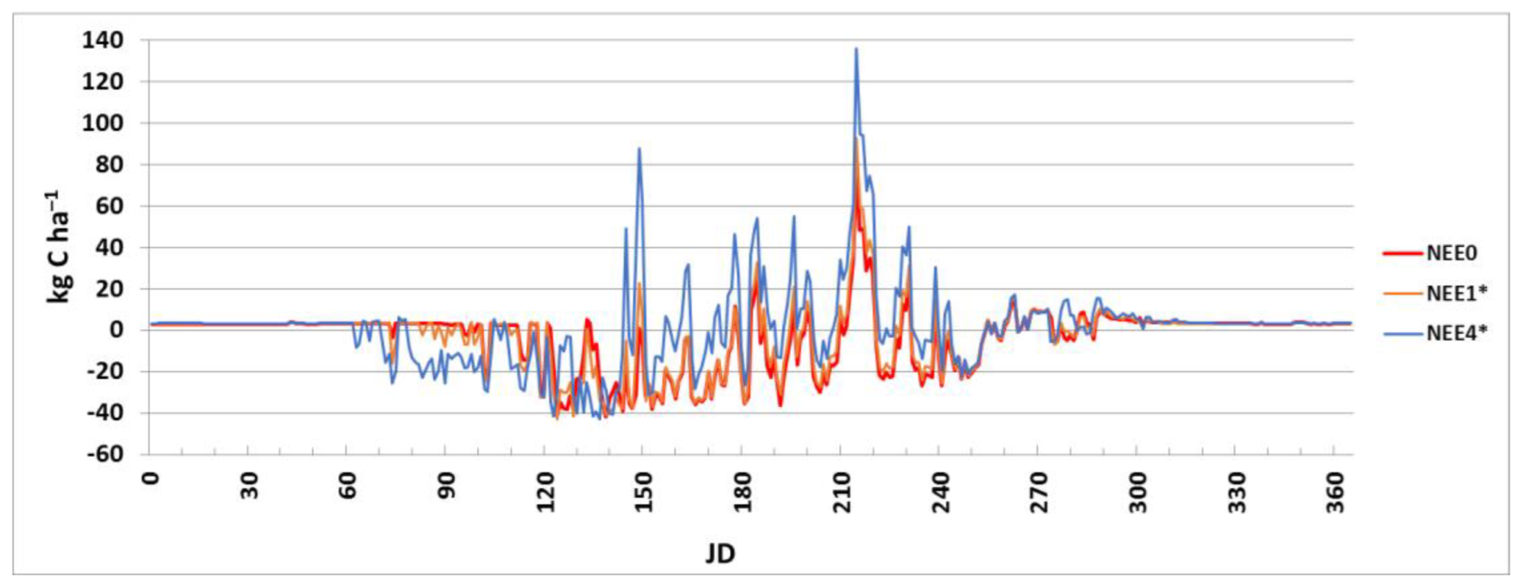
Scenario 1 of air temperature changes (see Table 2 for details) was studied at the test site of Great Vasyugan Mire with the reference year of 2019 and the base model, k = 0 °C. The changes were an increase in T* of 1 °C (Tk1 compared to the base model in Table 2) followed by an increase in annual NEE by a relative deviation (RD) of 58.6%, an annual CH4 by RD of 22.9%, and an annual G_Psn by RD of 2.2%. At the next step, the temperature rise of 2 °C (Tk2 compared to the base model in Table 2) leads to an increase in annual NEE by RD of 128.5%, an annual CH4 by RD of 50.0%, and an annual G_Psn by RD of 2.6%. A further increase in temperature leads to an increase in all annual GHG fluxes except for G_Psn. Along with the growth in the annual NEE (Table 2), the growth in the average daily NEE is also illustrated in Figure 3. Thus, under scenario 1 of air temperature increase, we observe somewhat different strengths impact on the annual GHG fluxes: an insignificant non-monotonic effect on G_Psn, a weak monotonic effect on the annual plant-CO2 flux, and a strong monotonic effect on the annual fluxes of CO2 and CH4, as well as NO, N2O, and NEE.
Figure 3.
The model output of net ecosystem exchange (NEE, kg C ha−1) constrained by daily air temperature (Ta): for 0 °C (NEE0), for +1 °C (NEE1*) and +4 °C (NEE4*) temperature increase); JD—Julian day.
In scenario 2 of air temperature increase, changes (T*) by k °C (details presented in Table 2) were studied at the same test site with a reference year of 2019. The months of February, March, May, and October were found to be the main drivers of annual temperature increase. The temperature increase in 1 °C (Tk1* compared to the base model) led to an increase in annual NEE by a relative deviation (RD) of 17.0%, an annual CH4 by RD of 22.0%, and an annual G_Psn by RD of 3,3%. The temperature increase in Ta of 2 °C (corresponding to T2* as compared to T0 in Table 2) led to an increase in annual NEE by an RD of 53.2%, an annual CH4 by RD of 50.0%, and an annual G_Psn by RD of 7.3%. A further increase in Ta led to an increase in all annual GHG fluxes.
The simulated values of C and N fluxes in scenario 1 of air temperature change differ from the same values simulated under scenario 2 of air temperature change. We suspect that scenario 2 should be considered as a typical climatic scenario at the study site (and basically at other boreal peatland sites) to ensure better accuracy of modeling studies.
According to Table 2, when comparing the even (Tk) and uneven/variable temperature increments (Tk*) related to the monthly Ta, one can reveal a clear acceleration in the growth of G_Psn* relative to G_Psn, the same way as CH4 accelerate the growth relative to CH4*; but the slowdown revealed in the growth of CO2*, NEE*, NO*, and N2O* is relative to CO2, NEE, NO, and N2O, respectively.
The modeled scenarios of interactions between air temperature increase and the carbon balance (namely, NEE) let us make certain conclusions on whether the ecosystems represent the sink (annual average NEE < 0) or the source (annual average NEE > 0) of atmospheric carbon, and to determine the point of the switch from one state to the other. We found that the NEE is going to reach this “zero” point with Ta +1.6 °C simulated with scenario 1 of temperature increase (Tk), whereas it is going to happen with Ta +3.0 °C when simulated with scenario 2 of temperature increase (Tk*).
Basically, the temperature growth is in good correlation with the growth of annual NEE (NEE = CO2 − G_Psn), and it is supported by the growth of CO2 flux but almost stable values of G_Psn (see Table 2; Figure 2).
At the same time, the variable of plant-CO2 makes a greater contribution to the growth of CO2 flux: it varies from 65% for T0 to 53% for T4 (Table 2; Figure 2). In the case of Tk*, the NEE* flux slowed down its growth rate compared to the NEE for Tk due to a gradual (or monotonic) slowdown in the growth of litter-CO2* relative to litter-CO2 and an acceleration of the growth of G_Psn* relative to G_Psn, as shown in Figure 2. It is supported by a slight increase in plant-CO2*, relative to plant-CO2, and a decrease in the contribution of plant-CO2* to CO2* to 60% for Tk4* (Figure 2).
The determination coefficient (R2) was used to estimate the accuracy of our modeling study. In the case of linear regression (based on the method of least squares and analysis of variance), R2 is equal to the square of the Pearson correlation coefficient (r) between the values of different variables (Table A2 in Appendix A, Figure 2). In our case of evenly distributed temperature increase, R2 decreases (with differences between variables tend to increase) from 0.94 (between NEE1* and NEE0) to 0.39 (between NEE4* and NEE0). At the same time, the differences between simulations under scenarios 1 and 2 also increase; R2 decreases from 0.97 (between NEE1* and NEE1) to 0.81 (between NEE4* and NEE4).
To assess the heterogeneity of the simulated daily variants of interactions between air temperature and NEE, we estimated the values of NEE in addition to implementing a non-parametric analysis of variance in order to compare the values of NEE (see Figure A3 in Appendix A). The air temperature vs. NEE parameters were studied with the Kruskal–Wallis test. It was found to be insignificant (p > 0.1) (differences between NEE1* and NEE0 or NEE1* and NEE1), with a +1 °C temperature increase, whereas it was found strongly significant (0.001 < p < 0.01) with a +4 °C temperature increase (differences between NEE4* and NEE0 or NEE4* and NEE4).
3.2. Simulation Modeling of Precipitation
Simulation modeling of changes in precipitation (P) was implemented with two different scenarios: the maximum and the minimum annual precipitation. The years 2012, 2018, and 2019 with weather conditions prescribed in these precipitation scenarios were found in the long-term climatic data set (http://meteo.ru/) (URL accessed on 1 December 2022). We used the data on the intra-annual (monthly) distribution of precipitation for the period of 1970–2020. Amongst the years, the average long-term precipitation (431 mm) corresponds to 2019. The minimum precipitation (321 mm) was found in 2012, and the maximum precipitation of 677 mm corresponded to 2018. In order to simulate extreme climate changes in the annual rate of precipitation, a decrease of 2.5 times and an increase of 3 times have been studied. The decrease in annual precipitation (P) was set up compared with the baseline value of 430 mm at the rate of annual precipitation—380 mm, 320 mm, 240 mm, and 160 mm. In terms of geo-climatic conditions, the precipitation of 380 mm corresponds well to the dry steppe climatic region, and the precipitation of 160 mm corresponds to the subboreal desert region. An increase in the annual mean precipitation (P*) was set up at the rates of 550 mm, 680 mm, 1020 mm, and 1350 mm, with the last step corresponding to precipitation values in the subtropics. An increase in annual precipitation was studied with the base year of 2019.
The study has found no evidence of significant change in the annual NEE simulated under the increased precipitation scenario at any of the analyzed precipitation rates (presented in Table 4 and in Figure 4).
Table 4.
The model outputs of annual precipitation (P, mm) and the fluxes of carbon—C (kg C ha−1) and nitrogen—N (g N ha−1).
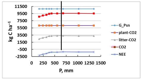
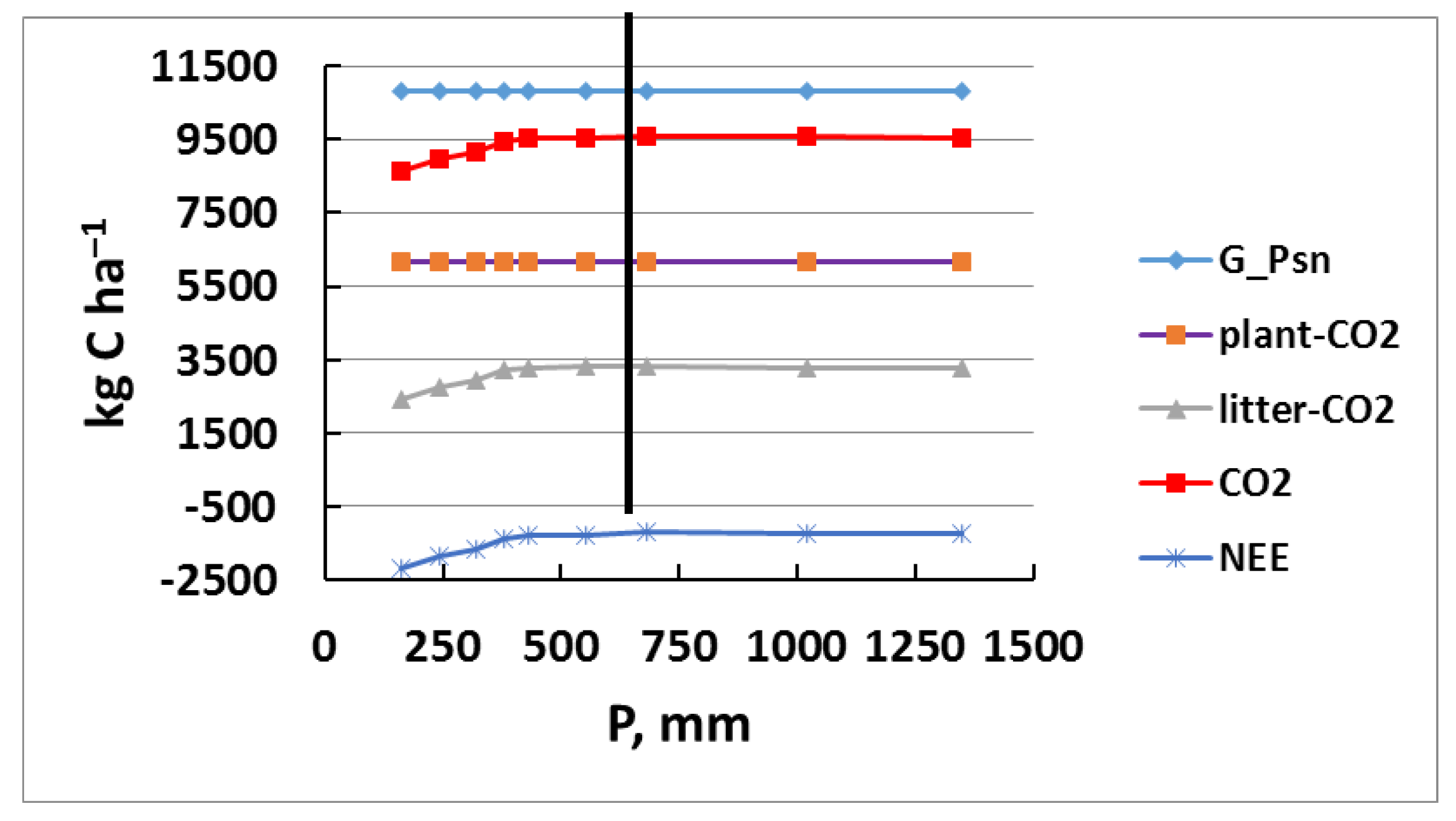
Figure 4.
The model outputs of carbon fluxes simulated under different precipitation scenarios (P, mm). G_Psn—total gross photosynthesis; plant-CO2—plant respiration; litter-CO2—carbon dioxide after mineralization of litter; CO2—total flux of carbon dioxide; NEE—Net Ecosystem Exchange. The baseline model results are marked with a vertical line.
A decrease in annual precipitation in the range from 430 mm to 160 mm led to a gradual decrease in the annual net ecosystem exchange (NEE) due to a change in the annual CO2 flux with the same total gross photosynthesis (G_Psn).
The comparison of the simulated scenarios of precipitation with the initial base model results in terms of relative deviation (RD) is presented in Table 5.
Table 5.
Relative deviation (RD) of simulated cumulative annual precipitation patterns and changes in carbon (C) and nitrogen (N) fluxes, in %.
Here, we reveal that the relative deviation of the annual NEE is limited to RD ≤ 5.2% in the case of a humid climate, and the module of relative deviation of the annual NEE |RD| ≤ 71.3% in the case of a dry climate. The annual CH4 flux decreases gradually under both an increase and a decrease in annual precipitation scenarios (|RD| ≤ 5.1%). One can consider the current climatic conditions in terms of precipitation as the climatic optimum of methane (CH4) emissions. The annual fluxes of NO and N2O increase significantly (by 9.4 and by 3.3 times, for NO and N2O, respectively) with an increase in annual precipitation. The model outputs of daily variants of precipitation vs. NEEk are presented in Figure 5.
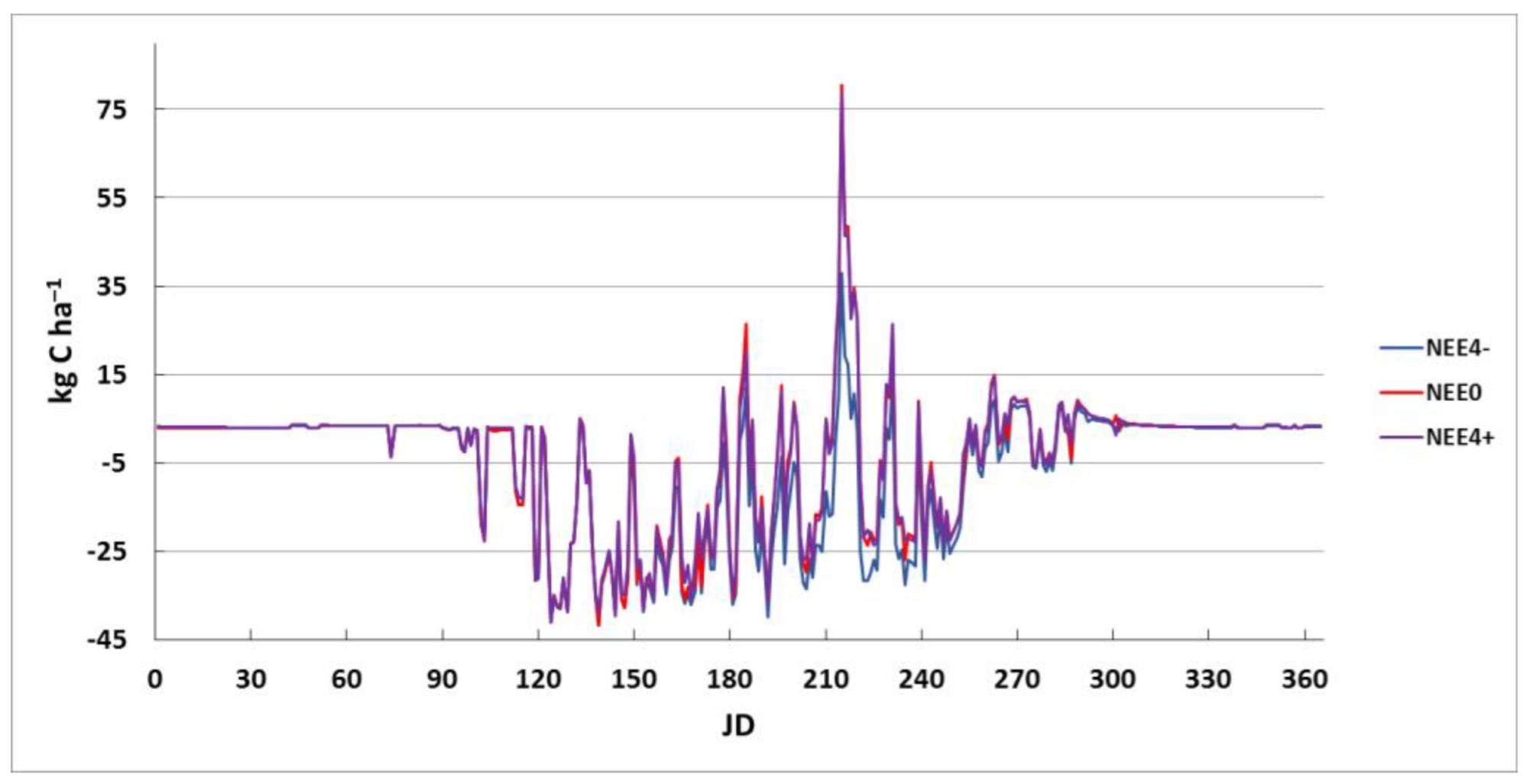
Figure 5.
The model outputs of daily variants of precipitation (P) and net carbon exchange: NEE4− (annual precipitation P = 160 mm), NEE0 (annual precipitation P = 430 mm), and NEE4+ (annual precipitation P = 1350 mm).
The accuracy of simulation modeling for the scenarios of annual NEEk under conditions of precipitation change was assessed by correlation coefficients (R2) (Table A3, Appendix A). The highest correlation coefficients were found between NEEk+, and the smallest correlation coefficients were found between NEE4− and NEEk+. A scatterplot with a direct linear regression for dry and humid climates, confirming the accuracy of simulation modeling, is shown in Figure A4, Appendix A. It also shows the differences between the models of dry and humid climates tend to increase; R2 decreases from 0.99 (between NEE4+ and NEE0) to 0.89 (between NEE4− and NEE0).
The precipitation change vs. NEE was studied with the Kruskal–Wallis test. Its relation was found insignificant (p > 0.1) in humid climates (differences between NEE4+ and NEE0), whereas it was found highly significant (0.001 < p < 0.01) in dry climates (differences between NEE4− and NEE0) (see Figure A5, Appendix A; Table A4, Appendix A).
3.3. Simulation Modeling of Groundwater (Water Table)—WT
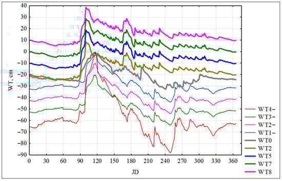
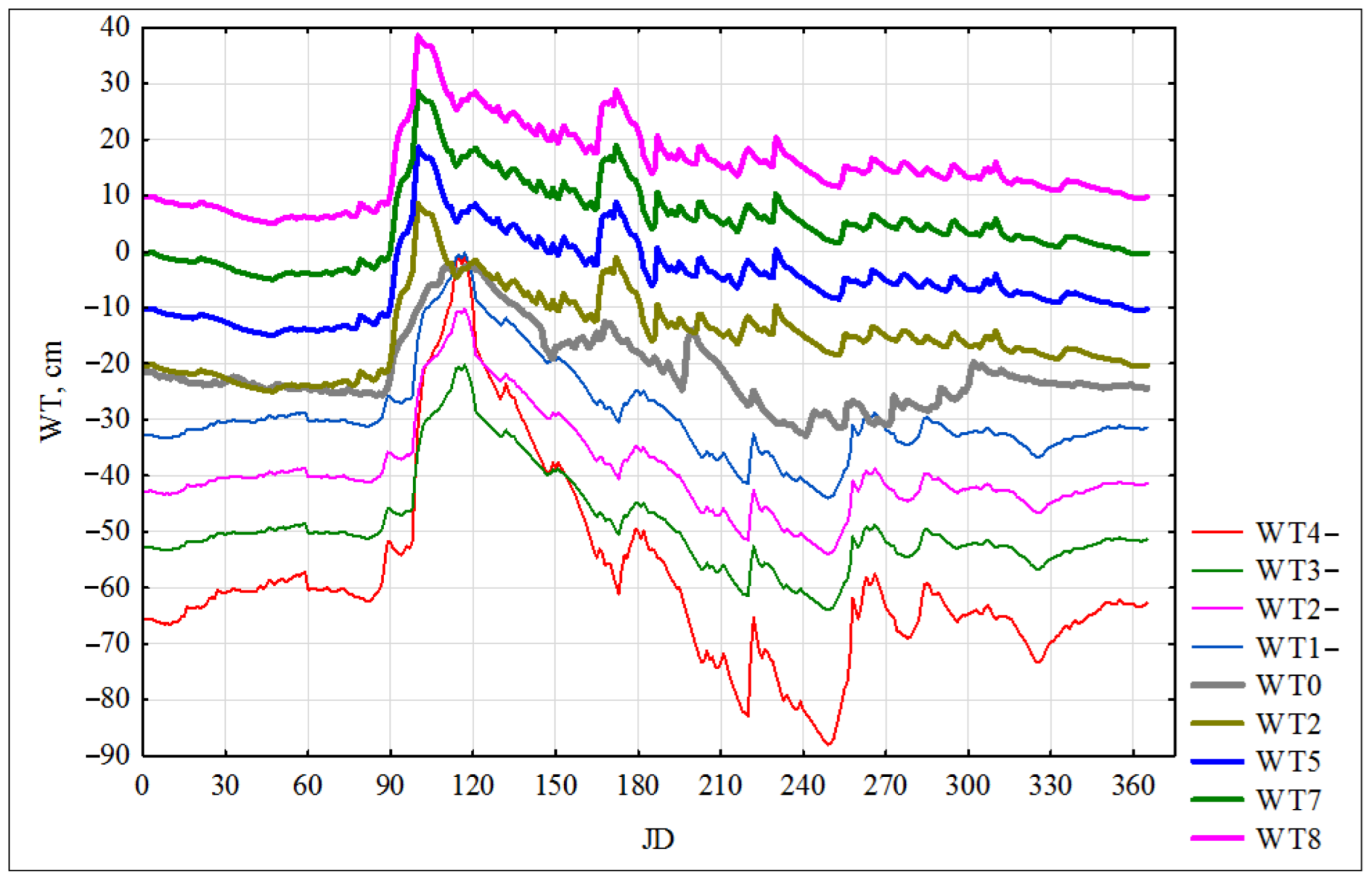
Simulation modeling of GHG fluxes, in terms of changes in groundwater level with the Wetland-DNDC model, was carried out in a similar way to previous studies with “decrease” and “increase” scenarios of average annual groundwater levels (WTk) at a wetland site in Ontario, Canada [20]. The decrease scenario was set up with −102 cm (WT5-), −58 cm (WT4-), −49 cm (WT3-), −39 cm (WT2-), and −29 cm (WT1-) groundwater levels. The increase scenario was set up with −18 cm (WT1), −15 cm (WT2), −12 cm (WT3), −8 cm (WT4), −5 cm (WT5), −1 cm (WT6), 5 cm (WT7), and 15 cm (WT8) groundwater levels. The distribution of groundwater levels by month corresponds to the average levels, which have been measured directly at our study site in the period of 2013–2019. Our simulations were also made in extreme conditions in order to evaluate ecosystem exchange with the average annual critical mark of +15 cm representing the conditions of flooding, as well as −102 cm representing the minimum water table or extreme dry conditions that could be observed at wetland sites [44]. With respect to these conditions, the daily variations of the WT were modeled in Wetland-DNDC for the range of WT from −58 cm to 15 cm. The results are presented in Figure 6.
Figure 6.
The model outputs of the (daily) groundwater level (WTk) in the range of annual mean water table of −58 cm to 15 cm; for the WT0 (WT = −21 cm) at the model study site of Great Vasyugan Mire (GVM) in 2019.
The model results are shown in Table 6. With an increase in the average annual WT in the range of −102 cm to 15 cm, we have found the GHG fluxes changed gradually but with different rates; namely, the gross photosynthesis (G_Psn) had almost no change (decreased by 1.04 times only), whereas the CO2 decreased at some moderate rate (by 2.4 times). The groundwater level has a significant impact on the modeled NEEs: the NEE values decrease from 4800 to –3700 kg C ha−1 within prescribed groundwater levels. The decrease in the annual NEE (NEE = CO2 − G_Psn) with an increase in the groundwater level occurs due to a decrease in CO2 fluxes with almost stable gross photosynthesis (G_Psn). At the same time, the litter-CO2 and soil-CO2 make a greater contribution to the decrease in CO2 flux with a slight change in plant-CO2. Notably, the N2O decreases with great rate (192.6 times) and NO decreases by 1500 times. At the same time, the CH4 flux increases with an increase in the groundwater level from 0 to 2900 g C ha−1. Also, we note that when starting the WT ≥ −1 cm, all flux curves reach the plateaus.
Table 6.
The model outputs of the annual mean fluxes of carbon (kg C ha−1) and nitrogen (g N ha−1) at different groundwater levels (WT, cm).
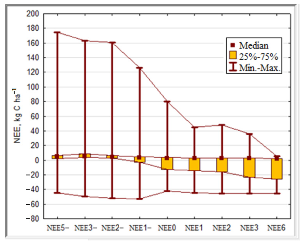
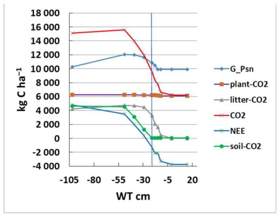
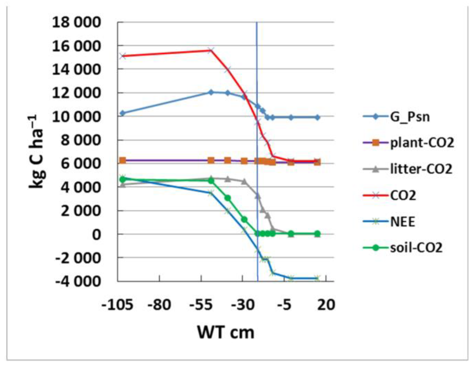
The data in Table 6 revealed that starting from WT level ≥ −28 cm, the annual NEE flux turned to be a negative value, which meant that the ecosystem began to act as a carbon sink rather than a source (NEE < 0 in Figure 7). At the same time, separate intervals of negative average daily fluxes NEE < 0 were also observed at WT < −28 cm (Figure 8).
Figure 7.
The model outputs of carbon fluxes (kg C ha−1) for different scenarios of change in groundwater level (WT, cm). The baseline model results are marked with a vertical line.
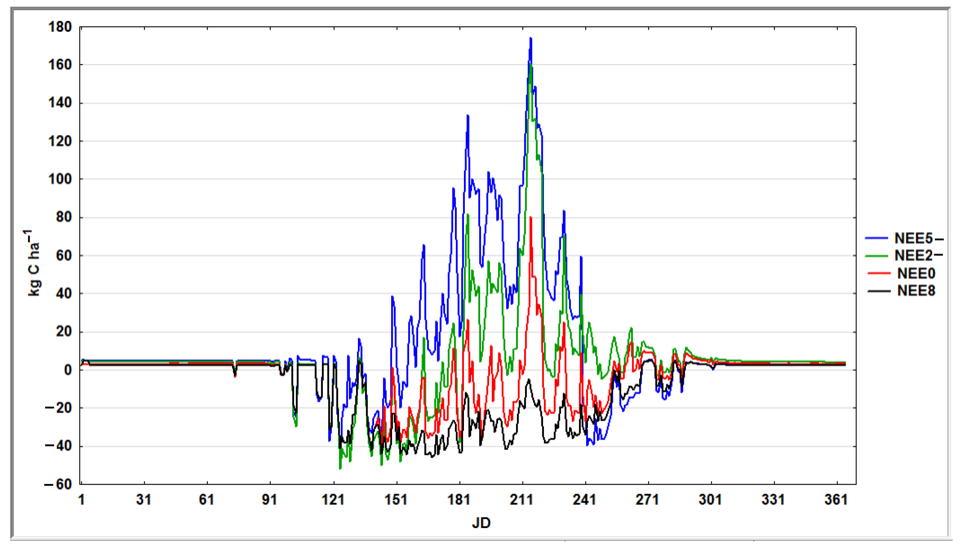
Figure 8.
The model outputs of daily variants of groundwater level (WTk): the annual mean water table range −102 cm to 15 cm and net ecosystem exchange (NEE, kg C ha−1).
An accuracy assessment of the simulated scenario data of groundwater level measurements, with the initial data of the base model in terms of relative deviation (RD), is given in Table 7.
Table 7.
Relative Deviation (RD) of simulated cumulative annual groundwater levels and corresponding carbon (C) and nitrogen (N) fluxes, in %.
The study revealed that in the conditions of WT decrease to the model −102 cm in reference to the baseline level of 2019 (−21 cm) by the relative deviation RD of −386%, the annual NEE flux increases to the model by 4801 kg C ha−1 compared to the initial −1283 kg C ha−1 by a relative deviation RD of 474%. Also, with an increase in WT to the model 15 cm in reference to the initial −21 cm by a relative deviation RD = 171%, the annual NEE flux decreased in the model by −3746 kg C ha−1 compared to the initial −1283 kg C ha−1 (relative deviation RD of −192%).
Correlation coefficients between NEE and groundwater levels are listed in Table A5, Appendix A. For instance, WT decreased from the original −21 cm (NEE0) to the model −102 cm (NEE5−), leading to an increase in the differences between NEE0 and the corresponding model NEEk: R2 decreases from 0.68 between NEE1− and NEE0 to 0.11 between NEE5− and NEE0 (Figure A6, Appendix A).
The test of Kruskal–Wallis revealed that change in precipitation highly significantly affects NEE (p < 0.001) as WT decreases from −21 cm to −102 cm (difference between NEEk− and NEE0), and it is very significant (0.001 < p < 0.01) with an WT increase from −21 cm to 15 cm (differences between NEEk+ and NEE0) (Figure A7, Appendix A; Table A6, Appendix A).
4. Discussion
The net ecosystem exchange (NEE) is a measure of ecosystem function that acts either as a sink or as a source of atmospheric carbon. In the Wetland-DNDC model, this process is represented by two basic equations: (i) accumulation of carbon via photosynthesis (G_Psn) and (ii) emissions/fluxes of carbon dioxide (CO2). Overall, this study revealed a high correlation between the temperature (T), precipitation (P), and groundwater/water table (WT) variables and both the fluxes of greenhouse gases (GHG) and Net Ecosystem Exchange (NEE). Especially, the growth in air temperature seems to affect the growth of the annual NEE, supported by the growth of CO2 fluxes. The heterogeneity of the distribution of precipitation by months within a year is important.
In detail, the evenly distributed increase in the average annual temperature (T) had no effect or led to a very minor increase in the total gross photosynthesis (G_Psn), but it affected more significantly the fluxes of greenhouse gases: CO2, NEE, CH4, NO, N2O. Under scenario 2 (or monthly-different) increase in the average annual temperature, an increase in all annual fluxes has been observed. The NEE* slowed down the growth rate compared to NEE due to a gradual slowdown in the growth of litter-CO2* compared to litter-CO2 and an acceleration of the growth of G_Psn* compared to G_Psn. Also, there was a slight increase in plant-CO2* relative to plant-CO2, and a decrease in the contribution of plant-CO2* to CO2* has been observed. Under scenario 1 increase in T, the growth of the annual NEE (NEE = CO2 − G_Psn) is supported by the growth of CO2 flux with almost stable values of gross photosynthesis (G_Psn). At the same time, plant-CO2 makes a greater contribution to the growth of CO2 flux. In line with model studies in Canadian peatlands [45], our study demonstrates a rather minor effect of high-temperature rise to CO2 flux and sinks than that of moderate rise of air temperatures.
Similar conclusions on the effect of temperature on NEE and CH4 fluxes are presented by Zhang et al. [13]. In addition, the other model results indicate that possible warming can potentially lead to a certain increase in CO2 fluxes from peat bogs into the atmosphere, considering peat bogs in Western Siberia and a wide range of wetlands in other geographical locations [9,46].
An increase in annual precipitation in the range of 430–1350 mm does not lead to a significant change in the annual NEE (Table 4). A decrease in annual precipitation in the range of 430–160 mm leads to a gradual decrease in the annual NEE due to a change in the annual CO2 flux with the same G_Psn. As a result, the growth of annual precipitation in the range of 160–1350 mm leads to an increase in annual NEE by 1.81 times (from −2198 to −1216 kg C ha−1). This transformation, however, is not enough to change our ecosystem (mire site) from carbon sink (annual NEE < 0) to carbon source (annual NEE > 0). The annual CH4 flux decreases both with an increase and a decrease in annual precipitation, which means one should consider the current climatic conditions in terms of precipitation as a sort of climatic optimum for methane emission. Finally, with an increase in annual precipitation, the annual fluxes of NO and N2O increase accordingly.
The change in groundwater level significantly affects the Net Ecosystem Exchange (NEE). Namely, the greenhouse gas fluxes increase as follows: N2O by 230 times and NO by 1900 times. The CH4 flux increases as the groundwater level increases from 0 to 2891 g C/ha.
With an increase in the average annual WT from −102 cm to 15 cm, GHG fluxes change at different rates: G_Psn decreases slightly, CO2 decreases at a moderate rate, and NEE decreases significantly (from 4800 to −3700 kg C ha−1) due to a decrease in litter-CO2 and soil-CO2 supported by a minor change in plant-CO2. In the conditions of rising water levels corresponding to WT ≥ −28 cm, the model runs revealed the negative annual NEE fluxes, which meant that the mire ecosystem turned out to be a carbon sink (NEE < 0). At the same time, a few intervals of negative average daily fluxes of NEE < 0 were also observed at WT < −28 cm. Our studies of groundwater levels vs. GHG fluxes are very consistent with some previous studies [19,47], which showed that a decrease in groundwater levels leads to CH4 emissions reduction and a rise om CO2 emissions from soils. It also confirms the study by Webster et al. [20], who have found that drought leads to an increase in CO2 fluxes and a decrease in CH4 flux.
At present, different scientific publications stand on different points of view on the current carbon status of terrestrial ecosystems, i.e., whether they tend to be a carbon sink or a carbon source. There are a few studies that agree with the idea of full and persistent stock of atmospheric carbon in terrestrial ecosystems of Northern Eurasia [15,28]. At the same time, there are some studies that tend to doubt this idea [48]. Also, there are a number of studies that consider wetland ecosystems, both the sink and the source of atmospheric carbon, as ecosystems with rather immediate reactions to ongoing climate change [49,50,51]. The data from the middle boreal region of Western Siberia (Mukhrino test site) revealed the net CO2 fluxes varied in a wide range from negative (–32.1 g C m–2 in 2019) to positive (13.4 g C m–2 in 2017) values [31,52]. Certain evidence of change in carbon status, from source (annual NEE > 0) to sink (annual NEE < 0), was found in European Russia peat bogs [15]. According to studies by Golovatskaya et al. [53], the Pine-dwarf shrub-Sphagnum bog ecosystems in the south taiga region of Western Siberia represent the sink of atmospheric carbon during the whole time period of 1999−2007.
The Wetland-DNDC model in our study took into account the change in main hydrothermal environmental conditions (namely, Ta, P, and WT) and investigated the way it affects greenhouse gas fluxes; also, the model simulated conditions of an annual NEE < 0, same way as in Golovatskaya et al. [53].
In the case of an evenly distributed increase in air temperature (Ta), NEE is going to reach a “zero” point with a Ta increase of 1.6 °C, and in the case of a seasonally biased increase in air temperature, it is going to happen at 3.0 °C. Our model simulations of groundwater table (WT) vs. NEE also allow for a change from sink to source when the WT drops by ≈7 cm (from −21 cm to −28 cm with reference to the level of the ground). With an increase in the annual precipitation in the range of 16- to 135 mm, the model suggests a weak increase in an annual NEE by 1.81 times (from −2198 to −1216, kg C ha−1), which is not enough to change ecosystem functions from sink (annual NEE < 0) to source (annual NEE > 0). The length of the growing season is the most important factor in constraining NEE [42].
5. Conclusions
The study confirmed the good ability (R2 = 0,675) of the Wetland-DNDC biogeochemical model to perform ecosystem modeling at the test site of the Great Vasyugan Mire (GVM), the largest wetland massif in the world. The model estimated the fluxes of greenhouse gases (GHG) for a few scenarios of change in environmental (hydrothermal) conditions, namely (i) air temperature, (ii) precipitation, and (iii) groundwater table. The evenly distributed increase in the average annual temperature (T) led to a minor increase in the total gross photosynthesis (G_Psn), but it affected more significantly the fluxes of greenhouse gases: CO2, NEE, CH4, NO, and N2O. Under a scenario of a seasonally biased (or monthly-different) increase in the average annual temperature, an increase in all annual fluxes has been observed. The study of different scenarios of change in annual air temperature revealed the threshold of change in the wetland/peatland ecosystem from carbon sink to carbon source to the atmosphere, which is going to happen with an increase in the average annual air temperature by 3 °C compared with current values. A change in annual precipitation in the range from 430 mm to 1350 mm did not lead to a significant change in the annual NEE, then did not lead to reverse the sink-to-source categories of carbon storage. Changes in groundwater levels were found to be the most powerful driver of annual NEE fluxes, especially as they increase. The wetland/peatland ecosystem turn to act as an active carbon sink with about a 7 cm increase in the annual groundwater level, compared with its base level of 21 cm.
Author Contributions
Conceptualization. A.M., I.G. and S.V.; methodology. A.M. and Y.K.; software. A.M. and E.B.; validation. Y.K., A.M., E.A. and E.B.; formal analysis. A.M., V.N. and S.V.; investigation. Y.K. and E.B.; data curation E.A. and Y.K.; writing—original draft preparation. A.M., Y.K. and S.V.; writing-review and editing. S.K. and E.N.; visualization. A.K. and E.N. All authors have read and agreed to the published version of the manuscript.
Funding
This study was supported by the Tomsk State University Development Programme («Priority-2030») and the Ministry of Education and Science of Russia No. 0533-2021-0004 and № FSWM-2023-0005. RFBR grant 20-34-90090. The study was carried out by using the equipment of the Unique Research Installation “System of experimental bases located along the latitudinal gradient” TSU with financial support from the Ministry of Education and Science of Russia (RF-2296.61321X0043, 13УHУ. 21.0005, agreement No. 075-15-2021-672). RSF grant 23-14-20015 “Study of patterns of carbon stock formation in biological systems and landscapes in the transition space from North Asia to Central Asia” for Tuva State University.
Conflicts of Interest
The authors declare no conflict of interest.
Appendix A
Table A1.
Model input parameters [User’s Guide for Wetland-DNDC] and its values at Bakchar test site (Great Vasyugan Mire, Western Siberia) in 2019.
Figure A1.
Daily average air temperature (Tav, °C), precipitation (P, mm), and groundwater table (WT) in 2019.
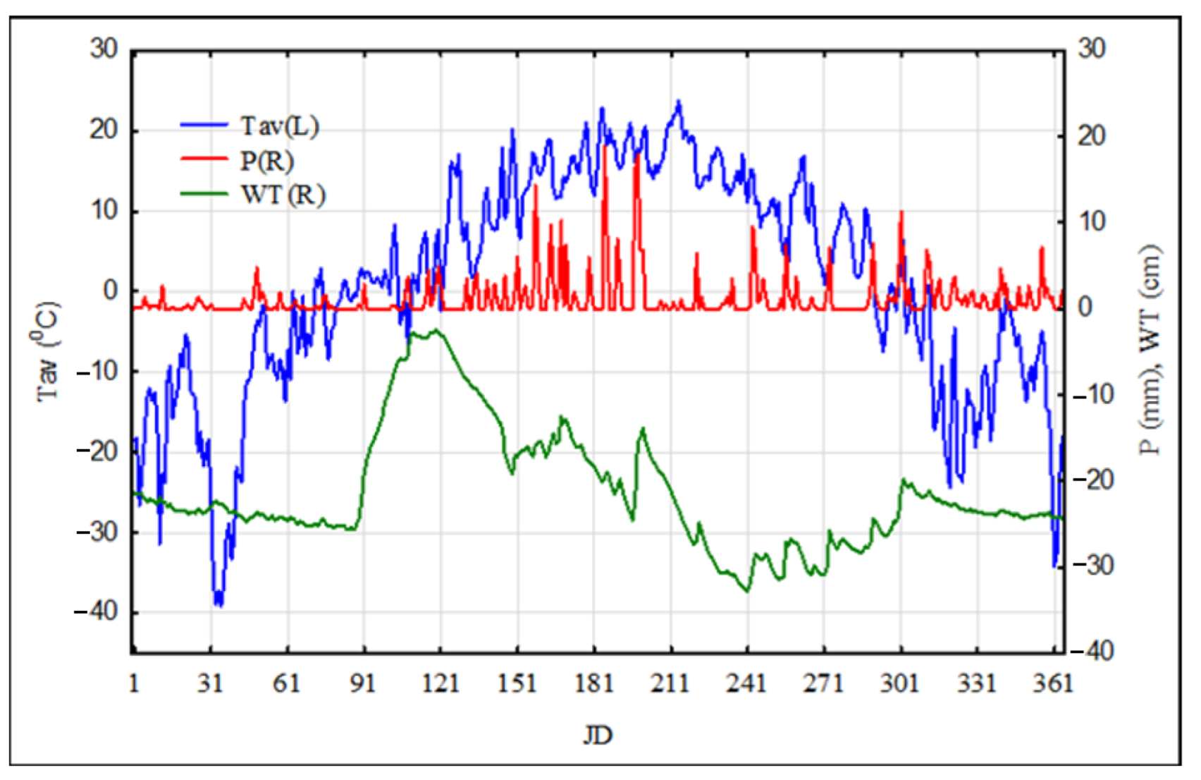
Table A2.
Correlation coefficients: non-parametric (NEEx), Spearman (Rs), and parametric Pearson (r) after model runs with air temperature changes.
Figure A2.
Direct linear regression for 1 degree of warming NEE0 and NEE1* (a) and 4 degrees of warming NEE0 and NEE4* (b).
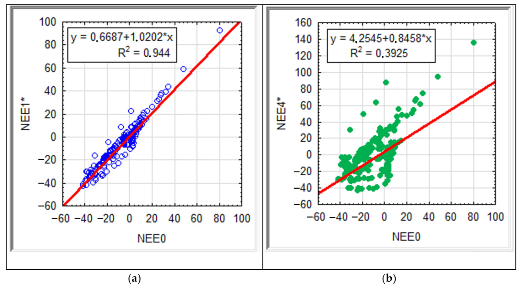
Figure A3.
The options of air temperature change vs. net ecosystem exchange (NEEx).
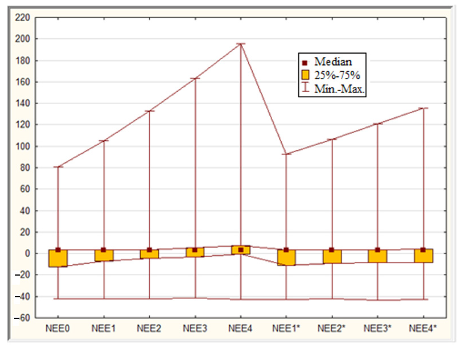
Table A3.
Correlation coefficients: non-parametric (NEEx), Spearman (Rs), and parametric Pearson (r) after model runs with precipitation changes.
Figure A4.
Direct linear regression for (a) dry climate (reduction in annual precipitation from 43 mm to 16 mm) NEE0 and NEE4−, and (b) humid climate (increase in annual precipitation from 43 mm to 135 mm) NEE0 and NEE4+.
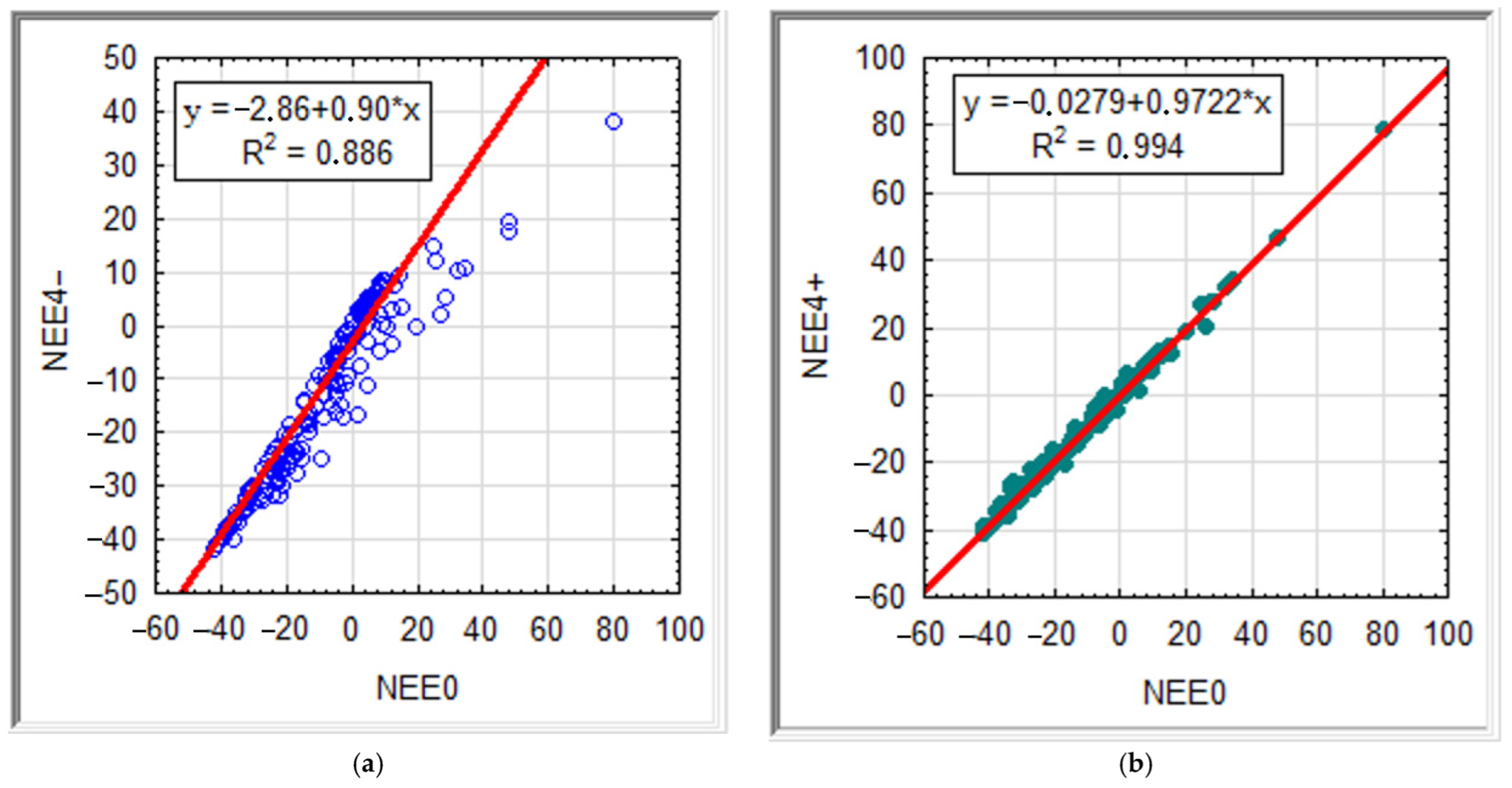
Figure A5.
The options of precipitation (P) change (increase in annual precipitation from 16 mm to 135 mm) vs. net ecosystem exchange (NEEx).
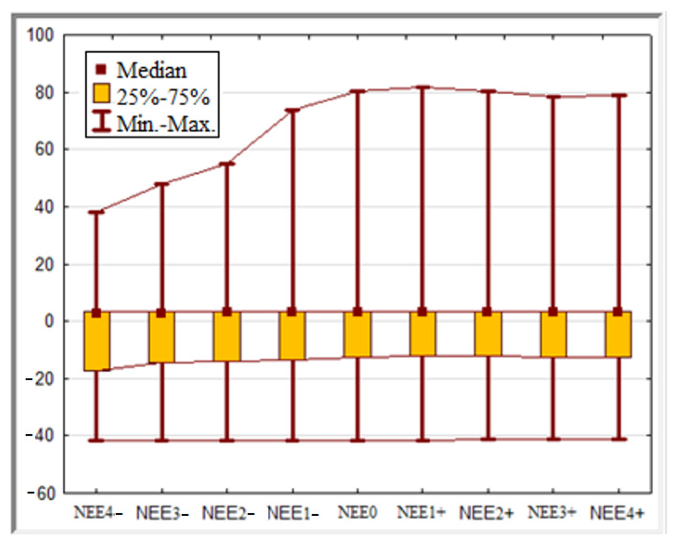
Table A4.
Numerical parameters of NEEx vs. precipitation (P).
Table A5.
Correlation coefficients: non-parametric (NEEx), Spearman (Rs), and parametric Pearson (r) after model runs with changes in water table (WT). The bold letters correspond to significant correlation coefficients.
Figure A6.
Direct linear regression for NEE0 and NEE5− (a) and for NEE0 and NEE1− (b).
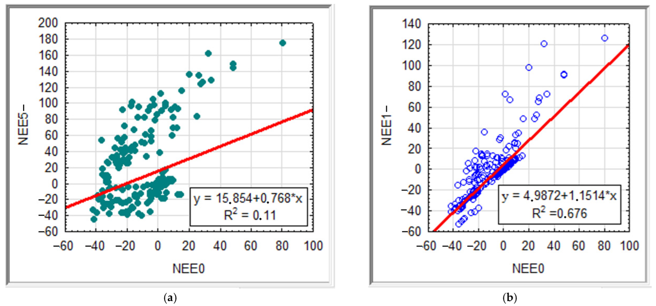
Table A6.
Numerical parameters of NEEx vs. groundwater table (WTk).
Figure A7.
The options of groundwater table (WTk) change (from −102 cm to −1 cm of annual mean WT) vs. net ecosystem exchange (NEEx).
References
- Eswaran, H.; Van den Berg, E.; Reich, P.; Kimble, J. Global soil carbon resources. In Soils and Global Change; Lal, R., Ed.; CRC Press: Boca Raton, FL, USA, 1995; pp. 27–43. [Google Scholar]
- Bubier, J.L.; Crill, P.M.; Moore, T.R.; Savage, K.; Varner, R.K. Seasonal patterns of controls on net ecosystem CO2 exchange in a boreal peatland complex. Global Biogeochem. Cycles 1998, 12, 703–714. [Google Scholar] [CrossRef]
- Silvola, J.J.; Alm, U.A.; Ahlholm, U.; Nykanen, H.; Martikainen, P.J. CO2 fluxes from peat in boreal mires under varying temperature and moisture conditions. J. Ecol. 1996, 84, 219–228. [Google Scholar] [CrossRef]
- Shurpali, N.J.; Verma, S.B.; Kim, J.; Arkebauer, T.J. Carbon dioxide exchange in a peatland ecosystem. J. Geophys. Res. 1995, 100, 14319–14326. [Google Scholar] [CrossRef]
- Li, C. Quantifying greenhouse gas emissions from soils: Scientific basis and modeling approach. Soil Sci. Plant Nutr. 2007, 53, 344–352. [Google Scholar] [CrossRef]
- Giltrap, D.L.; Li, C.; Saggar, S. DNDC: A process-based model of greenhouse gas fluxes from agricultural soils. Agric. Ecosyst. Environ. 2010, 136, 292–300. [Google Scholar] [CrossRef]
- Gilhespy, S.L.; Anthony, S.; Cardenas, L.; Chadwick, D.; del Prado, A.; Li, C.; Misselbrook, T.; Rees, R.M.; Salas, W.; Sanz-Cobena, A.; et al. First 20 years of DNDC (DeNitrificationDeComposition): Model evolution. Ecol. Model. 2014, 292, 51–62. [Google Scholar] [CrossRef]
- Janse, J.H.; Van Dam, A.A.; Hes, E.M.; de Klein, J.J.; Finlayson, C.M.; Janssen, A.B.; van Wijk, D.; Mooij, W.M.; Verhoeven, J.T. Towards a global model for wetlands ecosystem services. Curr. Opin. Environ. Sustain. 2019, 36, 11–19. [Google Scholar] [CrossRef]
- Song, C.; Luo, F.; Zhang, L.; Yi, L.; Wang, C.; Yang, Y.; Li, J.; Chen, K.; Wang, W.; Li, Y.; et al. Nongrowing Season CO2 Emissions Determine the Distinct Carbon Budgets of Two Alpine Wetlands on the Northeastern Qinghai—Tibet. Atmosphere 2021, 12, 1695. [Google Scholar] [CrossRef]
- Sukhoveeva, O.E. Modeling of greenhouse gas fluxes and nitrogen and carbon cycles in soils (review). J. Nat. Sci. Res. 2017, 2, 61–76. (In Russian) [Google Scholar]
- Mitsch, W.J.; Sraskraba, M.; Jorgensen, S.E. (Eds.) Development in Environmental Modeling. In Wetland Modeling; Elsevier Science: New York, NY, USA, 1988; Volume 12, p. 227. [Google Scholar]
- Cui, J.B.; Li, C.S.; Trettin, C. Analyzing the ecosystem carbon and hydrologic characteristics of forested wetland using a biogeochemical process model. Glob. Change Biol. 2005, 11, 278–289. [Google Scholar] [CrossRef]
- Zhang, Y.; Li, C.; Trettin, C.C.; Li, H.; Sun, G. An integrated model of soil, hydrology, and vegetation for carbon dynamics in wetland ecosystems. Glob. Biogeochem. Cycles 2002, 16, 1061. [Google Scholar] [CrossRef]
- User’s Guide for Wetland-DNDC, USA. Available online: https://www.dndc.sr.unh.edu/model/ForestUserGuide.pdf (accessed on 1 April 2023).
- Kurbatova, J.; Li, C.; Tatarinov, F.; Varlagin, A.; Shalukhina, N.; Olchev, A. Modeling of the carbon dioxide fluxes in European Russia peat bogs. Environ. Res. Lett. 2009, 4, 045022. [Google Scholar] [CrossRef]
- Mikhalchuk, A.; Borilo, L.; Burnashova, E.; Kharanzhevskaya, Y.; Akerman, E.; Chistyakova, N.; Kirpotin, S.N.; Pokrovsky, O.S.; Vorobyev, S. Assessment of Greenhouse Gas Emissions into the Atmosphere from the Northern Peatlands Using the Wetland-DNDC Simulation Model: A Case Study of the Great Vasyugan Mire, Western Siberia. Atmosphere 2022, 13, 2053. [Google Scholar] [CrossRef]
- Līcīte, I.; Popluga, D.; Rivža, P.; Lazdiņš, A.; Meļņiks, R. Nutrient-Rich Organic Soil Management Patterns in Light of Climate Change Policy. Civ. Eng. J. 2022, 8, 2290–2304. [Google Scholar] [CrossRef]
- Kurbatova, J.; Li, C.; Varlagin, A.; Xiao, X.; Vygodskaya, N. Modeling carbon dynamics in two adjacent spruce forests with different soil conditions in Russia. Biogeosciences 2008, 5, 969–980. [Google Scholar] [CrossRef]
- Cui, J.; Li, C.; Sun, G.; Trettin, C. Linkage of MIKE SHE to Wetland-DNDC for carbon budgeting and anaerobic biogeochemistry simulation. Biogeochemistry 2005, 72, 147–167. [Google Scholar] [CrossRef]
- Webster, K.L.; Mclaughlin, J.W.; Packalen, M.S.; Kim, Y. Modelling carbon dynamics and response to environmental change along a boreal fen nutrient gradient. Ecol. Model. 2013, 248, 148–164. [Google Scholar] [CrossRef]
- Berezin, A.E.; Bazanov, V.A.; Skugarev, A.A.; Rybina, T.A.; Parshina, N.V. Great Vasyugan Mire: Landscape structure and peat deposit structure features. Int. J. Environ. Stud. 2014, 71, 618–623. [Google Scholar] [CrossRef]
- Peregon, A.; Uchida, M.; Yamagata, Y. Lateral extension in Sphagnum mires along the southern margin of the boreal region, Western Siberia. Environ. Res. Lett. 2009, 4, 045028. [Google Scholar] [CrossRef]
- Makarov, B.N. A simplified method for determining soil respiration (biochemical activity). Soil Sci. 1957, 9, 119–122. [Google Scholar]
- Golovatskaya, E.A. Carbon Fluxes in Mire Ecosystems of the Southern Taiga of Western Siberia. Ph.D. Thesis, Sukachev Institute of Forest SB RAS, Federal Research Center “Krasnoyarsk Science Center SB RAS”, Krasnoyarsk, Russia, 2013; 33p. [Google Scholar]
- Bazarov, A.V.; Badmaev, N.B.; Kurakov, S.A.; Gonchikov, B.-M.N. Erratum to: A Mobile Measurement System for the Coupled Monitoring of Atmospheric and Soil Parameters. Russ. Meteorol. Hydrol. 2018, 43, 795–796. [Google Scholar] [CrossRef]
- Frolking, S.; Goulden, M.; Wofsy, S.; Fan, S.-M.; Sutton, D.; Munger, J.; Bazzaz, A.M.; Daube, B.; Crill, P.M.; Aber, J.D.; et al. Modelling temporal variability in the carbon balance of a spruce/moss boreal forest. Glob. Change Biol. 1996, 2, 343–366. [Google Scholar] [CrossRef]
- Walter, B.P.; Heimann, M. A process-based, climate-sensitive model to derive methane emissions from natural wetlands: Application to five wetland sites, sensitivity to model parameters, and climate. Glob. Biogeochem. Cycles 2000, 14, 745–765. [Google Scholar] [CrossRef]
- Cao, M.; Marshall, S.; Gregson, K. Global carbon exchange and methane emissions from natural wetlands: Application of a process-based model. J. Geophys. Res. 1996, 101, 399–414. [Google Scholar] [CrossRef]
- Potter, C.S. An ecosystem simulation model for methane production and emission from wetlands. Glob. Biogeochem. Cycles 1997, 11, 495–506. [Google Scholar] [CrossRef]
- Fiedler, S.; Sommer, M. Methane emissions, ground water levels and redox potentials of common wetland soils in a temperate-humid climate. Glob. Biogeochem. Cycles 2000, 14, 1081–1093. [Google Scholar] [CrossRef]
- Dyukarev, E.A. Partitioning of net ecosystem exchange using chamber measurements data from bare soil and vegetated sites. Agric. For. Meteorol. 2017, 239, 236–248. [Google Scholar] [CrossRef]
- Abdalla, M.; Kumar, S.; Jones, M.; Burke, J.; Williams, M. Testing DNDC model for simulating soil respiration and assessing the effects of climate change on the CO2 gas flux from Irish agriculture. Glob. Planet. 2011, 78, 106–115. [Google Scholar] [CrossRef]
- Smith, P.; Smith, J.U.; Powlson, D.S.; McGill, W.B.; Arah, J.R.M.; Chertov, O.G.; Coleman, K.; Franko, U.; Frolking, S.; Jenkinson, D.S.; et al. A comparison of the performance of nine soil organic models using datasets from seven long-term experiments. Geoderma 1997, 81, 153–225. [Google Scholar] [CrossRef]
- TIBCO Software Inc. Data Science Textbook, 2020. Available online: https://docs.tibco.com/data-science/textbook (accessed on 21 August 2023).
- Manasypov, R.M.; Lim, A.G.; Krickov, I.V.; Shirokova, L.S.; Vorobyev, S.N.; Kirpotin, S.N.; Pokrovsky, O.S. Spatial and Seasonal Variations of C, Nutrient, and Metal Concentration in Thermokarst Lakes of Western Siberia Across a Permafrost Gradient. Water 2020, 12, 1830. [Google Scholar] [CrossRef]
- Nash, J.E.; Sutcliffe, J.V. River flow forecasting through conceptual models part I—A discussion of principles. J. Hydrol. 1970, 10, 282–290. [Google Scholar] [CrossRef]
- Kim, Y.; Roulet, N.T.; Peng, C.; Li, C.; Frolking, S.; Strachan, I.B.; Tremblay, A. Multi-year carbon dioxide flux simulations for mature canadian black spruce forests and ombrotrophic bogs using FOREST-DNDC. Boreal Environ. Res. 2014, 19, 417–440. [Google Scholar]
- Li, T.; Huang, Y.; Zhang, W.; Song, C. CH4MODwetland: A biogeophysical model for simulating methane emissions from natural wetlands. Ecol. Model. 2010, 221, 666–680. [Google Scholar] [CrossRef]
- Kang, X.; Li, Y.; Wang, J.; Yan, L.; Zhang, X.; Wu, H.; Yan, Z.; Zhang, K.; Hao, Y. Precipitation and temperature regulate the carbon allocation process in alpine wetlands: Quantitative simulation. J. Soils Sediments 2020, 20, 3300–3315. [Google Scholar] [CrossRef]
- Dai, Z.; Trettin, C.C.; Li, C.; Li, H.; Sun, G.; Amatya, D.M. Effect of assessment scale on spatial and temporal variations in CH4, CO2, and N2O fluxes in a forested Wetland. Water Air Soil Pollut. 2012, 223, 253–265. [Google Scholar] [CrossRef]
- Park, S.-B.; Knohl, A.; Migliavacca, M.; Thum, T.; Vesala, T.; Peltola, O.; Mammarella, I.; Prokushkin, A.; Kolle, O.; Lavrič, J.; et al. Temperature Control of Spring CO2 Fluxes at a Coniferous Forest and a Peat Bog in Central Siberia. Atmosphere 2021, 12, 984. [Google Scholar] [CrossRef]
- Lund, M.; Lafleur, P.M.; Roulet, N.T.; Lindroth, A.; Christensen, T.R.; Aurela, M.; Chojnicki, B.H.; Flanagan, L.B.; Humphreys, E.R.; Laurila, T.; et al. Variability in exchange of CO2 across 12 northern peatland and tundra sites. Glob. Change Biol. 2010, 16, 2436–2448. [Google Scholar] [CrossRef]
- Dyukarev, E.A.; Martynova Yu, V.; Golovatskaya, E.A. Assessment of the carbon balance of treed bogs under climate change with observation and modelling data. In Proceedings of the IOP Conference Series: Earth and Environmental Science, International Young Scientists School and Conference on Computational Information Technologies for Environmental Sciences, Moscow, Russia, 27 May–6 June 2019; Volume 386, p. 012028. [Google Scholar] [CrossRef]
- Guidelines for the Drainage of Forest Lands: Part 2; Design-Soyuzgipro-Leskhoz: Moscow, Russia, 1986; 100p. (In Russian)
- McLaughlin, J.W.; Packalen, M.S. Packalen Peat Carbon Vulnerability to Projected Climate Warming in the Hudson Bay Lowlands, Canada: A Decision Support Tool for Land Use Planning in Peatland Dominated Landscapes. Front. Earth Sci. 2021, 9, 650662. [Google Scholar] [CrossRef]
- Gong, J.; Kellomäki, S.; Wang, K.; Zhang, C.; Shurpali, N.; Martikainen, P.J. Martikainen Modeling CO2 and CH4 flux changes in pristine peatlands of Finland under changing climate conditions. Ecol. Model. 2013, 263, 64–80. [Google Scholar] [CrossRef]
- Yan, L.; Zhang, X.; Wu, H.; Kang, E.; Li, Y.; Wang, J.; Yan, Z.; Zhang, K.; Kang, X. Disproportionate Changes in the CH4 Emissions of Six Water Table Levels in an Alpine Peatland. Atmosphere 2020, 11, 1165. [Google Scholar] [CrossRef]
- Naumov, A.V. Carbon status of Russia and dynamic equilibrium of the biosphere. Soils Environ. 2022, 5, e166. (In Russian) [Google Scholar] [CrossRef]
- Golovatskaya, E.A.; Dyukarev, E.A.; Ippolitov, I.I.; Kabanov, M.V. Influence of landscape and hydrometeorological conditions on CO2 emission in peatland ecosystems. Dokl. Earth Sci. 2008, 418, 187–190. [Google Scholar] [CrossRef]
- Golovatskaya, E.A.; Dyukarev, E.A. Influence of environmental factors on CO2 emission from the surface of oligotrophic peat soils in Western Siberia. Eurasian Soil Sci. 2012, 45, 658–667. [Google Scholar] [CrossRef]
- Parazoo, N.C.; Koven, C.D.; Lawrence, D.M.; Romanovsky, V.; Miller, C.E. Detecting the permafrost carbon feedback: Talik formation and increased cold-season respiration as precursors to sink-to-source transitions. Cryosphere 2018, 12, 123–144. [Google Scholar] [CrossRef]
- Dyukarev, E.; Zarov, E.; Alekseychik, P.; Nijp, J.; Filippova, N.; Mammarella, I.; Filippov, I.; Bleuten, W.; Khoroshavin, V.; Ganasevich, G.; et al. The Multiscale Monitoring of Peatland Ecosystem Carbon Cycling in the Middle Taiga Zone of Western Siberia: The Mukhrino Bog Case Study. Land 2021, 10, 824. [Google Scholar] [CrossRef]
- Golovatskaya, E.A.; Dyukarev, E.A. Carbon budget of oligotrophic mire sites in the Southern Taiga of Western. Plant Soil. 2009, 315, 19–34. [Google Scholar] [CrossRef]


Disclaimer/Publisher’s Note: The statements, opinions and data contained in all publications are solely those of the individual author(s) and contributor(s) and not of MDPI and/or the editor(s). MDPI and/or the editor(s) disclaim responsibility for any injury to people or property resulting from any ideas, methods, instructions or products referred to in the content. |
© 2023 by the authors. Licensee MDPI, Basel, Switzerland. This article is an open access article distributed under the terms and conditions of the Creative Commons Attribution (CC BY) license (https://creativecommons.org/licenses/by/4.0/).