Application of a SWAT Model for Supporting a Ridge-to-Reef Framework in the Pago Watershed in Guam

Abstract

This study implemented experimental and numerical approaches for supporting the Pago Bay ridge-to-reef management program. Water quality tests for turbidity and inorganic dissolved nitrogen (IDN) were performed using water samples collected from four sites within the Pago Watershed. After conducting a one-way ANOVA test, the result shows significant differences in group means in turbidity levels (F value = 20.4 and p-value 3.29 × 10⁻⁷). Application of Tukey’s HSD test identifies one of the sites, the Pago River section, yields more sediment and IDN to the river system and Pago coral reef area. Observation of heavy rainfall, which causes much of the erosion and sediment transport, over the area should be taken into account in order to create best management practices. In addition, this study proposes a SWAT model for the watershed to identify locations of concern. The SWAT model was calibrated using historical streamflow data for the period of 2012–2018 and validated with data for the period of 2019–2020. The NSE and R² values for the calibration are 0.864 and 0.938, respectively. For the validation period, the NSE value is 0.857, and the value of R² is 0.937. In terms of sediments and nutrients, sub-basins connected to Pago River comprise the major source areas. Estimation of more sediment loads during the wet-monsoon season implies that heavy rainfall induces more erosion over the region.

1. Introduction

Land-based pollutants, such as sediments and nutrients, have been recognized as chronic local stressors to coral reef health and coastal ecosystem. Excessive sediments have direct adverse effects on the coral reef and shallow coastal environment in tropical Pacific islands [1,2,3,4]. Declining water quality induced by high concentration of nutrients may influence the reproductive cycle of corals and benthic habitats [5,6,7]. For such coral reef conservation programs, it is therefore essential to manage anthropogenic land-based pollutants.

The main aim of the ridge-to-reef (R2R) approach is to provide the integrated information on inter-connection between freshwater sources from mountain ridges and the shallow coastal areas. Creating impervious surfaces, applying fertilizers and pesticides, and removing trees and vegetation can accelerate terrestrial runoff of sediments and associated biological/chemical contaminants from upland areas. Identifying the transport dynamics of anthropogenic stressors originating inland is crucial for coral reef management. Therefore, a ridge-to-reef management has been widely used for shedding light on human activities in upland areas, and how they affect people and resources near and within watersheds and coastal areas. Comeros-Raynal, Lawrence, Sudek, Vaeoso, McGuire, Regis and Houk [5] apply the R2R framework to watersheds in America Samoa for identifying the contribution of individual stressors; Delevaux, et al. [8] introduces the application of the R2R approach for accounting which factor is significant to coral reefs in Hawai’i; Carlson, et al. [9] investigate the responses of coral reef to land uses; and Delevaux and Stamoulis [10] test the R2R management approaches with various scenarios. Although the sequent actions are to identify and diminish the identified stressors’ contributions, there is still a challenge to account for where best management practices (BMPs) are required.

Information about sediments and nutrients loads in time and space is essential for managing the chronic stressors’ inputs to coastal and coral reef areas. Since water quality information has been collected from only the rivers’ estuaries, it is impossible to trace sediments and nutrients within a watershed. Moreover, since coral reef reproduction rates and reef health are very sensitive to land use, land vegetation, and soil types, the spatial and temporal information on the inputs is essential to support the R2R management. The Soil and Water Assessment Tool (SWAT) model has been used in numerous applications of watershed-scale models for simulating flow, soil erosion, sediment, and nutrient transport, and for evaluating the effect of climate change, land use change, and BMP applications [11,12,13]. Since the SWAT model provides inputs and outputs from each delineated sub-catchment, a number of applications have been suggested for simulating soil erosion and non-point loadings at various soil types [14,15,16]. This study hence proposes the application of a SWAT model for estimating the variations of the chronic stressors in time and space for supporting the R2R management.

Guam’s coral reefs support various ecosystem services, including biodiversity in the shallow coastal areas, commercial fishing, tourism, and coastal protection. Approximately 5640 marine species, including endangered species such as sea turtles, inhabit Guam’s coastal area [17]. In addition to the ecological functions, coral reefs and associated marine activities significantly contribute Guam’s business revenue [18,19]. Guam’s coral reef currently faces impacts from more frequent extreme weather events, high nutrient concentration, and sediment disturbances on corals [6]. Hence, this study presents the SWAT model to one of watersheds in Guam for supporting the R2R approach with various coral reef conservation programs.

The overall objective of this study is to develop a suitable SWAT model for supporting a ridge-to-reef management associated with coral reef conservation programs. Since numerous studies related to coral bleaching have been carried out around Pago Bay by the University of Guam Marine Laboratory, the Pago Watershed has been selected for this study for linking inland hydrologic inputs to ecological responses in the coastal area. Additional water quality tests from four sites within the watershed were conducted for identifying locations of concern.

2. Study Area, Data, and Methods

The proposed approach in this study consists of two main components: experimental analysis via water quality tests, and numerical estimation using a SWAT model.

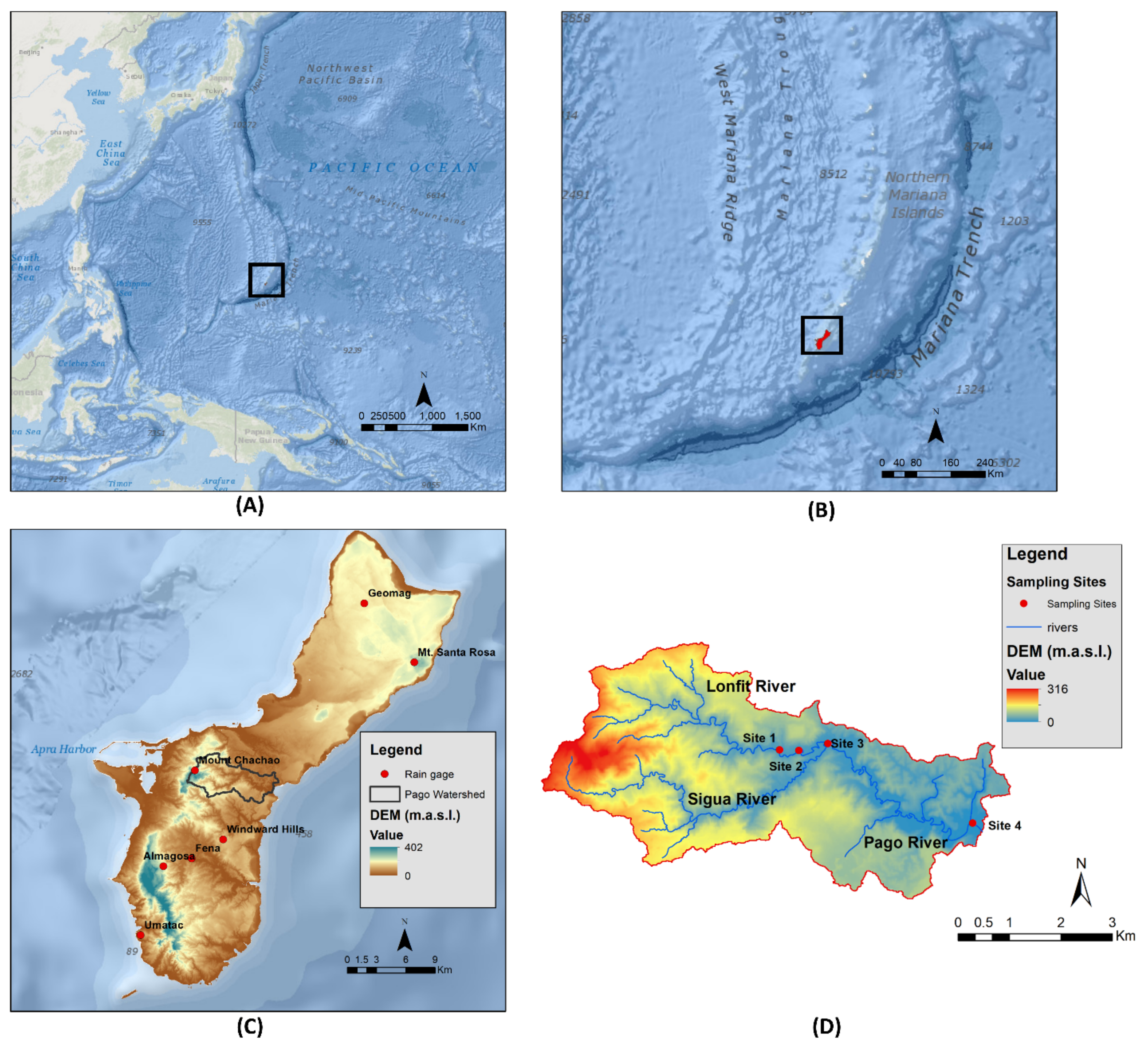
2.1. Study Area and Data

The Pago Watershed is located in the east of central Guam. It comprises three main channels: Longfit, Sigua, and Pago rivers, with a length of 8.08 km, 9.54 km, and 6.69 km, respectively. The drainage of the watershed is 23.41 km². The watershed elevation ranges from 0 m to 316 m (Figure 1).

Table 1. Geological information on the water sampling sites and observed data (rain gauges, and temperature, and streamflow).

	Sites	Latitude (°N)	Longitude (°N)	Elevation (m.a.s.l.)
Water sampling	Site 1	13.436	144.747	17
	Site 2	13.436	144.751	16
	Site 3	13.437	144.756	14
	Site 4	13.423	144.782	1
Rain gages	Mount Chachao	13.439	144.712	253
	Umatac	13.291	144.662	55
	Almagosa	13.353	144.683	183
	Fena	13.360	144.709	21
	Windward Hills	13.377	144.738	111
	Mt. Santa Rosa	13.536	144.914	253
	Geomag	13.589	144.868	145
Temperature	Antonio B. Won Pat Int. AP	13.453	144.767	22

shows geological information about the water sampling sites and stations measuring precipitation, temperature, and streamflow. Approximately 93.2 % of the total watershed area is vegetated, and half of the whole area consists of short bushes and grass (

Table 2. Land use of the Pago Watershed.

Land Uses	Area (ha)	Percent (%)
Range Grasses	1162.88	49.68
Forest Evergreen	972.71	41.55
Range Brush	138.57	5.92
Wetlands Forested	46.05	1.97
Residential Low Density	20.60	0.88

). The study area is composed of various volcanic and sediment clay types (Agfayan-Akina silty clay and Akina-Badland clay) and a clay-rock complex, as shown in

Table 3. Soil types of the Pago Watershed.

Soils	Slope Condition	Area (ha)	Percent (%)
Agfayan-Akina association	extremely steep	957.83	40.92
Agfayan-Akina-Rock outcrop association	extremely steep	525.02	22.43
Akina-Badland complex	15 to 30 percent slopes	514.98	22.00
Akina-Badland complex	7 to 15 percent slopes	126.58	5.41
Pulantat clay	30 to 60 percent slopes	93.73	4.00
Inarajan clay	0 to 4 percent slopes	51.43	2.20
Sasalaguan clay	7 to 15 percent slopes	24.65	1.05
Ritidian-Rock outcrop complex	15 to 60 percent slopes	20.97	0.90
Pulantat clay	7 to 15 percent slopes	12.87	0.55
Akina-Atate silty clays	7 to 15 percent slopes	11.15	0.48
Togcha-Ylig complex	3 to 7 percent slopes	1.60	0.07

.

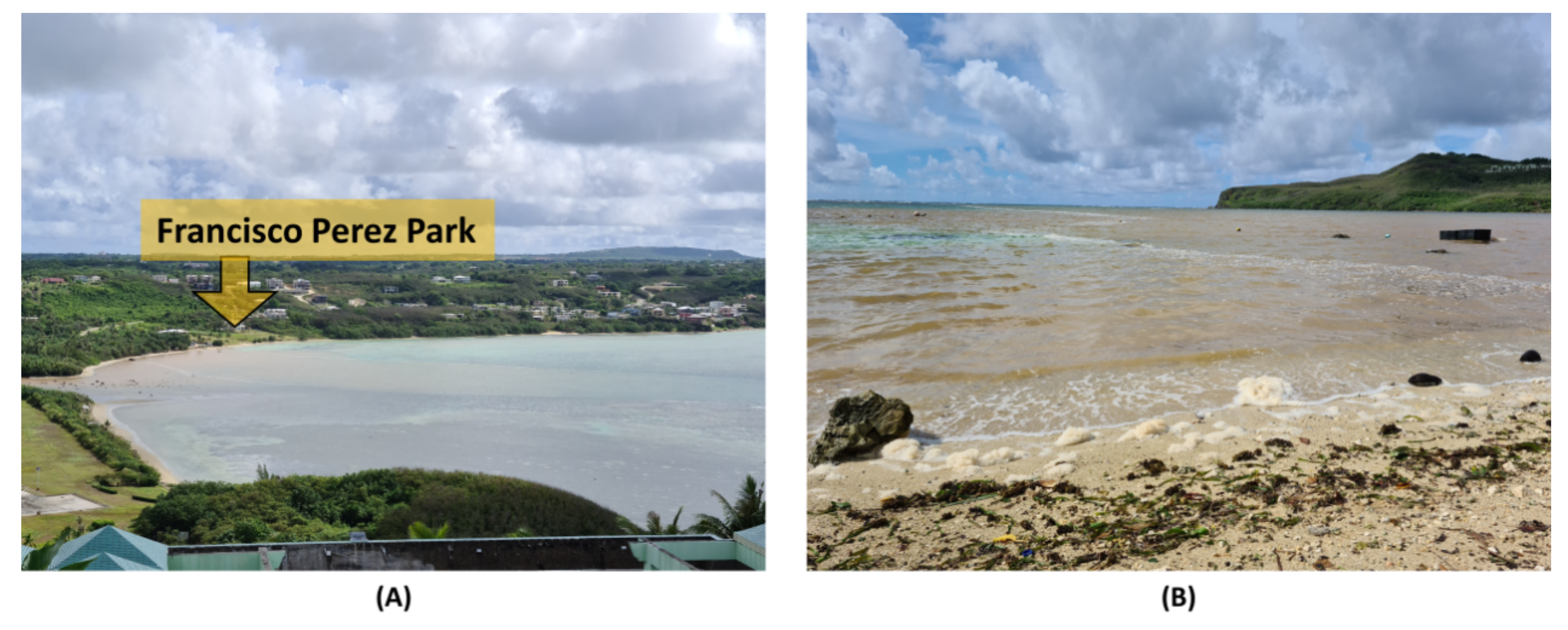
2.2. Experimental Approach: Water Quality Test

Sampling sites are determined by the end point of Longfit River, the start point of Pago River, and the Pago River mouth. Water samples are collected from two sites (upstream and downstream of Ordot Landfill) on Longfit River. Since the end and start points of Longfit and Pago rivers are within close proximity of one another, it is possible to estimate hydrologic variables and water quality information from Sigua River based on the law of conservation of mass. Figure 2 shows photos of the sampling sites under normal conditions. Water sampling has been conducted two times per week for a 9-week period (9 June 2021–4 August 2021). The additional sampling is performed to investigate storm implications on water quality by comparing water quality data from before and after storms. Since Site 1 and 2 are situated in the jungle, water sampling activity is done only at Site 3 and 4 under heavy rain conditions, due to safety concerns and accessibility. In this study, two water quality tests on dissolved inorganic nitrogen (IDN; nitrate and nitrite) and turbidity have been done.

2.3. Numerical Approach: SWAT Model

Various geospatial data are used in the SWAT model development. A 10 m ⨯ 10 m digital elevation model (DEM), obtained from Guam Coastal and Marine Spatial Planning (CMSP; https://www.oc.nps.edu/CMSP/Guam/ (accessed on 25 November 2021)), is used for delineating sub-basins within the Pago Watershed. In this study, soil data, from the Soil Survey Geographic Database (SSURGO), is collected from the Web Soil Survey, supported by the United States Department of Agriculture Natural Resources Conservation Service (USDA-NRCS; https://websoilsurvey.sc.egov.usda.gov/App/WebSoilSurvey.aspx (accessed on 25 November 2021)). The present study uses the land cover/use map generated in 2011 by the National Oceanic and Atmospheric Administration (NOAA) Coastal Change Analysis Program (C-CAP) (http://south.hydroguam.net/map-landcover-detailed-2011.php (accessed on 25 November 2021)).

Historical precipitation and temperature data are obtained from six rain gage stations and one temperature station (Table 1). These datasets have been recorded every 15 min since 2007 by the United States Geological Survey (USGS). Based on limited data availability caused by missing values, the period of 2012–2020 is used for a SWAT model development in this study. Other weather information, such as relative humidity, solar radiation, and wind speed, are estimated by a weather generator rendered using ArcSWAT. In addition to weather information, USGS has been measuring 15-min discharge rates below the confluence of Longfit and Sigua rivers to avoid measurement errors induced by the backflow of tides (see Figure 1). Data from this station (Pago River station; 16,865,000) are used for calibration and validation of a SWAT model.

In this study, ArcSWAT 2012 interface is used in building a SWAT model for the Pago Watershed. The watershed is divided into 11 sub-basins with 72 hydrologic response units (HRUs) based on the combination of slopes, land covers, and soil types (see Figure 3). After conducting a daily simulation, the estimated input daily discharge series to the Subbasin 4 is compared to the historical records from the USGS Pago River Streamflow station. The initial Nash-Sutcliffe efficiency (NSE) value and correlation coefficient value are 0.487 and 0.907, respectively.

The Sequential Uncertainty Fitting (SUFI2) method, one of the parameter methods of the SWAT-Calibration Uncertainty Program (SWAT-CUP), is implemented for calibrating parameters used in the SWAT model, and for conducting a global sensitivity analysis. The simulation period is divided into two periods: calibration (2012–2018), and validation periods (2019–2020).

3. Results and Discussion

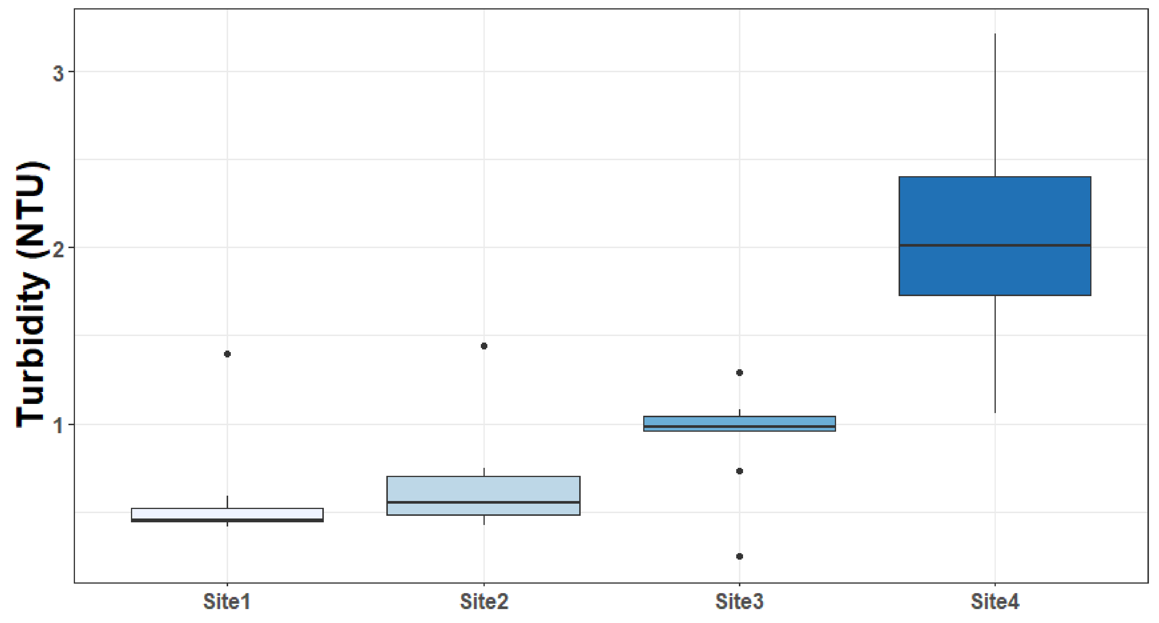
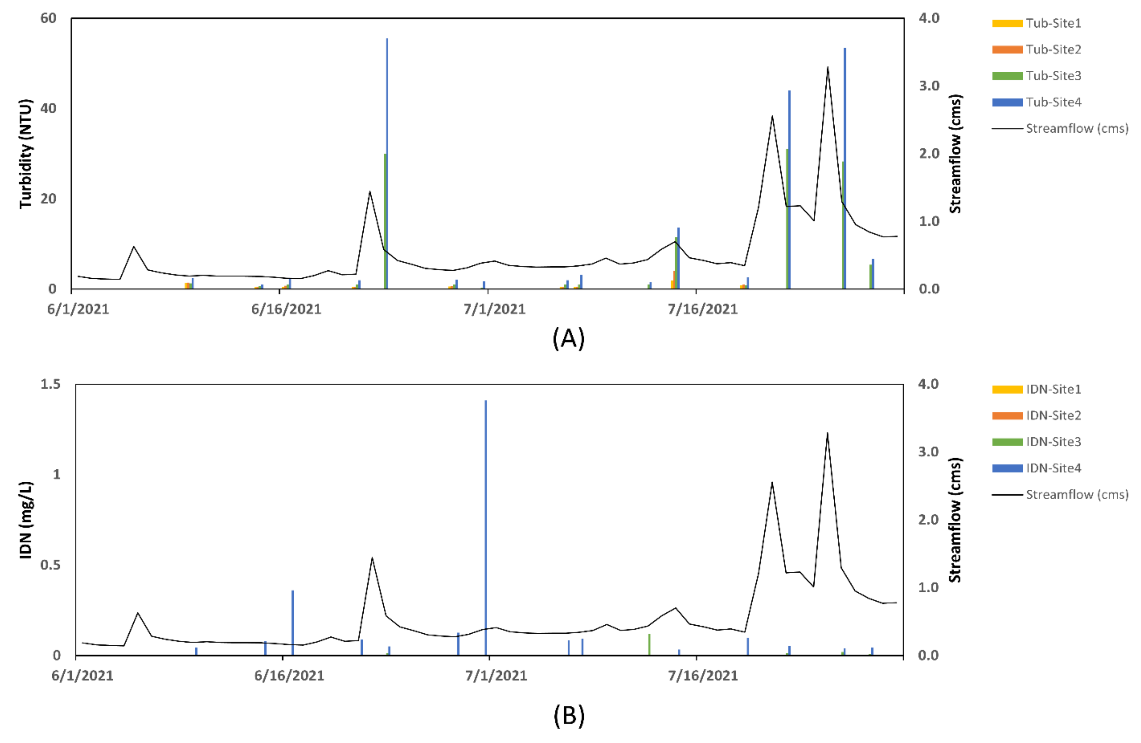
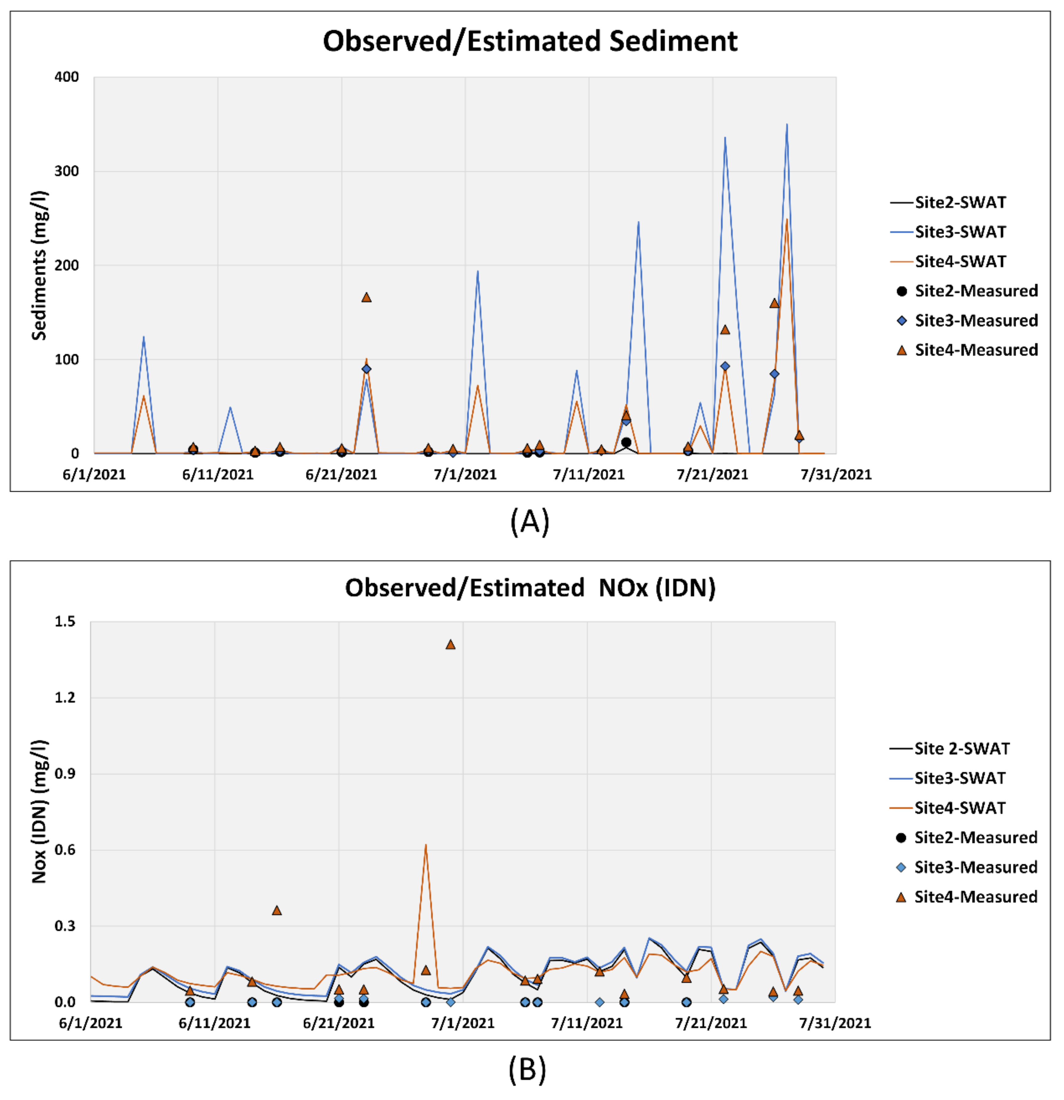
3.1. Water Quality Tests

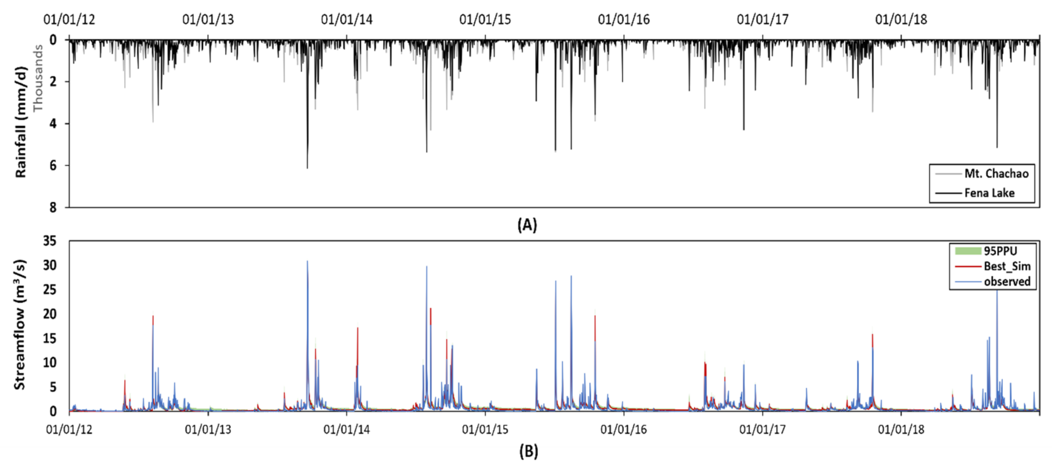
Dissolved inorganic nitrogen (nitrate and nitrite) and turbidity have been tested from the selected sites for the nine-week period of 9 June–4 August. As the wet monsoon season generally begins between July and August on Guam, the sampling period encompasses the end of the dry monsoon, the transition period, and the start of the wet monsoon. The water quality test results identify clear evidence of how storm and heavy rainfall contribute to erosion and sediments leading from the study area. Figure 4 shows photos taken from two sites (Site 3 and Site 4) at different times: dry-monsoon conditions, tropical depression conditions, and wet-monsoon conditions. Tropical Depression 06W hit Guam on 22 June 2021. Subsequently, the sampling activity was carried out the next day, 23 June 2021. While collecting water samples, photos were taken from Pago Bay Overlook and Francisco Perez Park (Figure 5) in order to account for the silt and nutrients transport phenomena within the Pago Bay coral reef area. It is evident that the silty freshwater had spread along the coast, as high sea level prevented the freshwater from draining directly into the ocean (Figure 5A). Sea foam was clearly found at the border between the seawater and river water (Figure 5B). This implies that the high concentration of dissolved organic matters is transported due to the peak discharge induced by heavy rainfalls.

Statistical analyses were carried out for identifying the location of most concern in relation to water quality aggravation. Since heavy rainfall disrupts the hydrological system within the watershed, an Analysis of Variance (ANOVA) test was implemented only on the data collected under dry-day conditions. From the one-way ANOVA test conducted, it was found that there were statistically significant differences in group means of turbidity (F value = 20.4 and p-value 3.29 × 10⁻⁷). Tukey’s honestly significant difference test (HSD), which was implemented for the multiple comparison procedure, identified that turbidity at Site 4 was statistically different from the other sites (see Figure 6). In addition to the turbidity tests, IDN concentrations at the first three sites were under detection limit. It has, therefore, been concluded that the target stressors are highly likely to be released significantly from Pago River.

Figure 7 shows the measured streamflow rates, turbidity, and IDN values for the project period of 1 June–4 August 2021. Streamflow data shown in this figure was collected from the USGS Pago River station (16,865,000; Site 3), and other water quality values were from each sampling site. To avoid safety issues, water sampling activities were performed the day after extreme rainfall occurred. Turbidity was highly related to the streamflow discharge rate (shown in Figure 7A), while the relationship between nitrate/nitrite concentrations and discharge was not observed (Figure 7B). Moreover, the turbidity values at Site 4 were always higher than those at Site 3, especially after heavy rainfall events. The implication is that some locations between Site 3 and Site 4 (the Pago River section) may contribute to sedimentation induced by erosion to Pago Bay.

3.2. SWAT Modeling

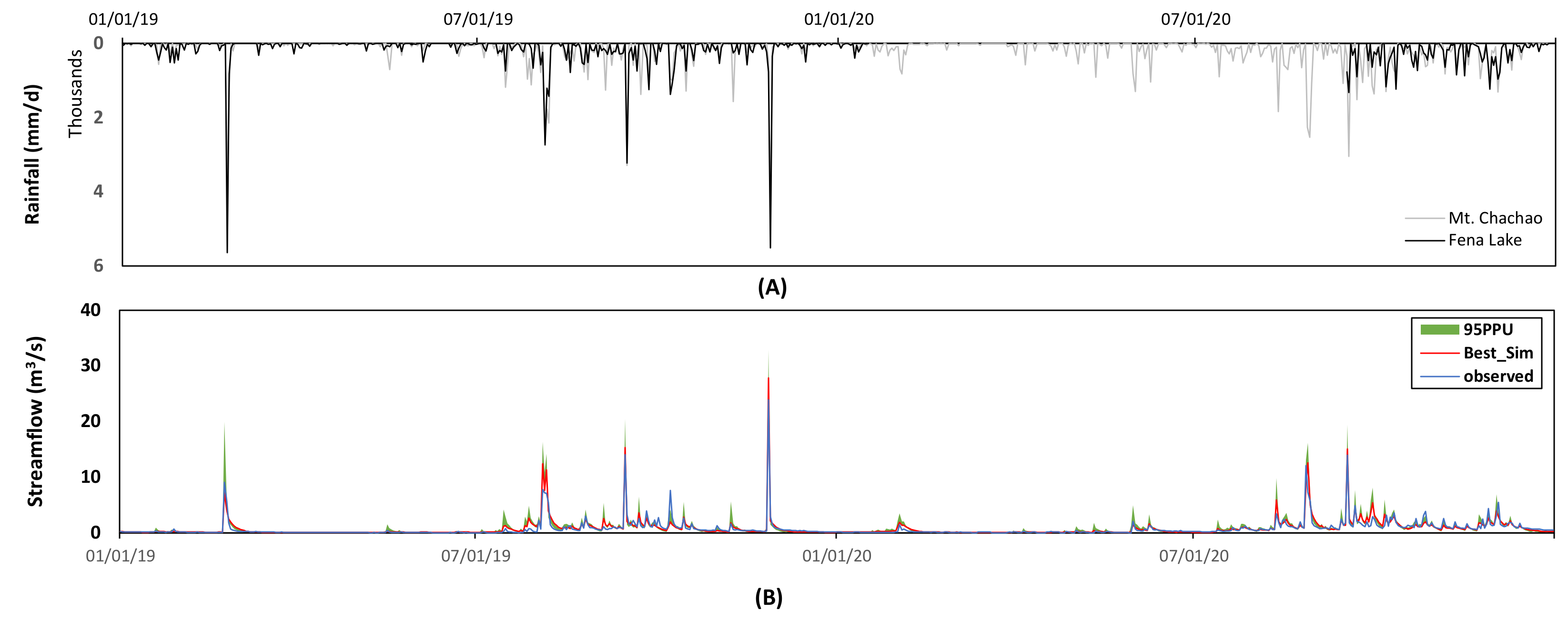
3.2.1. Model Performance and Sensitivity Analysis

The sensitivity analysis is carried out through 500 simulations using the SUFI2 method embedded in SWAT-CUP based on the maximum NSE value. The significant level (α) in this study is set to 0.05;

Table 4. SWAT model’s parameter sensitivity analysis results, best fitted value, and range.

Parameter Name	Description	t-Stat	p-Value	Fitted Value	Range
V__CN2.mgt	SCS runoff curve number	−88.31	0.00	80.31	80.01–97.66
V__CH_K2.rte	Effective hydraulic conductivity in the main channel	37.31	0.00	78.34	48.8–84.1
V__ALPHA_BF.gw	Baseflow alpha factor (days)	−14.76	0.00	0.32	0.31–0.46
R__SOL_K.sol	Saturated hydraulic conductivity	−3.25	0.00	0.43	0.18–0.61
V__SOL_AWC.sol	Soil water available capacity	1.79	0.07	0.16	0.15–0.17
V__ESCO.hru	Soil evaporation compensation factor	−1.67	0.10	0.35	0.18–0.38
V__GW_DELAY.gw	Groundwater delay (days)	1.65	0.10	459	419–478
V__GWQMN.gw	Minimum depth for ground water flow occurrence (mm)	1.62	0.11	1275	1233–1308
V__CH_N2.rte	Channel Manning’s roughness coefficient	0.98	0.33	0.17	0.16–0.19
R__SOL_BD.sol	Moist bulk density	−0.95	0.34	0.01	−0.05–0.02
V__GW_REVAP.gw	Groundwater revap coefficient	0.72	0.47	0.05	0.04–0.05
V__EPCO.bsn	Plant transpiration compensation factor	−0.69	0.49	0.92	0.88–0.94
R__OV_N.hru	Manning’s “n” value for overland flow	0.35	0.73	0.09	0.07–0.1

Note: Letter V denotes the replacement during the SUFI2 parameter procedure, and letter R the relative change.

shows that CN2, CH_K2, ALPHA_BF, and SOL_K are the most sensitive parameters of hydrologic processes within the Pago Watershed. With the calibrated values, daily streamflow is estimated for each subbasin. The NSE values are 0.864 and 0.857 for the calibration and validation periods, respectively. The R² value for the calibration period is 0.938, and the value for the validation period is 0.937. Figure 8 illustrates the graphical comparison of the observed and calibrated daily streamflows at the USGS Pago River stream gauge station for the calibration period. The estimated 95% uncertainties using the calibrated parameter ranges are shown in Figure 8 and Figure 9. The observed streamflow values fall into the uncertainty range under wet-conditions, while base flow values under dry-conditions are out of range. In addition to the comparison of the estimated streamflow, Figure 10 shows the measured and estimated sediments and IDN concentrations. The Alberta Transportation turbidity specification is used for converting the measured Nephelometric Turbidity Units (NTU) to total suspended solids (TSS). The calibration procedure using the SWAT-CUP is conducted using only historical streamflow rates at Site 3, as Guam does not have enough consecutive water quality records, such as sediments and IDN, like other small Pacific islands. As a result, the comparison of the estimated and measured values shows that the SWAT model is found to need to be improved for the sediments and nutrients.

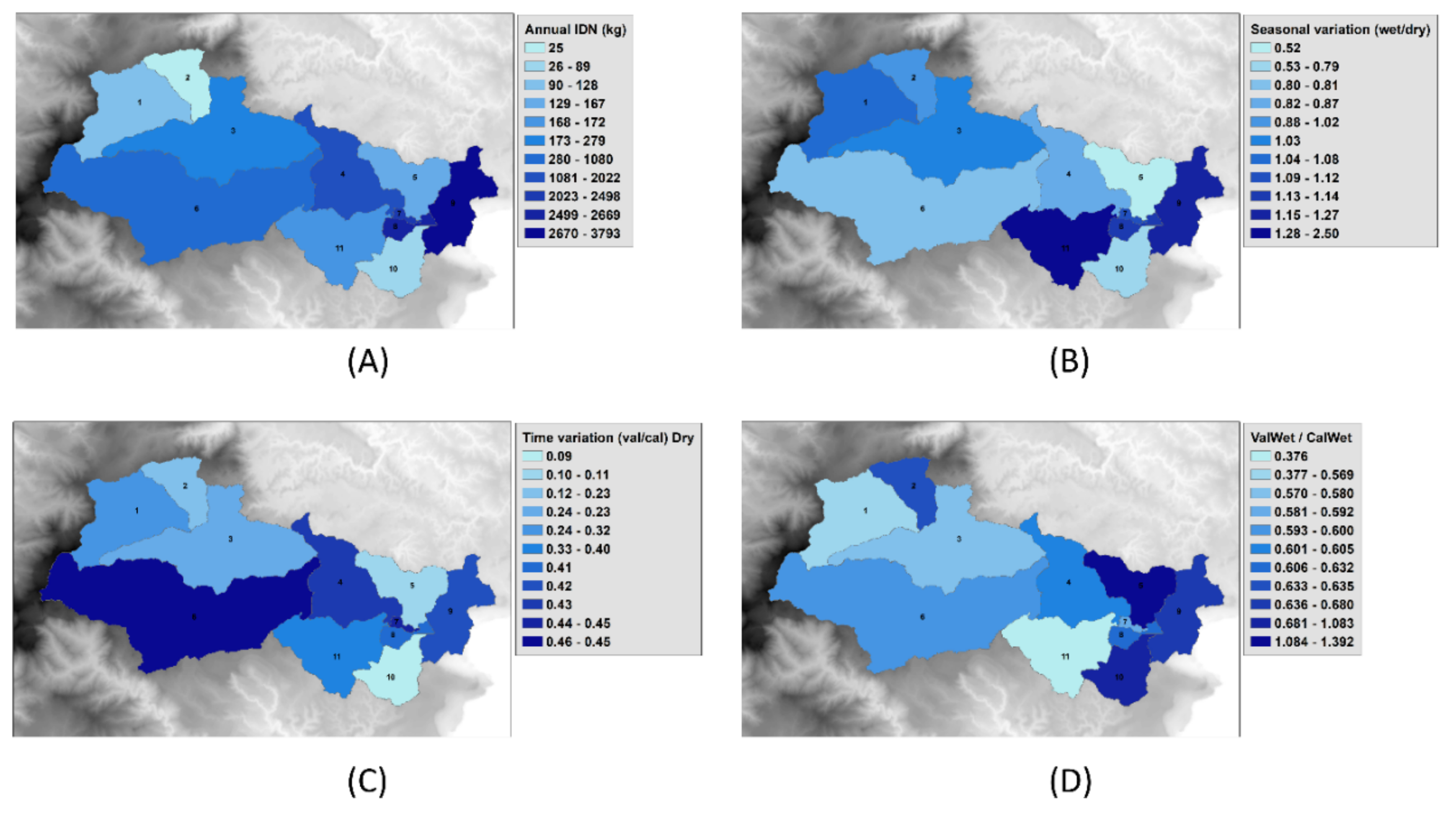
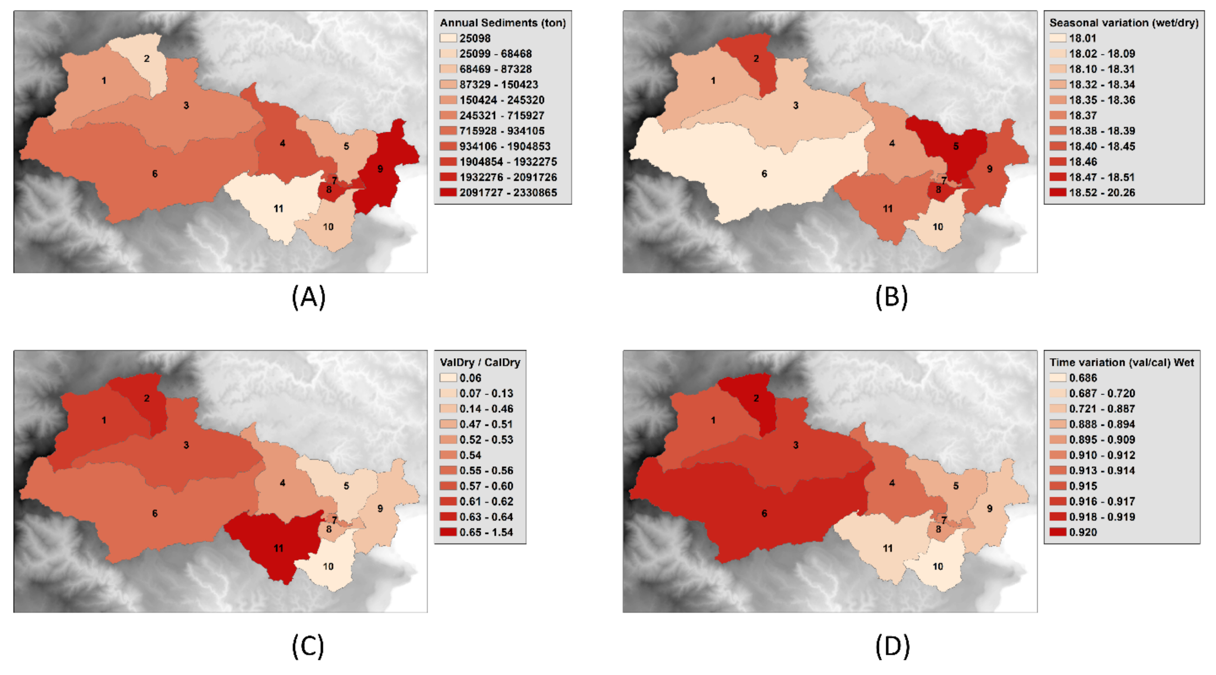
3.2.2. Identification of Sediment and IDN Source Area

Figure 11 shows how each sub-basin contributes to sediment loads, with respect to various time scales. The Pago River section (sub-basin 4, 7, 8, and 9) produces more sediments compared to other sub-basins, based on the annual total sediment loading map (Figure 11A), while sub-basins 2, 5, and 8 are most vulnerable to heavy rainfalls, based on the seasonal variation results which show these sub-basins to have the highest values (Figure 11B). Figure 11C,D illustrate time variation ratios comparing the sediments values of validation period to those of calibration period for dry and wet periods, respectively. Overall, the sediment loads show a reduced rate, with the exception of sub-basin 11 for the dry season.

Figure 12 shows the annual and seasonal variation of the IDN concentrations from sub-basins. Similarly, based on the annual total sediment loads, the Pago River section contributes high nitrogen concentration into the river flow. As shown in Figure 12B, sub-basins 7, 8, 9, and 11 produce larger amounts of inorganic nitrogen during the wet-monsoon period than any other sub-basins contributing to the inorganic nitrogen concentration during the dry-monsoon period. Similar to the time variation comparison of sediments, only sub-basins 2, 5, 9, and 10 yield more nitrogen amount for the validation period than for the calibration period.

Based on Figure 11A,B, and Figure 12A,B, it may be concluded that the Pago River area (sub-basins 4, 5, 7, 8, 9, 10, and 11) aggravates water quality within the Pago Watershed. Since Site 3 is situated at the starting point of sub-basin 4, the SWAT modeling outputs are consistent with the experimental water quality analyses.

4. Conclusions

Guam’s coral reefs and coastal environment have become more vulnerable due to identified threats, such as coastal development and pollution, recreational use and misuse, and increased climate change forcing disturbances. Creating impervious surfaces, applying fertilizers and pesticides, disposing of grease and oil to the aqua system without treatment, and the clearing of vegetation can accelerate terrestrial runoff of sediments and associated biological/chemical contaminants from uplands to coastal areas. Moreover, heavy rainfall accompanying storms increases runoff and terrestrially derived inputs of suspended solids, nutrients, and dissolved organic carbon, in turn increasing turbidity, eutrophication, and brownification. However, Pacific islands, including Guam, do not have enough measurement systems and historical records to account for the locations of concern. This study introduces the application of a SWAT model to support a ridge-to-reef management, which identifies vulnerable areas affecting coastal environments.

In this study, experimental and numerical approaches were implemented to discover which locations contribute to sediments and inorganic dissolved nitrogen concentrations. Water samples were collected from four sites (two on Longfit River, one at the starting point of Pago River, and the Pago River estuary) during a continuous 9-week period two times per week. ANOVA test and ad hoc analysis indicated that sediment loads from the Pago River section were significantly higher than those from other locations. After heavy rainfall events over the region, sea foam formation was observed, and may indicate high concentration of nutrients in the Pago coral reef area. In supporting the limits of the experimental approach, a SWAT model containing 11 sub-basins was developed for the watershed. The model was calibrated (2012–2018) and validated (2019–2020) using only historical streamflow records (2012–2020), measured at the USGS Pago River station located in Site 3. With SWAT-CUP application, the NSE values are 0.864 and 0.857 for the calibration and validation periods, respectively. The R² value for the calibration period is 0.938, and the value for the validation period is 0.937. Although it is found that the SWAT model needs to be improved further, it is consistent with experimental results which show that the Pago River section contributes significant amounts of sedimentation and IDN concentration to the Pago coral reef area.

In conclusion, two approaches applied in this study provide evidence that Pago River yields more sediments and nutrients than the other two rivers (Lonfit River and Sigua River) in the same riverflow system. The SWAT model’s results would allow local government agencies and Guam Environmental Protection Agency (EPA) to advance coral-reef conservation goals. The application of the SWAT model assists in rendering best management practices, particularly in controlling the total loads from point and non-point sources over locations where hydrological variables are rare, such as Guam. Subsequent work will combine climate change and land development scenarios to the developed SWAT model for accounting the effects of land use change and/or climate change on hydrologic processes over the region and the connected coral reef area.

References

1. Bartley, R.; Bainbridge, Z.T.; Lewis, S.E.; Kroon, F.J.; Wilkinson, S.N.; Brodie, J.E.; Silburn, D.M. Relating sediment impacts on coral reefs to watershed sources, processes and management: A review. Sci. Total Environ. 2014, 468, 1138–1153. [Google Scholar] [CrossRef] [PubMed]
2. Golbuu, Y.; van Woesik, R.; Richmond, R.H.; Harrison, P.; Fabricius, K.E. River discharge reduces reef coral diversity in Palau. Mar. Pollut. Bull. 2011, 62, 824–831. [Google Scholar] [CrossRef] [PubMed]
3. Uthicke, S.; Patel, F.; Ditchburn, R. Elevated land runoff after European settlement perturbs persistent foraminiferal assemblages on the Great Barrier Reef. Ecology 2012, 93, 111–121. [Google Scholar] [CrossRef] [PubMed]
4. Wolanski, E.; Martinez, J.A.; Richmond, R.H. Quantifying the impact of watershed urbanization on a coral reef: Maunalua Bay, Hawaii. Estuar. Coast. Shelf Sci. 2009, 84, 259–268. [Google Scholar] [CrossRef]
5. Comeros-Raynal, M.T.; Lawrence, A.; Sudek, M.; Vaeoso, M.; McGuire, K.; Regis, J.; Houk, P. Applying a ridge-to-reef framework to support watershed, water quality, and community-based fisheries management in American Samoa. Coral Reefs 2019, 38, 505–520. [Google Scholar] [CrossRef]
6. Guam Coral Reef Initiative. Guam Coral Reef Resilience Strategy; Guam Coral Reef Initiative: Washington, DC, USA, 2018; p. 69. [Google Scholar]
7. Smith, J.E.; Hunter, C.L.; Smith, C.M. The effects of top–down versus bottom–up control on benthic coral reef community structure. Oecologia 2010, 163, 497–507. [Google Scholar] [CrossRef] [PubMed]
8. Delevaux, J.; Winter, K.B.; Jupiter, S.D.; Blaich-Vaughan, M.; Stamoulis, K.A.; Bremer, L.L.; Burnett, K.; Garrod, P.; Troller, J.L.; Ticktin, T. Linking land and sea through collaborative research to inform contemporary applications of traditional resource management in Hawai’i. Sustainability 2018, 10, 3147. [Google Scholar] [CrossRef] [Green Version]
9. Carlson, R.R.; Foo, S.A.; Asner, G.P. Land use impacts on coral reef health: A ridge-to-reef perspective. Front. Mar. Sci. 2019, 6, 562. [Google Scholar] [CrossRef]
10. Delevaux, J.; Stamoulis, K. Assessment of Ridge-to-Reef Management; Seascape Solutions LLC: Portsmouth, NH, USA, 2020. [Google Scholar]
11. Leta, O.T.; El-Kadi, A.I.; Dulai, H.; Ghazal, K.A. Assessment of SWAT model performance in simulating daily streamflow under rainfall data scarcity in Pacific island watersheds. Water 2018, 10, 1533. [Google Scholar] [CrossRef] [Green Version]
12. Mukundan, R.; Hoang, L.; Gelda, R.K.; Yeo, M.-H.; Owens, E.M. Climate change impact on nutrient loading in a water supply watershed. J. Hydrol. 2020, 586, 124868. [Google Scholar] [CrossRef]
13. Ricci, G.F.; De Girolamo, A.M.; Abdelwahab, O.M.; Gentile, F. Identifying sediment source areas in a Mediterranean watershed using the SWAT model. Land Degrad. Dev. 2018, 29, 1233–1248. [Google Scholar] [CrossRef]
14. Betrie, G.D.; Mohamed, Y.A.; Griensven, A.V.; Srinivasan, R. Sediment management modelling in the Blue Nile Basin using SWAT model. Hydrol. Earth Syst. Sci. 2011, 15, 807–818. [Google Scholar] [CrossRef] [Green Version]
15. Melaku, N.D.; Renschler, C.S.; Holzmann, H.; Strohmeier, S.; Bayu, W.; Zucca, C.; Ziadat, F.; Klik, A. Prediction of soil and water conservation structure impacts on runoff and erosion processes using SWAT model in the northern Ethiopian highlands. J. Soils Sedim. 2018, 18, 1743–1755. [Google Scholar] [CrossRef] [Green Version]
16. Yang, K.; Lu, C. Evaluation of land-use change effects on runoff and soil erosion of a hilly basin—The Yanhe River in the Chinese Loess Plateau. Land Degrad. Dev. 2018, 29, 1211–1221. [Google Scholar] [CrossRef]
17. Paulay, G. Marine biodiversity of Guam and the Marianas: Overview. Micronesica 2003, 35, 3–25. [Google Scholar]
18. Burdick, D.; Brown, V.; Asher, J.; Caballes, C.; Gawel, M.; Goldman, L.; Hall, A.; Kenyon, J.; Leberer, T.; Lundblad, E. Status of the Coral Reef Ecosystems of Guam; University of Guam Marine Laboratory: Mangilao, GU, USA, 2008. [Google Scholar]
19. GVB. Annual Report: 2017; Guam Visitors Bureau: Tamuning, GU, USA, 2018; p. 65. [Google Scholar]
Figure 1. Geographical information on the study area (Pago Watershed) in Guam. (A) location of the island of Guam in the Pacific Ocean, (B) location of the island in the Mariana region, (C) location of the Pago Watershed in Guam, and (D) the study area which encompasses the Pago Watershed, including the Lonfit, Sigua, and Pago rivers. Red points denote the rain gages in (C) and sampling sites in (D) for water quality tests. Sources for World Ocean Reference and Bases in (AC) are Esri, GEBCO, NOAA, National Geographic, Garmin, HERE, Geonames.org, and other contributors.
Water 13 03351 g001
Figure 2. Photos for each sampling site. (A) upstream from Ordot Landfill, (B) downstream from Ordot Landfill, (C) USGS Pago River streamflow gauge, and (D) near Pago River mouth.
Water 13 03351 g002
Figure 3. Delineated 11 sub-basins.
Water 13 03351 g003
Figure 4. Site photos with respect to different sampling times. The top three photos were taken from Site 3, and the bottom three from Site 4. (A,D) were taken during a dry monsoon condition, (B,E) on 23 June 2021 (the day after Tropical Depression 06W), and (C,F) on 2 August 2021.
Water 13 03351 g004
Figure 5. Photos from Pago Bay Outlook (A) and Francisco Perez Park (B) on 23 June 2021, the day after Tropical Depression 06W made landfall on Guam.
Water 13 03351 g005
Figure 6. Boxplot for turbidity test results for the four sites.
Water 13 03351 g006
Figure 7. Observed streamflow at Site 3, and turbidity and IDN data at four sites for the project period (1 June–4 August). (A) turbidity values at four sites, (B) IDN values at four sites.
Water 13 03351 g007
Figure 8. (A) Daily measured rainfall data sets from Mt. Chachao and Fena Lake rain gauge stations, and (B) observed, simulated daily streamflows, and the estimated 95% model uncertainty at USGS Pago River station (16,865,000) for the calibration period (2012–2018).
Water 13 03351 g008
Figure 9. (A) Daily measured rainfall data sets from Mt. Chachao and Fena Lake rain gauge stations, and (B) observed, simulated daily streamflows, and the estimated 95% model uncertainty at USGS Pago River station (16,865,000) for the validation period (2019–2020).
Water 13 03351 g009
Figure 10. Comparison of the sediments (A) and IDN (B) estimated by the calibrated SWAT model with the measured values for the period of 1 June to 31 July 2021.
Water 13 03351 g010
Figure 11. Sediment contribution maps. (A) Average annual total sediments, (B) seasonal variation (ratio of wet to dry), (C) time variation (ratio of validation to calibration periods) for the dry season, and (D) time variation (ratio of validation to calibration.
Water 13 03351 g011
Figure 12. IDN contribution maps. (A) Average annual total sediments, (B) seasonal variation (ratio of wet to dry), (C) time variation (ratio of validation to calibration periods) for the dry season, and (D) time variation (ratio of validation to calibration periods) for the wet season.
Water 13 03351 g012