Vertical Distribution of Phytoplankton Community and Pigment Production in the Yellow Sea and the East China Sea during the Late Summer Season

Abstract

Phytoplankton community structure, which plays an important role in determining productivity and food web structure, can provide important information for understanding variations in marine ecosystems under projected climate change scenarios. Rising temperatures due to climate change will increase and intensify water stratification. To understand the community composition and distribution characteristics of phytoplankton under stratified conditions, phytoplankton pigments were analyzed in the Yellow Sea (YS) and East China Sea (ECS) during the late summer season. In addition, pigment production was measured to estimate the physiological characteristics of phytoplankton relating to light, which is an essential element of photosynthesis. During our observation period, no distinct differences were found in the community composition and pigment production of phytoplankton in the YS and the ECS, but differences in the vertical distribution were observed. Overall, the dominant phytoplankton classes at the surface depth were pico-sized cyanobacteria (46.1%), whereas micro- and nano-sized diatoms (42.9%) were the abundant most classes at a 1% light depth. The major factors controlling the vertical distributions of the phytoplankton community were temperature and nutrients (i.e., nitrate and ammonium). Cyanobacteria were positively correlated with water temperature and ammonium, whereas diatoms were negatively related to water temperature and positively correlated with nitrates. Based on the pigment production, it was found that cyanobacteria at the surface layer encountered excessive irradiance conditions during the study period. The productivity of the cyanobacterial community could be decreased under high-light and high-temperature conditions. This means that cyanobacteria could have a negative influence on the quantity and quality of food available to upper trophic organisms under warmer conditions.

1. Introduction

Phytoplankton, one of the main primary producers, plays a key role in the aquatic food web and the biogeochemical cycle. Since the biomass and community structure of phytoplankton are directly affected by the physical and chemical properties of ambient water [1,2], future scenarios for phytoplankton change in marine ecosystems are matters of great concern under the ongoing conditions of climate change [3,4,5]. Increasing water stratification in the oceans is likely to lead to nutrient-deficient conditions, decreased biomass, and selection for smaller cells [3,6,7]. These environmental variations, especially in cell size, largely affect the quantity and quality of food sources [8]. In addition, completely different food web structures can be found by dominant species compositions and groups even among phytoplankton species of similar sizes [9]. Thus, studying the phytoplankton community structure is important in order to understand potential ecosystem responses to global climate change.

Light, which is essential for photosynthetic activity, is one of the main environmental variables affected by water stratification. Phytoplankton change their pigment pool to cope with fluctuating light conditions. In general, smaller phytoplankton species tend to have higher intracellular pigments than larger species, which enables smaller phytoplankton to grow better under low-light conditions [10,11]. When phytoplankton are exposed to strong light and ultraviolet radiation, they produce and accumulate photoprotective pigments [12,13]. Therefore, phytoplankton pigments are believed to provide important clues about the physiological status of each phytoplankton species through the different light regimes that are closely related to photosynthesis.

The Yellow Sea (YS) is a shallow semi-enclosed marginal sea (20–90 m) in the western Pacific Ocean surrounded by Korea and China. There is a strong water stratification in the central YS due to a combination of weak winds and strong solar irradiance during the late spring-early autumn period [14]. As a result, distinct distribution characteristics in terms of nutrients, phytoplankton biomass, and size-fraction structure have been observed in the central YS [15,16]. The East China Sea (ECS) is the largest marginal sea with a wide continental shelf that is affected by the nutrient-sufficient freshwater of the Changjiang River and the subtropical open-ocean waters of the Kuroshio Current [17]. The different environmental dynamics of the ECS over the seasons result in high variations in the biomass, community structure, and primary production of phytoplankton [18]. Thus, studies on the spatial characteristics of phytoplankton with regard to community compositions and pigment production were carried out based on the unique environmental properties of the YS and ECS, especially in the summer season. In this study, our primary objective was to identify the major factors that influence the vertical distribution of the phytoplankton community in the study area. Our other objective was to identify the photophysiological traits of phytoplankton in the YS and ECS.

2. Materials and Methods

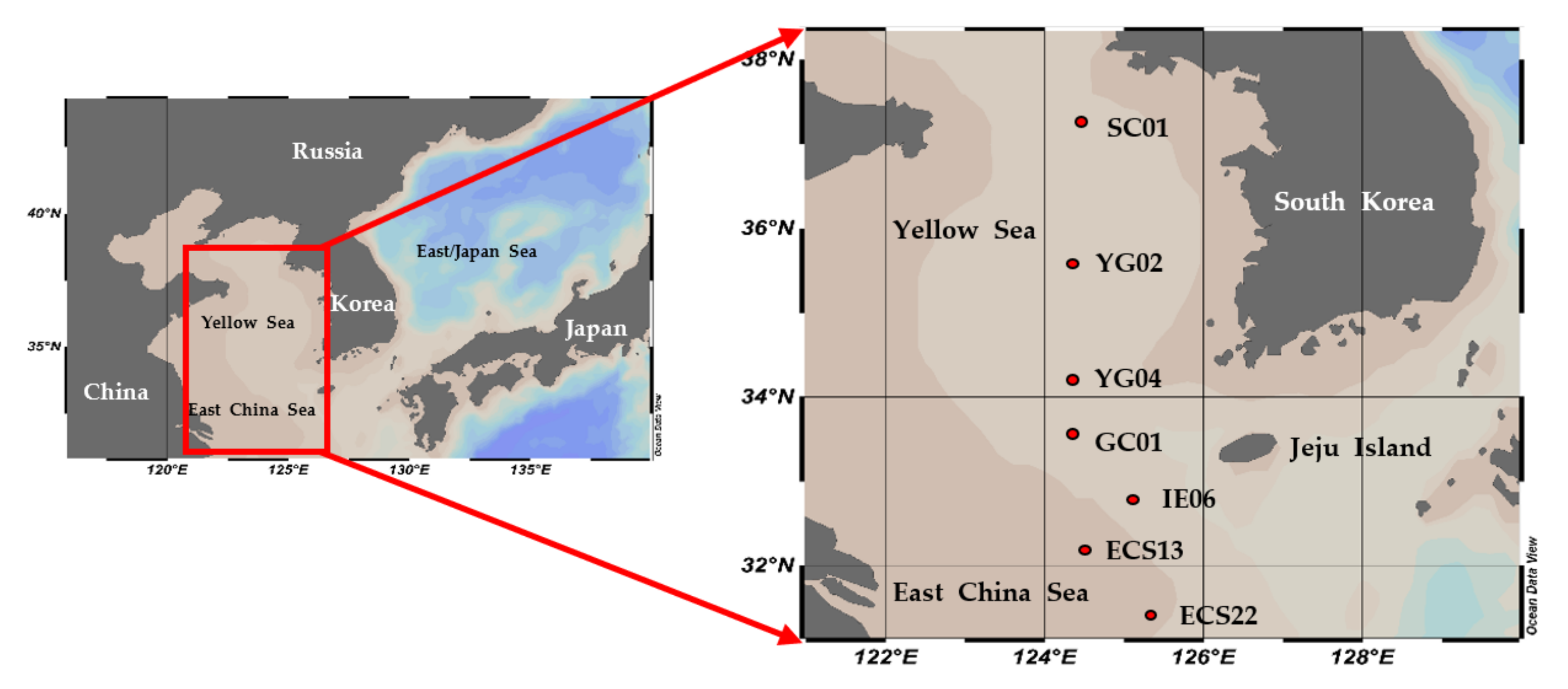
2.1. Sample Collection and Environmental Data

Sampling was carried out at seven stations in the YS (four stations) and ECS (three stations) during late summer (9–13 September) 2020 on board the R/V Onnuri (Figure 1 and

Table 1. Station information and environmental condition in the YS and the ECS during the late summer of 2020.

Region	Station	Date (2020)	Latitude (°N)	Longitude (°E)	Mixed Layer Depth (m)	Stability Index	Light Depth (%)	Depth (m)	T (°C)	S (psu)	NO3 (µM)	NH4 (µM)
Yellow Sea (YS)	SC01	13-Sep	31.400	125.330	21	0.068	100	0	21.7	31.2	0.18	1.00
							1	30	16.0	31.9	5.12	0.96
	YG02	12-Sep	32.175	124.510	10	0.055	100	0	24.2	31.5	1.05	0.83
							1	27	21.0	32.2	5.53	1.00
	YG04	12-Sep	32.771	125.108	15	0.096	100	0	23.2	30.8	3.76	1.45
							1	33	16.6	32.5	11.35	0.71
	GC01	12-Sep	33.565	124.353	13	0.094	100	0	23.4	30.9	2.06	1.54
							1	51	11.8	33.3	13.42	1.00
East China Sea (ECS)	IE06	11-Sep	34.195	124.352	12	0.025	100	0	24.8	30.5	2.33	1.29
							1	19	23.8	30.6	5.90	1.08
	ECS13	10-Sep	35.556	124.349	12	0.065	100	0	25.9	30.2	0.80	0.79
							1	19	24.0	31.0	5.31	0.87
	ECS22	09-Sep	37.254	124.449	12	0.044	100	0	26.2	32.0	1.51	1.37
							1	41	24.6	33.5	6.33	1.04

). Physical data were obtained using a CTD (SBE 911 plus, Seabird Electronics Inc., Bellevue, WA). The mixed layer depth (MLD) was determined at each station based on a density difference of 0.125 σ_t from the surface layer [19,20], while the stability index of the euphotic zone was calculated based on [21]. Seawater samples were obtained from Niskin bottles attached to a CTD/rosette sampler to assess nitrogen sources (nitrate, NO₃; ammonium, NH₄) at two light depths (100% and 1% penetration depths of photosynthetically active radiation, PAR, at the surface). The samples were filtered through 0.7 µm GF/F filters (Whatman) for nutrient analysis and the filtered water samples were put into high-density polyethylene bottles (50 mL) that were stored at −20 °C for further analysis. In the home laboratory in Pusan National University, South Korea, the concentrations of nitrate and ammonium were analyzed using standard spectrophotometric methods [22].

2.2. Size-Fractionated Chlorophyll-a Measurement

Seawater samples of size-fractionated chlorophyll-a were collected at the two light depths (100% and 1% PAR penetration) at all the stations (total number of samples: 14). Each water sample (0.5 L) was passed sequentially through 20, 2, and then 0.7 µm filters to separate out micro- (>20 µm), nano- (2–20 µm), and pico-size (0.7–2 µm) phytoplankton, respectively [23,24]. The filters were wrapped in aluminum foil to prevent photolysis and stored in a freezer (−20 °C) in the laboratory for further analysis. The concentrations of the size-fractionated chlorophyll-a were analyzed using a precalibrated fluorometer (Turner Designs model 10-AU) based on the procedure of [25].

2.3. In Situ Culture Experiment for Photosynthetic Pigment Production

Seawater samples (4–5 L) used to assess the natural carbon-13 (¹³C) value of each photosynthetic pigment were filtered through 0.7 µm Whatman GF/F filter paper (47 mm) before the in situ culture experiments. The seawater samples (9 L) used for incubation were filtered through a 300 µm filter to eliminate zooplankton and detritus. The filtered water samples were transferred into large polycarbonate incubation bottles (9 L) covered with screens (LEE Filters, Andover, UK) corresponding to each light depth, then a labeled carbon (NaH¹³CO³, 99%) solution was added as a tracer [26,27]. The amount of ¹³C injected into the incubation bottle was determined by 10–15% of the total dissolved inorganic carbon concentration in the water sample [26,27]. The bottles were incubated in an acrylic incubator on deck that was cooled by circulating surface seawater under natural light conditions for 4 h [26,27]. After incubation, water samples from each bottle were filtered (>4 L) through GF/F filter papers (47 mm). The filters were wrapped with aluminum foil to prevent photolysis and kept frozen (−20 °C) until further analysis could take place.

2.4. Extraction and Analysis for Photosynthetic Pigment Production

The filter paper used for the pigment production was cut into small pieces to enhance the extraction efficiency [28], then small pieces of the filter were transferred to centrifuge tubes containing 100% acetone (3.5 mL) and canthaxanthin (100 µL; internal standard). Photosynthetic pigments from the sample in the centrifuge tube were extracted for 24 h in cool (4 °C) and dark conditions after sonification [29]. The extract was centrifuged and then the supernatant was passed through a 0.2 µm syringe filter (Advantec, Tokyo, Japan) for purification. The 3 mL purified extract was mixed with 0.9 mL of deionized water (1 mL sample: 0.3 mL deionized water, v:v). A further analysis of the extracted pigments was performed using high-performance liquid chromatography (HPLC) based on the method of [30]. Analyses were conducted on an Agilent Infinite 1260 HPLC system equipped with a Zobrax Eclipse XDB C8 (250 × 4.6 mm, 5 µm) column. Eluent A was a mixture of methanol:acetonitrile:aqueous pyridine (0.25 M pyridine) (50:25:25, v:v:v), while eluent B was a mixture of methanol:acetonitrile:acetone (20:60:20, v:v:v). The binary linear gradient profiles were adapted to separate pigments: 100:0 (A:B), 0 min; 60:40, 21 min; 5:95, 27 min; 5:95, 37 min; and 100:0, 45 min. Photosynthetic pigments were detected and quantified at 430 nm. The identification of each pigment was based on the retention time of authentic standards (DHI Water & Environment, Hørsholm, Denmark). The separated pigments were collected based on the retention time of each pigment using a HPLC fraction collector with a transparent glass vial (5 mL), including half of the Whatman GF/F filter paper (25 mm). The eluents from each collected photosynthetic pigment were removed by a nitrogen purge equipment and then the filter within the collection vial was wrapped with a tin cap to analyze the delta ¹³C value of each pigment at the University of Alaska Fairbanks, USA.

2.5. Calculation of the Pigment Concentration and Production Rate

The calculation of the photosynthetic pigment concentrations was based on chromatographic peak areas in compliance with the method developed by [31].

$$\mathrm{C}=\mathrm{Area}\times \mathrm{Rf}\times \frac{\mathrm{Ve}}{\mathrm{Vs}}$$

(1)

where C = pigment concentration (µg L^–1); Area = area of the peak (area); Rf = standard response factor (µg L^–1 area^–1); Ve = {AIS × volume of internal standard (I.S.) added to sample} ÷ peak area of the I.S. added to sample (L); AIS = peak area of the I.S. when 1 mL of I.S. is mixed with 300 µL of deionized water (area); Vs = volume of filtered water sample (L).

The equation used to calculate the pigment production rate was based on the method proposed by [27].

$$\Delta \mathrm{PPR}\left(\mathrm{t}\right)=\mathrm{PPR}\times \frac{a_{is}-a_{ns}}{a_{ic}-a_{ns}}$$

(2)

where ∆PPR = amount of each pigment carbon photosynthetically produced during the incubation; a_is = ¹³C atom % in each pigment compound of the incubated sample; a_ns = ¹³C atom % in each pigment compound of the natural sample; a_ic = ¹³C atom % in the ¹³C enriched inorganic carbon; PPR = carbon concentration of each pigment at the end of incubation.

2.6. Chemotaxonomic Analysis

The contributions of different phytoplankton classes to the total chlorophyll-a were calculated using the CHEMTAX software [32,33,34]. Eight phytoplankton groups were functionally defined according to their pigment contents: dinoflagellates, diatoms, chrysophytes, prymnesiophytes, chlorophytes, cryptophytes, prasinophytes, and cyanobacteria. The input pigment ratios matrix used in the CHEMTAX program were based on the pigment relationships of common phytoplankton groups adjacent to our study area [18,35].

3. Results

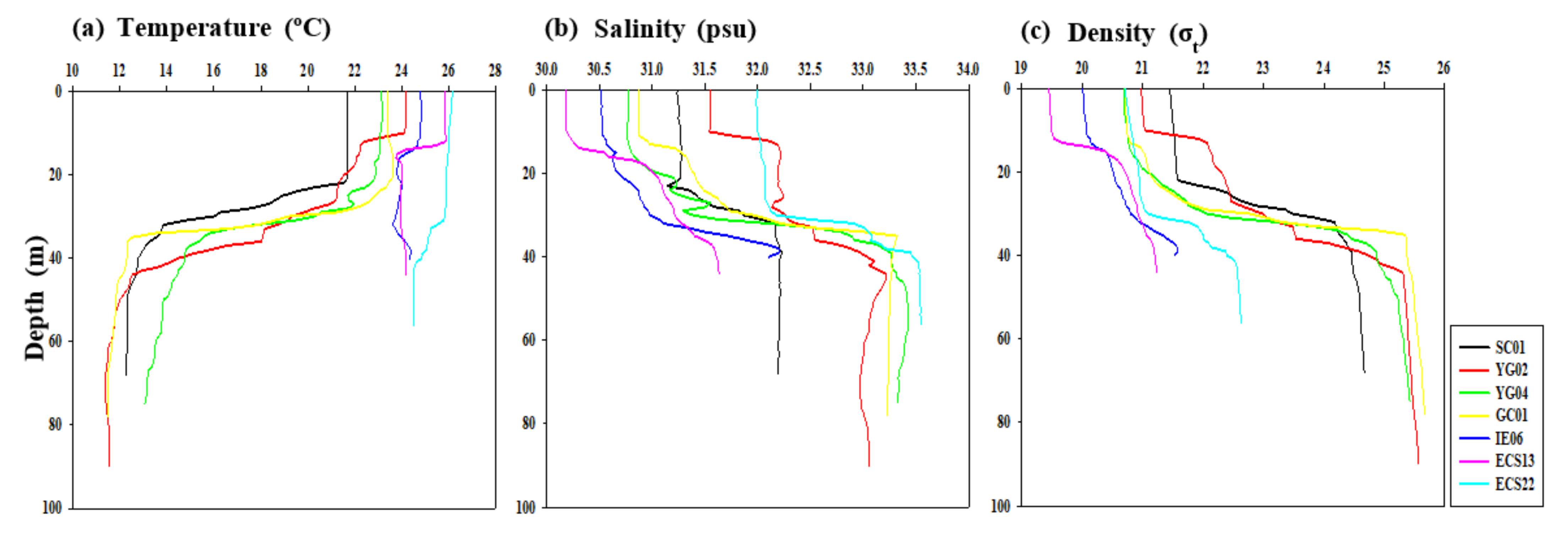
3.1. Environmental Conditions

The hydrographic conditions in the YS and the ECS are shown in Figure 2 and Table 1. The MLD at the YS stations ranged from 10 to 21 m with a mean of 15 m (S.D. = ±5 m), whereas all the ECS stations had identical MLDs (12 m). The average euphotic depth (i.e., the depth receiving 1% of the surface PAR) was 35 ± 11 m (mean ± S.D.; range = 27–51 m) and 26 ± 13 m (mean ± S.D.; range = 19–41 m) in the YS and the ECS, respectively. During our study period, the euphotic depths were relatively deeper than the MLDs at all stations (Table 1), which means that the water column in this study area was stratified by the density difference. The stratification intensity estimated from the stability index was relatively higher in the YS (mean ± S.D. = 0.078 ± 0.020) than in the ECS (mean ± S.D. = 0.044 ± 0.020) (Table 1). The water temperatures at the surface and bottom of the euphotic depth in the YS ranged from 21.7 to 24.2 °C (mean ± S.D. = 23.1 ± 1.0 °C) and 11.8 to 21.0 °C (mean ± S.D. = 16.3 ± 3.7 °C), respectively, whereas those of the ECS ranged from 21.7 to 24.2 °C (mean ± S.D. = 23.1 ± 1.0 °C) and 11.8 to 21.0 °C (mean ± S.D. = 16.3 ± 3.7 °C), respectively. The salinity of the YS at 100 and 1% light depths ranged from 30.8 to 31.5 psu (mean ± S.D. = 31.1 ± 0.4 psu) and 31.9 to 33.3 psu (mean ± S.D. = 32.4 ± 0.6 psu), respectively, whereas that of the ECS ranged from 30.2 to 32.0 psu (mean ± S.D. = 30.9 ± 1.0 psu) and 30.6 to 33.5 psu (mean ± S.D. = 31.7 ± 1.6 psu), respectively. Significant differences in water temperature (t-test, p < 0.05) and salinity (t-test, p < 0.01) between the surface layer and the 1% light depth were observed at the YS station, whereas the ECS only showed a significant difference in water temperature (t-test, p < 0.05) (Table 1).

The two nitrogen sources (NO₃ and NH₄) had different distribution patterns at 100 and 1% light depths during this study period. The NO₃ concentrations at all stations of the YS and the ECS were significantly higher at a 1% light depth (YS: range = 5.12–13.42 µM. mean ± S.D. = 8.85 ± 4.16 µM; ECS: range = 5.31–6.33 µM, mean ± S.D. = 5.85 ± 0.51 µM) than at the surface layer (YS: range = 0.18–3.76 µM, mean ± S.D. = 1.76 ± 1.54 µM; ECS: range = 0.80–2.33 µM, mean ± S.D. = 1.55 ± 0.76 µM), whereas no noticeable differences in NH₄ concentrations were found at both euphotic depths in the YS (100% light depth: range = 0.83–1.54 µM, mean ± S.D. = 1.21 ± 0.34 µM; 1% light depth: range = 0.71–1.00 µM, mean ± S.D. = 0.92 ± 0.14 µM) and the ECS (100% light depth: range = 0.79–1.37 µM, mean ± S.D. = 1.15 ± 0.31 µM; 1% light depth: range = 0.87–1.08 µM, mean ± S.D. = 1.00 ± 0.11 µM) (Table 1).

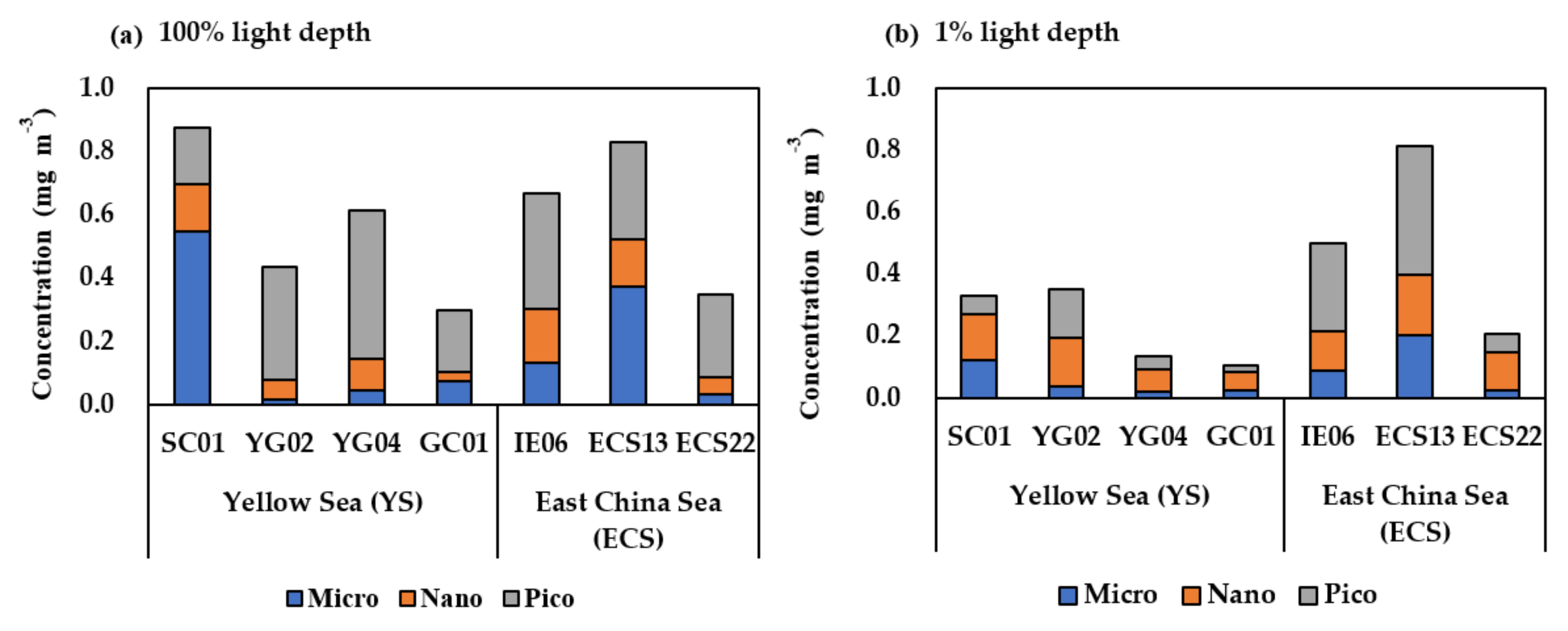
3.2. Total and Size-Fractionated Chlorophyll-a Concentration in the YS and the ECS

No distinct distribution patterns according to latitude were found for the total chlorophyll-a concentrations (sum of micro, nano, and pico-sized chlorophyll-a concentrations) at each light depth during our observation period (Figure 3). The average total chlorophyll-a concentration at the YS stations was 0.56 ± 0.25 mg m⁻³ (mean ± S.D.; range = 0.30–0.88 mg m⁻³) at a 100% light depth and 0.23 ± 0.13 mg m⁻³ (mean ± S.D.; range = 0.10–0.35 mg m⁻³) at a 1% light depth, whereas that of the ECS stations was 0.62 ± 0.25 mg m⁻³ (mean ± S.D.; range = 0.35–0.83 mg m⁻³) and 0.51 ± 0.31 mg m⁻³ (mean ± S.D.; range = 0.20–0.82 mg m⁻³) at a 100 and 1% light depth, respectively (Figure 3).

Overall, the phytoplankton size structure of both study regions at the surface layer was dominated by pico-sized phytoplankton, except for at two stations (SC01 and ECS13), which were dominated by micro-sized phytoplankton, whereas nano-sized phytoplankton had a relatively high biomass at a 1% light depth of the YS and the ECS (except for stations IE06 and ECS 13, where pico-sized phytoplankton were the dominant class) during late summer of 2020 (Figure 3). The average chlorophyll-a concentrations for micro-, nano-, and pico-sized phytoplankton at the surface layer of the YS stations were 0.17 ± 0.25 mg m⁻³ (mean ± S.D.; range = 0.01–0.55 mg m⁻³), 0.09 ± 0.05 mg m⁻³ (mean ± S.D.; range = 0.03–0.15 mg m⁻³), and 0.30 ± 0.14 mg m⁻³ (mean ± S.D.; 0.18–0.47 mg m⁻³), respectively, whereas those of the ECS stations were 0.18 ± 0.18 mg m⁻³ (mean ± S.D.; range = 0.03–0.37 mg m⁻³), 0.12 ± 0.06 mg m⁻³ (mean ± S.D.; range = 0.05–0.17 mg m⁻³), and 0.31 ± 0.05 mg m⁻³ (mean ± S.D.; 0.26–0.37 mg m⁻³), respectively (Figure 3a). The different size chlorophyll-a concentrations (micro-, nano-, and pico-size) averaged from the 1% light depth of the YS stations were 0.05 ± 0.05 mg m⁻³ (mean ± S.D.; range = 0.02–0.12 mg m⁻³), 0.11 ± 0.05 mg m⁻³ (mean ± S.D.; range = 0.06–0.16 mg m⁻³), and 0.07 ± 0.06 mg m⁻³ (mean ± S.D.; 0.02–0.16 mg m⁻³), respectively, whereas those of the ECS stations were 0.10 ± 0.09 mg m⁻³ (mean ± S.D.; range = 0.02–0.20 mg m⁻³), 0.15 ± 0.04 mg m⁻³ (mean ± S.D.; range = 0.12–0.20 mg m⁻³), and 0.25 ± 0.18 mg m⁻³ (mean ± S.D.; 0.20–0.82 mg m⁻³), respectively (Figure 3b).

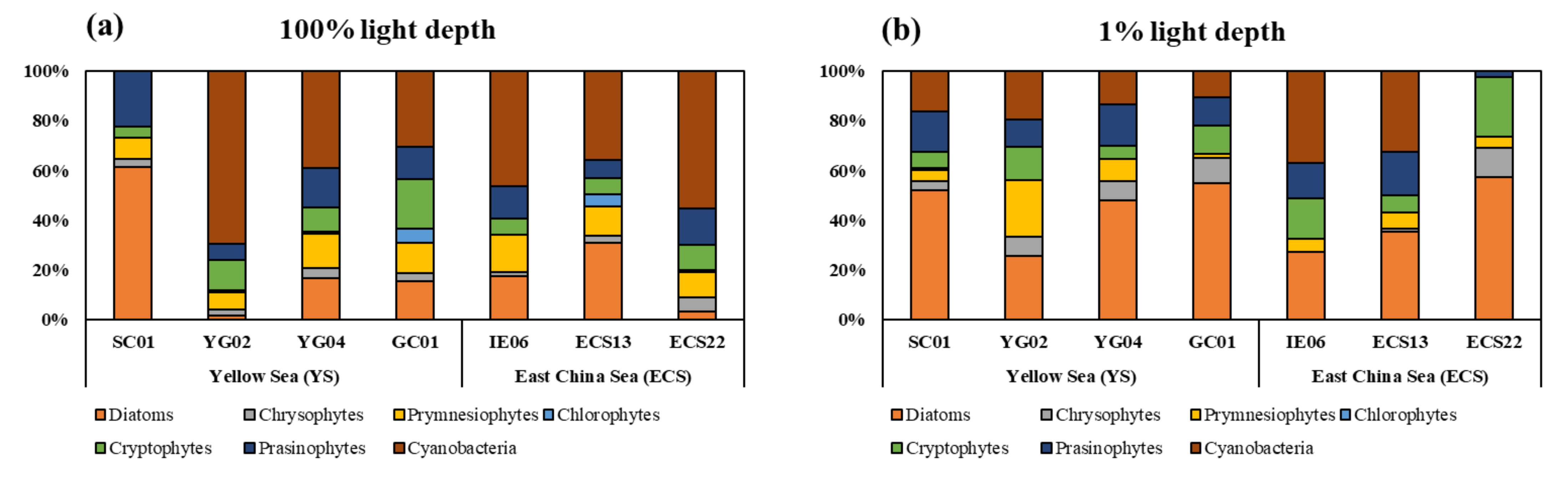
3.3. Phytoplankton Community Structure

The apparent spatial distribution pattern in phytoplankton community composition according to the study regions (i.e., YS and ECS) was not observed during the late summer of 2020 (Figure 4). The major phytoplankton groups were diatoms and cyanobacteria, whereas dinoflagellates were not found in this study (Figure 4). Cyanobacteria made the greatest contribution to the total phytoplankton community at a 100% light depth (range = 30.5–69.5%; mean ± S.D. = 46.1 ± 14.4%) for all the stations except SC01, where diatoms (61.3%) were found to be the dominant class and cyanobacteria were absent (Figure 4a). Diatoms (range = 1.5–31.1%; mean ± S.D. = 14.8 ± 10.8%; except SC01), prymnesiophytes (range = 6.7–14.9%; mean ± S.D. = 11.2 ± 2.9%), cryptophytes (range = 4.3–20.1%; mean ± S.D. = 10.0 ± 5.2%), and prasinophytes (range = 6.4–22.4%; mean ± S.D. = 13.1 ± 5.4%) made medium-level contributions to the total phytoplankton community at a 100% euphotic depth for all the YS and the ECS stations, whereas chrysophytes (range = 2.0–5.7%; mean ± S.D. = 3.4 ± 1.2%) and chlorophytes (range = 0.0–5.6%; mean ± S.D. = 1.9 ± 2.4%) presented low-level contributions (Figure 4a). At a 1% light depth in the study area, the main species that made up the entire phytoplankton community were diatoms (range = 27.2–57.2%; mean ± S.D. = 42.9 ± 13.3%) (Figure 4b). Cyanobacteria (range = 0.0–37.1%; mean ± S.D. = 18.5 ± 12.8%), prasinophytes (range = 2.2–17.4%; mean ± S.D. = 12.7 ± 5.3%), and cryptophytes (range = 5.1–24.1%; mean ± S.D. = 11.9 ± 6.7%) were the ancillary groups in the phytoplankton community composition, whereas the contributions of prymnesiophytes (range = 1.6–22.9%; mean ± S.D. = 7.7 ± 7.0%), chrysophytes (range = 0.0–12.1%; mean ± S.D. = 6.1 ± 4.5%), and chlorophytes (range = 0.0–0.6%; mean ± S.D. = 0.1 ± 0.2%) to the total phytoplankton community were low (Figure 4b).

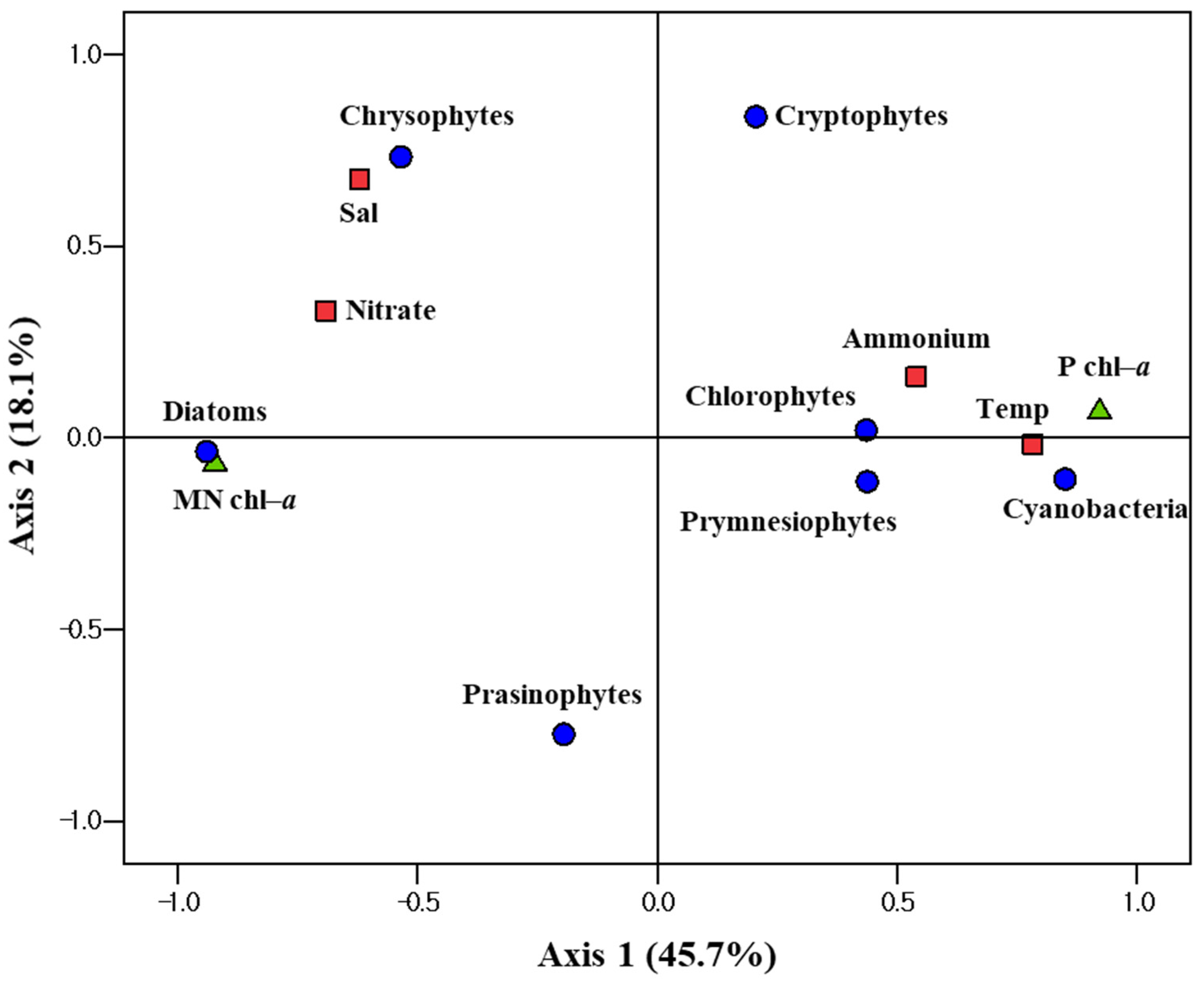
3.4. Relationships between Phytoplankton Groups and Different Environmental Factors

A principal component analysis (PCA; SPSS 12.0) was performed in order to examine the relationships between the phytoplankton groups and different environmental variables (physical factors: temperature and salinity; chemical factors: nitrate and ammonium; biological factors: size-fractionated chlorophyll-a) (Figure 5). The first two ordination axes of the PCA explained 63.8% of the variance in phytoplankton groups in the late summer of 2020 with respect to various environmental factors (Figure 5). The size-fractionated chlorophyll-a data used in the PCA were the ratio of each chlorophyll-a concentration to the total chlorophyll-a concentration in order to match the data for the phytoplankton group calculated from the CHEMTAX analysis. In addition, since the distribution ratio of diatoms had positive correlations with the ratio of micro- (Pearson’s r = 0.56, p < 0.05) and nano-sized (Pearson’s r = 0.67, p < 0.01) chlorophyll-a, the combined values (i.e., ‘MN chl-a’ in Figure 5) of the ratio of micro- and nano-sized chlorophyll-a were used in the PCA to improve the accuracy of the statistical value.

The cyanobacteria, the major dominant phytoplankton group at the surface layer, were positively correlated with the temperature and pico-sized chlorophyll-a. Ammonium was also expected to have a positive effect on the cyanobacteria distributions (Figure 5). In contrast, the distributions of diatoms, the main phytoplankton group at a 1% light depth, were positively correlated with ‘MN chl-a’ and nitrate and negatively correlated with water temperature (Figure 5).

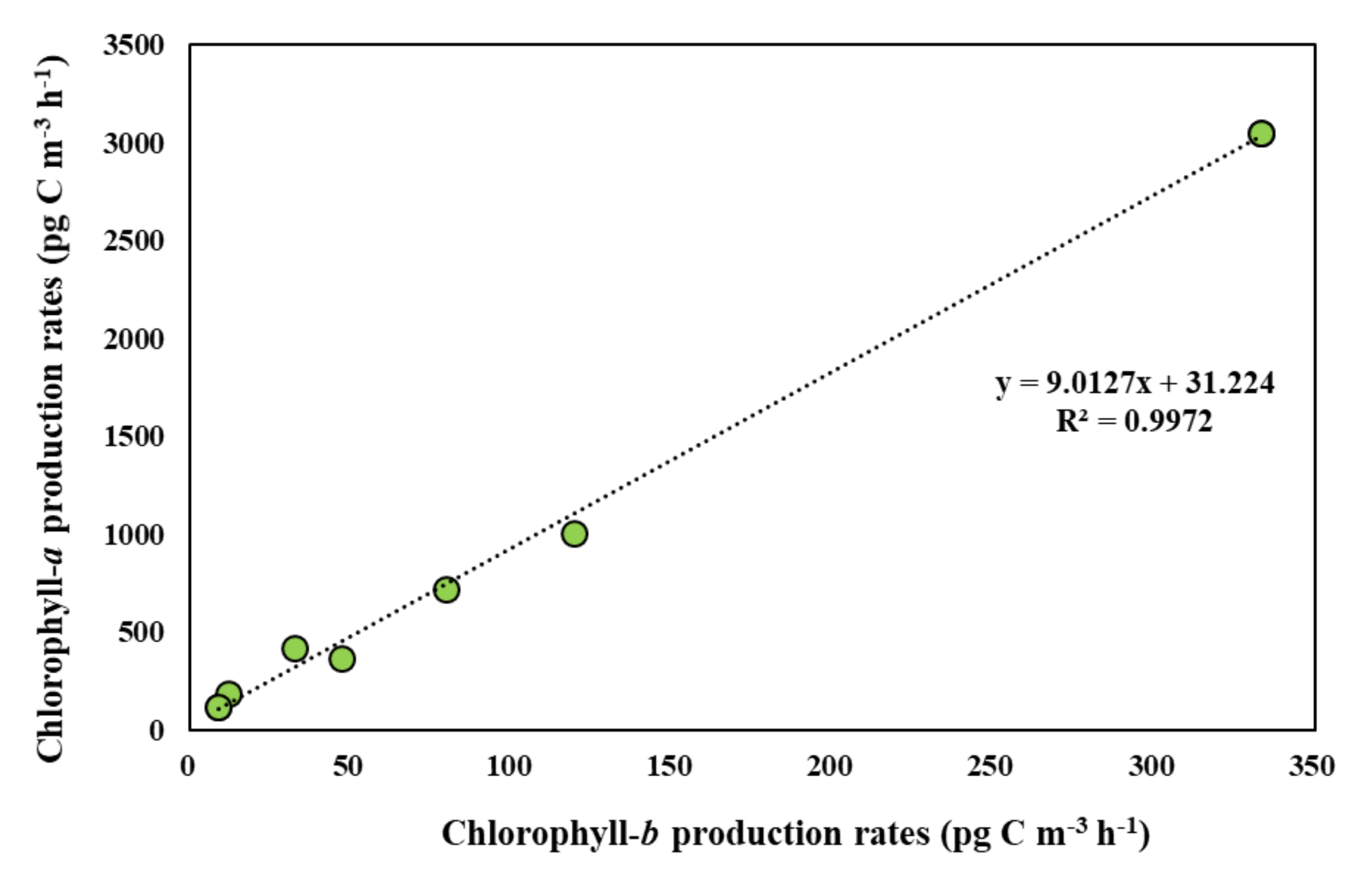
3.5. Photosynthetic Pigment Production Rates

Pigment production rates of the phytoplankton at 100% and 1% light depths in the YS and the ECS are presented in

Table 2. Pigment production rates at 100% and 1% light depths in the study area during late summer of 2020.

* Unit: pg C m−3 h−1			Carotenoid						Chlorophyll		Carotenoid Xanthophyll (Photoprotective Pigment)
	Region	Station	But-fuco	Fuco	Hex-fuco	Neo	Pras	Allo	Chl-b	Chl-a	Diadino	Diato	Viola	Zea
100% light depth	Yellow Sea (YS)	SC01	0.00	48.35	2.34	1.42	1.81	28.86	79.38	719.93	165.75	0.00	6.03	14.62
		YG02	0.00	0.03	0.16	0.00	0.00	7.25	8.71	119.14	0.40	0.53	0.00	52.90
		YG04	0.22	15.56	2.70	4.52	1.44	17.61	332.90	3052.47	52.82	15.70	0.74	336.39
		GC01	0.10	2.03	0.00	0.34	0.03	8.32	32.32	423.36	10.10	4.97	0.00	44.27
	East China Sea (ECS)	IE06	0.00	1.52	0.64	0.27	0.00	1.50	11.54	187.42	1.38	1.78	0.00	27.37
		ECS13	0.16	20.35	1.32	0.16	0.19	3.82	119.26	1008.49	34.34	8.12	0.56	109.18
		ECS22	0.36	1.26	0.00	0.23	0.00	0.53	47.19	367.08	0.00	1.10	0.35	63.84
1% Light depth	Yellow Sea (YS)	SC01	0.00	1.72	0.00	0.02	0.00	0.11	4.16	103.83	0.00	0.00	0.00	0.42
		YG02	0.03	0.00	0.00	0.00	0.00	0.19	3.03	39.46	0.00	0.01	0.00	0.94
		YG04	0.00	0.71	0.00	0.00	0.00	0.16	3.75	24.64	0.00	0.06	0.00	1.52
		GC01	0.00	1.89	1.02	0.00	0.15	0.06	0.00	0.00	0.03	0.00	0.00	0.34
	East China Sea (ECS)	IE06	0.00	1.89	0.02	0.03	0.00	0.00	2.11	6.21	0.00	0.00	0.00	0.38
		ECS13	0.00	5.38	0.12	0.06	0.55	0.20	4.51	107.54	0.06	0.04	0.06	0.22
		ECS22	0.00	3.57	0.63	0.00	0.00	0.65	0.00	0.00	0.12	0.07	0.00	0.00

* But-fuco: 19′-butanoyloxfucoxanthin; Fuco: fucoxanthin; Hex-fuco: 19′-hexanoyloxfucoxanthin; Neo: neoxanthin; Pras: prasinoxanthin; Allo: alloxanthin; Chl-b: chlorophyll-b; Chl-a: chlorophyll-a; Diadino: diadinoxanthin; Diato: diatoxanthin; Viola: violaxanthin; Zea: zeaxanthin.

. Overall, the photosynthetic pigment production rates at the 1% light depth were relatively lower than those of the surface layer in both study regions during this observation period (Table 2). No evident spatial distribution pattern of the pigment production rates was found at the surface layer (Table 2). Most carotenoids (i.e., 19′-butanoyloxyfucoxanthin, 19′-hexanoyloxyfucoxanthin, neoxanthin, and prasinoxanthin) at the 100% light depth had low production rates (<4.52 pg C m⁻³ h⁻¹), whereas fucoxanthin (range = 0.03–48.35 pg C m⁻³ h⁻¹) and alloxanthin (0.53–28.86 pg C m⁻³ h⁻¹) showed slightly higher production rates compared to those of other carotenoids (Table 2). At the surface layer of each station, the production rates of chlorophyll-b (range = 8.71–332.90 pg C m⁻³ h⁻¹) were approximately one tenth those of chlorophyll-a (range = 119.14–3052.47 pg C m⁻³ h⁻¹). In general, the carotenoid xanthophyll (photoprotective pigment) production at the 100% light depth in the YS and ECS was relatively higher in the diadinoxanthin (range = 0.00–165.75 pg C m⁻³ h⁻¹) and zeaxanthin (range = 14.62–336.39 pg C m⁻³ h⁻¹) than in the diatoxanthin (range = 0.00–15.70 pg C m⁻³ h⁻¹) and violaxanthin (range = 0.00–6.03 pg C m⁻³ h⁻¹) (Table 2). All pigment production (carotenoid, chlorophyll, and carotenoid xanthophyll) at the 1% light depth had extremely low values compared to those at the surface layer (Table 2).

4. Discussion

During the study period, no noticeable differences were found in the community composition and pigment production of phytoplankton between the YS and the ECS, but differences in the vertical distribution were observed. Thus, we focused on understanding these vertical distribution characteristics in this study.

The noticeable physical characteristic in this study area was the water column stratification within the euphotic depth (Figure 2). The stratification of the ocean results in diverse environmental conditions, especially in vertical variations in the availability of light and nutrients [36,37]. In other words, sufficient light and poor nutrient conditions can be provided to the upper euphotic zone under stratified conditions, while the opposite conditions appear in deeper zones [29]. The concentrations of nitrate, as one of the most important nutrients for phytoplankton growth [38], were found to be significantly lower (t-test, p < 0.01) at a 100% light depth than at a 1% light depth (Table 1) in this study. The water column during August 2018 [39] was found to be more strongly stratified compared to that observed in our study period. Based on the results of another study, the surface water temperature (mean ± S.D. = 29.1 ± 3.1 °C) for summer 2018 was significantly higher (t-test, p < 0.01) than that found in our study (mean ± S.D. = 24.2 ± 1.6 °C), whereas the temperature at the 1% light depth (mean ± S.D. = 11.2 ± 5.1 °C) during August 2018 was significantly lower (t-test, p < 0.01) than that found in this study (mean ± S.D. = 19.7 ± 4.9 °C). The salinity and ammonium levels were found to be similar between summer 2018 [39] and the timeframe of this study. No difference was found in the nitrate concentration at the surface layer, while the concentration of nitrate at the 1% light depth was found to be two times higher in our observation period (mean ± S.D. = 7.6 ± 3.4 µM) than in summer 2018 (mean ± S.D. = 3.4 ± 1.8 µM) [39]. These different environmental properties of water masses (e.g., temperature, water column stability, nutrient availability, and light intensity) have direct effects on phytoplankton biomass and community composition [29]. Indeed, vertical differences in phytoplankton community structure were observed at each station of this study region (Figure 3 and Figure 4). The main components of the phytoplankton community composition at the 100% light depth were pico-sized phytoplankton (Figure 3a), which were represented by cyanobacteria based on the PCA (Figure 4a and Figure 5), whereas the dominant representative of the phytoplankton group at the 1% light depth (Figure 3b) was large phytoplankton (sum of micro- and nano-sized phytoplankton), which were considered as diatoms on the basis of the PCA (Figure 4b and Figure 5). This vertical distribution characteristic of the phytoplankton community was generally seen in the stratified water mass of the summer season [20,40,41,42,43]. Previous studies conducted in similar regions (YS: [41]; ECS: [40,43]) and periods (i.e., summer seasons) to those used in this study also observed that cyanobacteria dominated at the surface layer (which has a warm temperature and is nutrient-poor), while diatoms were abundant at the deeper layer (with low-temperature and eutrophic conditions). When the water temperature exceeds 20 °C, many cyanobacteria species have relatively high growth rates due to their competitive advantage at warm temperatures, while eukaryotic phytoplankton generally show a stabilization or reduction in their growth rates [44,45,46]. In addition, pico-sized phytoplankton are preferred over larger phytoplankton under nutrient-deficient conditions due to their high nutritional affinity associated with their small cell size [47,48,49], while cyanobacteria appear to have a high preference for ammonium and diatoms preferentially utilize nitrate [38,50,51]. Therefore, the water temperature and nutrient (i.e., nitrate and ammonium) distribution had profound effects on the vertical distributions of phytoplankton communities during our observation period (Figure 5). In addition, the measurement of dissolved organic nitrogen (DON) as one of the important nitrogen sources can be helpful in order to better understand the physiological status of the phytoplankton community within the euphotic zone, although we could not analyze the DON in this study. The DON released by the phytoplankton was an average of 25 to 41% of the uptake nitrogen sources (ammonium or nitrate) [52]. This organic material is assimilated by bacteria and can then be released as ammonium and/or nitrate, and some phytoplankton with cell-surface enzymes can directly take up and utilize DON [52,53]. In [53], the authors observed a relatively higher nitrogen content in DON (mean ± S.D. = 11.9 ± 2.2 µM) than in other types (ammonium: mean ± S.D. = 2.8 ± 4.8 µM; nitrate: mean ± S.D. = 10.5 ± 3.4 µM).

Phytoplankton in natural conditions experience rapid changes in light regime. In order to cope with these dramatic changes in light conditions, phytoplankton can alter their pigment pool, which mostly consists of two functional categories: (1) light harvesting under a low light intensity and (2) photoprotection under a high light intensity [12]. Thus, the pigment production rates were measured in the YS and ECS for the first time to estimate the photophysiological characteristics of the phytoplankton. The pigment production was generally found to be much higher at the surface layer than at the 1% light depth during this study period (Table 2). The main pigment production activity at a 100% light depth during this study period occurred in chlorophyll-b among the accessory pigment (i.e., carotenoid and chlorophyll-b) (Table 2). Most of the chlorophyll-b production at the surface depth was expected to be performed by prasinophytes during our observation period because the key contributor of chlorophyll-b (marker pigment of chlorophytes and prasinophytes) was considered to be prasinophytes based on the low contribution of chlorophytes to the entire phytoplankton community at the 100% light depth (Figure 4a). The authors of [54] reported that pigment–protein complexes and associated pigments in healthy algae undergoing nitrogen-sufficient conditions may have turnover rates close to zero. In addition, low light-acclimated cells generally have a high light-harvesting pigment content and a low amount of photoprotective carotenoids, whereas an inverse relationship is observed for high light-acclimated cells [55,56,57,58]. Thus, the high rate of production of chlorophyll-b by prasinophytes at the surface layer might indicate that they encountered nutrient-deficient and low-light conditions due to their competitive disadvantage compared the major dominant phytoplankton classes, which were mostly cyanobacteria or diatoms. In fact, the concentration of nitrogen sources (nitrate + ammonium) as well as the production rates of diatoxanthin, a photoprotective pigment for prasinophytes, were low at the surface layer of this study region (Table 2). The production rate of chlorophyll-a at the surface layer of each station had a strong positive correlation (R² = 0.9972) with the chlorophyll-b production rate (Figure 6). Based on this relationship, it seems that chlorophyll-a production at the surface depth was also mostly conducted by prasinophytes in order to improve the utilization efficiency of light energy. In other words, prasinophytes might increase the amount of chlorophyll-a and -b they produce in order to obtain energy for photosynthesis from different light wavelengths, thereby avoiding competition with other phytoplankton classes (i.e., cyanobacteria or diatoms). Carotenoids in this study had maximum levels of absorption for blue light (430–470 nm), whereas the maximum absorptions of chlorophyll-a and -b were not only observed for blue light but also for red light (640–660 nm) [59]. The carotenoid xanthophylls play a necessary role in photoprotection [12]. There are three types of the xanthophyll cycle: (1) violaxanthin/antheraxanthin/zeaxanthin (chrysophytes, chlorophytes, and prasinophytes), (2) diadinoxanthin/diatoxanthin (diatoms and prymnesiophytes), and (3) zeaxanthin accumulation (cryptophytes and cyanobacteria) [12]. When the irradiance is high, the first group de-epoxidizes violaxanthin into zeaxanthin via antheraxanthin, the second group production de-epoxidizes x diadinoxanthin into diatoxanthin, and the third group accumulates zeaxanthin without performing de-epoxidation [12]. At the surface layer of our study region, the major production of photoprotective pigment appeared in the zeaxanthin among carotenoid xanthophyll (Table 2). This means that both groups (1) and (3) or one group suffered from photoinhibition under high light exposure. Based on the composition of the phytoplankton community at the surface layer (Figure 4), the cyanobacteria of group (3) were considered to be the main producers of zeaxanthin, a photoprotective pigment, in order to reduce the cell damage caused by strong light intensities during this study. Interestingly, the high production of diadinoxanthin observed at the surface layer of the SC01 station appears to be due to the dominant species in this area, diatoms (Figure 4). When an alga is exposed to low irradiance, a reverse formation of diadinoxanthin from diatoxanthin occurs [60]. Thus, these diatoms are thought to be encountered at times of low light availability, which could result from the self-shading effect [61] of the micro-size phytoplankton (i.e., diatoms) dominating at the surface layer. The low pigment production rates at a 1% light depth might be due to small available amount of light energy reaching this depth.

5. Summary and Conclusions

Our research revealed vertical variations in phytoplankton community composition in the stratified water column during the summer season. The dominant phytoplankton group at the surface layer was mostly cyanobacteria (pico-size), whereas diatoms (micro- and nano-size) had a high level of contribution to the entire phytoplankton community in the deeper layer (1% light depth) in the YS and the ECS during our observation period. Based on the PCA, the major factors found to determine the vertical phytoplankton distribution in this study were water temperature and nitrogen sources (nitrate and ammonium). Cyanobacteria had positive correlations with water temperature and ammonium, while diatoms had a negative correlation with water temperature and a positive correlation with nitrate concentration during our observation period. Recent studies have emphasized the importance of the role of small phytoplankton in a warmer ocean, since the increase in the contribution of small phytoplankton to the entire phytoplankton community could have negative effects on the quantity and quality of food available to upper trophic organisms [6,8,62,63]. Therefore, this comprehensive study on phytoplankton concerning their quantitative and qualitative characteristics as a basic food source as well as their variations in community structure is expected to lead to a better understanding of their potential effects on the entire marine ecosystem in the YS and ECS.

The result found for the pigment production in this study indicated that cyanobacteria encountered excessive irradiance conditions at the surface layer, producing photoprotective pigment (i.e., zeaxanthin) during our observation period. This means that the photosynthetic activity of cyanobacteria, the dominant phytoplankton class at the surface layer in this study, was not optimal. Indeed, [64] reported that a high-light environment under warm temperature conditions has negative effects on the primary productivity of the cyanobacterial community. This research on the pigment production of phytoplankton is expected to provide important clues relating to the various photosynthetic activities of diverse photosynthetic phytoplankton communities under an anticipated warming ocean scenario with a high level of irradiance and warm temperature conditions.

References

1. Elser, J.J.; Elser, M.M.; Carpenter, S.R. Size fraction of algal chlorophyll, carbon fixation and phosphatase activity: Relationships with species-specific size distributions and zooplankton community structure. J. Plankton Res. 1986, 8, 365–383. [Google Scholar] [CrossRef]
2. Iriarte, J.L.; Pizarro, G.; Troncoso, V.A.; Sobarzo, M. Primary production and biomass of size-fractionated phytoplankton off Antofagasta, Chile (23–24°S) during pre-El Niño and El Niño 1997. J. Mar. Syst. 2000, 26, 37–51. [Google Scholar] [CrossRef]
3. Boyce, D.G.; Lewis, M.R.; Worm, B. Global phytoplankton decline over the past century. Nature 2010, 466, 591–596. [Google Scholar] [CrossRef] [PubMed]
4. Anderson, D.M.; Cembella, A.D.; Hallegraeff, G.M. Progress in understanding harmful algal blooms: Paradigm shifts and new technologies for research, monitoring, and management. Annu. Rev. Mar. Sci. 2012, 4, 143–176. [Google Scholar] [CrossRef] [Green Version]
5. Doney, S.C.; Ruckelshaus, M.; Duffy, J.E.; Barry, J.P.; Chan, F.; English, C.A.; Galindo, H.M.; Grebmeier, J.M.; Hollowed, A.B.; Knowlton, N.; et al. Climate change impacts on marine ecosystems. Annu. Rev. Mar. Sci. 2012, 4, 11–37. [Google Scholar] [CrossRef] [PubMed] [Green Version]
6. Morán, X.A.G.; López-Urrutia, Á.; Calvo-díaz, A.; Li, W.K. Increasing importance of small phytoplankton in a warmer ocean. Glob. Chang. Biol. 2010, 16, 1137–1144. [Google Scholar] [CrossRef]
7. Flombaum, P.; Gallegos, J.L.; Gordillo, R.A.; Rincon, J.; Zabala, L.L.; Jiao, N.; Karl, D.M.; Li, W.K.; Lomas, M.W.; Veneziano, D.; et al. Present and future global distributions of the marine Cyanobacteria Prochlorococcus and Synechococcus. Proc. Natl. Acad. Sci. USA 2013, 110, 9824–9829. [Google Scholar] [CrossRef] [PubMed] [Green Version]
8. Kang, J.J.; Jang, H.K.; Lim, J.H.; Lee, D.; Lee, J.H.; Bae, H.; Lee, C.H.; Kang, C.-K.; Lee, S.H. Characteristics of Different Size Phytoplankton for Primary Production and Biochemical Compositions in the Western East/Japan Sea. Front. Microbiol. 2020, 11, 3306. [Google Scholar] [CrossRef]
9. Litchman, E.; Klausmeier, C.A.; Schofield, O.M.; Falkowski, P.G. The role of functional traits and trade-offs in structuring phytoplankton communities: Scaling from cellular to ecosystem level. Ecol. Lett. 2007, 10, 1170–1181. [Google Scholar] [CrossRef]
10. Barton, A.D.; Pershing, A.J.; Litchman, E.; Record, N.R.; Edwards, K.F.; Finkel, Z.V.; Kiørboe, T.; Ward, B.A. The biogeography of marine plankton traits. Ecol. Lett. 2013, 16, 522–534. [Google Scholar] [CrossRef] [PubMed]
11. Finkel, Z.V.; Irwin, A.J.; Schofield, O. Resource limitation alters the 3/4 size scaling of metabolic rates in phytoplankton. Mar. Ecol. Prog. Ser. 2004, 273, 269–279. [Google Scholar] [CrossRef]
12. Roy, S.; Llewellyn, C.A.; Egeland, E.S.; Johnsen, G. (Eds.) Phytoplankton Pigments: Characterization, Chemotaxonomy and Applications in Oceanography; Cambridge University Press: Cambridge, UK, 2011. [Google Scholar]
13. Ha, S.Y.; La, H.S.; Min, J.O.; Chung, K.H.; Kang, S.H.; Shin, K.H. Photoprotective function of mycosporine-like amino acids in a bipolar diatom (Porosira glacialis): Evidence from ultraviolet radiation and stable isotope probing. Diatom Res. 2014, 29, 399–409. [Google Scholar] [CrossRef]
14. Dai, D.J.; Qiao, F.L.; Xia, C.S.; Jung, K.T. A numerical study on dynamic mechanisms of seasonal temperature variability in the Yellow Sea. J. Geophys. Res. 2006, 111, C11S05. [Google Scholar] [CrossRef] [Green Version]
15. Huang, B.Q.; Liu, Y.; Chen, J.X.; Wang, D.Z.; Hong, H.S.; Lv, R.H.; Huang, L.F.; Lin, Y.A.; Wei, H. Temporal and spatial distribution of size-fractioated phytoplankton biomass in East China Sea and Huanghai Sea. Acta Oceanol. Sin. 2006, 28, 156–164, (In Chinese with English Abstract). [Google Scholar]
16. Fu, M.Z.; Wang, Z.L.; Li, Y.; Li, R.; Sun, P.; Wei, X.; Lin, X.; Guo, J. Phytoplankton biomass size structure and its regulation in the southern Yellow Sea (China): Seasonal variability. Cont. Shelf Res. 2009, 29, 2178–2194. [Google Scholar] [CrossRef]
17. Gong, G.C.; Chen, Y.L.L.; Liu, K.K. Chemical hydrography and chlorophyll a distribution in the East China Sea in summer: Implications in nutrient dynamics. Cont. Shelf. Res. 1996, 16, 1561–1590. [Google Scholar] [CrossRef]
18. Liu, X.; Xiao, W.; Landry, M.R.; Chiang, K.-P.; Wang, L.; Huang, B. Responses of phytoplankton communities to environmental variability in the East China Sea. Ecosystems 2016, 19, 832–849. [Google Scholar] [CrossRef]
19. Gardner, W.D.; Chung, S.P.; Richardson, M.J.; Walsh, I.D. The oceanic mixed-layer pump. Deep Sea Res. Part II Top. Stud. Oceanogr. 1995, 42, 757–775. [Google Scholar] [CrossRef]
20. Kwak, J.H.; Lee, S.H.; Hwang, J.; Suh, Y.S.; Park, H.; Chang, K.I.; Kim, K.-R.; Kang, C.-K. Summer primary productivity and phytoplankton community composition driven by different hydrographic structures in the East/Japan Sea and the Western Subarctic Pacific. J. Geophys. Res. Oceans 2014, 119, 4505–4519. [Google Scholar] [CrossRef]
21. Cho, B.C.; Park, M.G.; Shim, J.H.; Choi, D.H. Sea-surface temperature and f-ratio explain large variability in the ratio of bacterial production to primary production in the Yellow Sea. Mar. Ecol. Prog. Ser. 2001, 216, 31–41. [Google Scholar] [CrossRef] [Green Version]
22. Parsons, T.R.; Maita, Y.; Lalli, C.M. A Manual of Chemical and Biological Methods for Seawater Analysis; Pergamon Press: Oxford, UK, 1984. [Google Scholar]
23. Kang, J.J.; Joo, H.; Lee, J.H.; Lee, J.H.; Lee, H.W.; Lee, D.; Kang, C.K.; Yun, M.S.; Lee, S.H. Comparison of biochemical compositions of phytoplankton during spring and fall seasons in the northern East/Japan Sea. Deep Sea Res. Part II Top. Stud. Oceanogr. 2017, 143, 73–81. [Google Scholar] [CrossRef]
24. Lee, S.H.; Joo, H.; Lee, J.H.; Lee, J.H.; Kang, J.J.; Lee, H.W.; Lee, D.; Kang, C.K. Seasonal carbon uptake rates of phytoplankton in the northern East/Japan Sea. Deep Sea Res. Part II Top. Stud. Oceanogr. 2017, 143, 45–53. [Google Scholar] [CrossRef]
25. Kim, B.K.; Joo, H.; Song, H.J.; Yang, E.J.; Lee, S.H.; Hahm, D.; Rhee, T.S.; Lee, S.H. Large seasonal variation in phytoplankton production in the Amundsen Sea. Polar Biol. 2015, 38, 319–331. [Google Scholar] [CrossRef]
26. Hama, T.; Miyazaki, T.; Ogawa, Y.; Iwakuma, T.; Takahashi, M.; Otsuki, A.; Ichimura, S. Measurement of photosynthetic production of a marine phytoplankton population using a stable 13C isotope. Mar. Biol. 1983, 73, 31–36. [Google Scholar] [CrossRef]
27. Ha, S.Y.; Lee, Y.; Kim, M.S.; Kumar, K.S.; Shin, K.H. Seasonal changes in mycosporine-like amino acid production rate with respect to natural phytoplankton species composition. Mar. Drugs 2015, 13, 6740–6758. [Google Scholar] [CrossRef] [Green Version]
28. Jang, S.J.; Park, M.O. Evaluation of grinding effects on the extraction of photosynthetic pigments for HPLC analysis. Sea 2015, 20, 71–77. [Google Scholar] [CrossRef] [Green Version]
29. Kwak, J.H.; Han, E.; Lee, S.H.; Park, H.J.; Kim, K.-R.; Kang, C.-K. A consistent structure of phytoplankton communities across the warm–cold regions of the water mass on a meridional transect in the East/Japan Sea. Deep Sea Res. Part II Top. Stud. Oceanogr. 2017, 143, 36–44. [Google Scholar] [CrossRef]
30. Zapata, M.; Rodríguez, F.; Garrido, J.L. Separation of chlorophylls and carotenoids from marine phytoplankton: A new HPLC method using a reversed phase C8 column and pyridine-containing mobile phases. Mar. Ecol. Prog. Ser. 2000, 195, 29–45. [Google Scholar] [CrossRef] [Green Version]
31. Park, M.O. Composition and distribution of phytoplankton with size fraction results at southwestern East/Japan Sea. Ocean. Sci. J. 2006, 41, 301–313. [Google Scholar] [CrossRef]
32. Mackey, M.D.; Mackey, D.J.; Higgins, H.W.; Wright, S.W. CHEMTAX—A program for estimating class abundances from chemical markers: Application to HPLC measurements of phytoplankton. Mar. Ecol. Prog. Ser. 1996, 144, 256–283. [Google Scholar] [CrossRef] [Green Version]
33. Wright, S.W.; Thomas, D.P.; Marchant, H.J.; Higgins, H.W.; Mackey, M.D.; Mackey, M.D. Analysis of phytoplankton of the Australian sector of the Southern Ocean: Comparisons of microscopy and size frequency data with interpretations of pigment HPLC data using the ‘CHEMTAX’ matrix factorisation program. Mar. Ecol. Prog. Ser. 1996, 144, 285–298. [Google Scholar] [CrossRef]
34. Wright, S.W.; van den Enden, R.L. Phytoplankton community structure and stocks in the Eastern Antarctic marginal ice zone (BROKE survey, January e March 1996) determined by CHEMTAX analysis of HPLC pigment signatures. Deep Sea Res. Part II Top. Stud. Oceanogr. 2000, 47, 2363–2400. [Google Scholar] [CrossRef]
35. Liu, X.; Huang, B.Q.; Huang, Q.; Wang, L.; Ni, X.B.; Tang, Q.S.; Sun, S.; Wei, H.; Liu, S.M.; Li, C.L.; et al. Seasonal phytoplankton response to physical processes in the southern Yellow Sea. J. Sea Res. 2015, 95, 45–55. [Google Scholar] [CrossRef]
36. Dugdale, R.C.; Goering, J.J. Uptake of new and regenerated forms of nitrogen in primary productivity. Limnol. Oceanogr. 1967, 12, 196–206. [Google Scholar] [CrossRef] [Green Version]
37. Venrick, E.L.; McGowan, J.A.; Mantyla, A.W. Deep maxima of photosynthetic chlorophyll in the Pacific Ocean. Fish. Bull. 1973, 71, 41–52. [Google Scholar]
38. Domingues, R.B.; Barbosa, A.B.; Sommer, U.; Galvão, H.M. Ammonium, nitrate and phytoplankton interactions in a freshwater tidal estuarine zone: Potential effects of cultural eutrophication. Aquat. Sci. 2011, 73, 331–343. [Google Scholar] [CrossRef]
39. Jang, H.K.; Youn, S.H.; Joo, H.; Kim, Y.; Kang, J.J.; Lee, D.; Jo, N.; Kim, K.; Kim, M.-J.; Kim, S.; et al. First Concurrent Measurement of Primary Production in the Yellow Sea, the South Sea of Korea, and the East/Japan Sea, 2018. J. Mar. Sci. Eng. 2021, 9, 1237. [Google Scholar] [CrossRef]
40. Furuya, K.; Hayashi, M.; Yabushita, T.; Ishikawa, A. Phytoplankton dynamics in the East China Sea in spring and summer as revealed by HPLC-derived pigment signatures. Deep Sea Res. Part II Top. Stud. Oceanogr. 2003, 50, 367–387. [Google Scholar] [CrossRef]
41. Liu, X.; Huang, B.; Liu, Z.; Wang, L.; Wei, H.; Li, C.; Huang, Q. High-resolution phytoplankton diel variations in the summer stratified central Yellow Sea. J. Oceanogr. 2012, 68, 913–927. [Google Scholar] [CrossRef]
42. Kwak, J.H.; Lee, S.H.; Park, H.J.; Choy, E.J.; Jeong, H.D.; Kim, K.R.; Kang, C.K. Monthly measured primary and new productivities in the Ulleung Basin as a biological” hot spot” in the East/Japan Sea. Biogeosciences 2013, 10, 4405–4417. [Google Scholar] [CrossRef] [Green Version]
43. Kim, Y.; Youn, S.-H.; Oh, H.J.; Kang, J.J.; Lee, J.H.; Lee, D.; Kim, K.; Jang, H.K.; Lee, J.; Lee, S.H. Spatiotemporal Variation in Phytoplankton Community Driven by Environmental Factors in the Northern East China Sea. Water 2020, 12, 2695. [Google Scholar] [CrossRef]
44. Mur, R.; Skulberg, O.; Utkilen, H. Cyanobacteria in the environment. In Toxic Cyanobacteria in Water; Chorus, I., Batram, J., Eds.; E&FN Spon: London, UK, 1999; pp. 15–40. [Google Scholar]
45. Peperzak, L. Climate change and harmful algal blooms in the North Sea. Acta Oecol. 2003, 24, S139–S144. [Google Scholar] [CrossRef]
46. Paerl, H.W.; Huisman, J. Climate change: A catalyst for global expansion of harmful cyanobacterial blooms. Environ. Microbiol. Rep. 2009, 1, 27–37. [Google Scholar] [CrossRef] [PubMed]
47. Smith, R.E.; Kal, J. Size dependence of growth rate, respiratory electron transport system activity and chemical composition in marine diatoms in the laboratory. J. Phycol. 1982, 18, 275–284. [Google Scholar] [CrossRef]
48. Fogg, G.E. Review Lecture-Picoplankton. Proc. R. Soc. Lond. B Biol. Sci. 1986, 228, 1–30. [Google Scholar]
49. Raven, J. The twelfth Tansley Lecture. Small is beautiful: The picophytoplankton. Funct. Ecol. 1998, 12, 503–513. [Google Scholar] [CrossRef]
50. Reed, M.L.; Pinckney, J.L.; Keppler, C.J.; Brock, L.M.; Hogan, S.B.; Greenfield, D.I. The influence of nitrogen and phosphorus on phytoplankton growth and assemblage composition in four coastal, southeastern USA systems. Estuar. Coast. Shelf Sci. 2016, 177, 71–82. [Google Scholar] [CrossRef]
51. Nwankwegu, A.S.; Li, Y.; Huang, Y.; Wei, J.; Norgbey, E.; Ji, D.; Pu, Y.; Nuamah, L.A.; Yang, Z.; Paerl, H.W. Nitrate repletion during spring bloom intensifies phytoplankton iron demand in Yangtze River tributary, China. Environ. Pollut. 2020, 264, 114626. [Google Scholar] [CrossRef]
52. Bronk, D.A.; Glibert, P.M.; Ward, B.B. Nitrogen uptake, dissolved organic nitrogen release, and new production. Science 1994, 265, 1843–1846. [Google Scholar] [CrossRef] [PubMed]
53. Shi, X.; Qi, M.; Tang, H.; Han, X. Spatial and temporal nutrient variations in the Yellow Sea and their effects on Ulva prolifera blooms. Estuar. Coast. Shelf Sci. 2015, 163, 36–43. [Google Scholar] [CrossRef]
54. Goericke, R.; Welschmeyer, N.A. Pigment turnover in the marine diatom Thalassiosira weissflogii. II. The 14CO2-Labeling kinetics of carotenoids. J. Phycol. 1992, 28, 507–517. [Google Scholar] [CrossRef]
55. Johnsen, G.; Prézelin, B.B.; Jovine, R.V.M. Fluorescence excitation spectra and light utilization in two red tide dinoflagellates. Limnol. Oceanogr. 1997, 42, 1166–1177. [Google Scholar] [CrossRef] [Green Version]
56. Stolte, W.; Kraay, G.W.; Noordeloos, A.A.M.; Riegman, R. Genetic and physiological variation in pigment composition of Emiliania huxleyi (Prymnesiophyceae) and the potential use of its pigment rations as a quantitative physiological marker. J. Phycol. 2000, 36, 529–539. [Google Scholar] [CrossRef] [PubMed]
57. Falkowski, P.G.; Chen, Y.-B. Photoacclimation of light harvesting systems in eukaryotic algae. In Light-Harvesting Antennas in Photosynthesis; Green, B.R., Parson, W.W., Eds.; Kluwer Academic: Dordrecht, The Netherlands, 2003; pp. 423–447. [Google Scholar] [CrossRef]
58. Rodríguez, F.; Chauton, M.; Johnsen, G.; Andresen, K.; Olsen, L.M.; Zapata, M. Photoacclimation in phytoplankton: Implications for biomass estimates, pigment functionality and chemotaxonomy. Mar. Biol. 2006, 148, 963–971. [Google Scholar] [CrossRef]
59. Wright, S.W.; Jeffrey, S.W.; Mantoura, R.F.C. (Eds.) Phytoplankton Pigments in Oceanography: Guidelines to Modern Methods; Unesco: Paris, France, 2005. [Google Scholar]
60. Young, A.J.; Frank, H.A. Energy transfer reactions involving carotenoids: Quenching of chlorophyll fluorescence. J. Photochem. Photobiol. B Biol. 1996, 36, 3–15. [Google Scholar] [CrossRef]
61. Agustí, S. Light environment within dense algal populations: Cell size influences on self-shading. J. Plankton Res. 1991, 13, 863–871. [Google Scholar] [CrossRef]
62. Agawin, N.S.; Duarte, C.M.; Agustí, S. Nutrient and temperature control of the contribution of picoplankton to phytoplankton biomass and production. Limnol. Oceanogr. 2000, 45, 591–600. [Google Scholar] [CrossRef]
63. Mousing, E.A.; Ellegaard, M.; Richardson, K. Global patterns in phytoplankton community size structure—Evidence for a direct temperature effect. Mar. Ecol. Prog. Ser. 2014, 497, 25–38. [Google Scholar] [CrossRef] [Green Version]
64. Kehoe, M.; O’Brien, K.R.; Grinham, A.; Burford, M.A. Primary production of lake phytoplankton, dominated by the cyanobacterium Cylindrospermopsis raciborskii, in response to irradiance and temperature. Inland Waters 2015, 5, 93–100. [Google Scholar] [CrossRef]
Figure 1. Overview of the study region with water sampling locations in the YS (4 stations) and the ECS (3 stations) during the late summer (9–13 September) of 2020.
Water 13 03321 g001
Figure 2. Vertical profiles of (a) temperature, (b) salinity, and (c) density at all the experimental stations of the YS and ECS for late summer of 2020.
Water 13 03321 g002
Figure 3. Total (sum of micro-, nano-, and pico-size chlorophyll-a) and size-fractionated chlorophyll-a concentrations at (a) 100% and (b) 1% light depths in the YS and the ECS during the study period.
Water 13 03321 g003
Figure 4. Relative contributions of different phytoplankton groups to total phytoplankton biomass at (a) 100% and (b) 1% light depths in the YS and ECS during the study period.
Water 13 03321 g004
Figure 5. Principle component analysis (PCA) ordination plots of axes 1 and 2 showing the phytoplankton community structure in relation to physical (temperature and salinity), chemical (nitrate and ammonium), and biological (size-fractionated chlorophyll-a) environmental variables in the YS and ECS during late summer of 2020. Temp: water temperature; Sal: salinity; MN chl-a: sum of the ratio of micro- and nano-sized chlorophyll-a concentration to total chlorophyll-a concentration; P chl-a: ratio of pico-sized chlorophyll-a concentration to total chlorophyll-a concentration.
Water 13 03321 g005
Figure 6. The correlation between the production rates of chlorophyll-b and chlorophyll-a at the surface layer of the YS and ECS.
Water 13 03321 g006