Time-Delayed Bioreactor Model of Phenol and Cresol Mixture Degradation with Interaction Kinetics

Abstract

This paper is devoted to a mathematical model for phenol and p-cresol mixture degradation in a continuously stirred bioreactor. The biomass specific growth rate is presented as sum kinetics with interaction parameters (SKIP). A discrete time delay is introduced and incorporated into the biomass growth response. These two aspects—the mutual influence of the two substrates and the natural biological time delay in the biomass growth rate—are new in the scientific literature concerning bioreactor (chemostat) models. The equilibrium points of the model are determined and their local asymptotic stability as well as the occurrence of local Hopf bifurcations are studied in dependence on the delay parameter. The existence and uniqueness of positive solutions are established, and the global stabilizability of the model dynamics is proved for certain values of the delay. Numerical simulations illustrate the global behavior of the model solutions as well as the transient oscillations as a result of the Hopf bifurcation. The performed theoretical analysis and computer simulations can be successfully used to better understand the biodegradation dynamics of the chemical compounds in the bioreactor and to predict and control the system behavior in real life conditions.

1. Introduction

Wastewater treatment is essential for public health and environmental protection. This is a specific process for removing various contaminants from wastewater. The idea is to safely release treated water into the environment or reuse it. In this regard, practical research related to the hydraulic efficiency of green–blue flood control scenarios for vegetated rivers is currently being expanded [1]. The extent to which wastewater needs to be treated is determined by government water management standards and the specifics of the environment [2]. The treatment process takes place in wastewater treatment plants or a bioreactor. The main methods used for wastewater treatment are mechanical, biological, and chemical. Biological wastewater treatment is performed under aerobic or anaerobic conditions for biomass growth depending on the specific microorganisms used as well as on the nature and concentrations of the contained pollutants [3,4]. The choice of a particular method depends on the type of polluted water and the nature and concentrations of the pollutants.

The main pollutants of industrial and domestic wastewater are plant nutrients, individual or mixtures of synthetic organic chemicals, inorganic chemicals including heavy metals, pathogenic organisms, oil, sediments, radioactive substances, etc. [5].

Some of the most toxic and common mixtures of synthetic organic chemicals are phenol and its derivatives including resorcinol, hydroquinone, 3-nitrophenol, 2,6-dinitrophenol, 3-chlorophenol, p-cresol (4-methylphenol), benzene, etc. Numerous scientific studies and practical applications have proven the potential of several microorganisms to biodegrade mixtures of phenol and its derivatives to environmentally friendly substances [6,7,8]. It has been found that very good results in the biodegradation of phenolic compounds are achieved by the strains Arthrobacter, Aspergillus awamori, Burkholderia, Candida tropicalis, Pseudomonas, Rhodococcus, Trametes hirsute, Trichosporon cutaneum, just to mention a few [9,10,11,12].

Generally speaking, the kinetics describing microbial growth and biodegradation of phenolic components (substrates) are of great importance for studying the peculiarities of the wastewater treatment process [13]. Kinetic models are developed on the basis of expert knowledge and laboratory research with specific strains and particular water pollutants. The kinetic models provide opportunities to study various characteristics of the wastewater treatment process and support the successful and effective achievement of the prescribed environmental criteria [14].

Specific microorganisms’ growth rates in a substrate mixture of two or more phenolic components are known as sum kinetic models (without interaction); multiplication kinetic models; sum kinetic models which incorporate purely competitive substrate kinetics; sum kinetics with interaction parameters (SKIP); elimination capacity-sum kinetics with interaction parameter (EC-SKIP); self-inhibition EC-SKIP (SIEC-SKIP), etc. [15,16,17,18,19,20].

The SKIP models are a successful extension of the sum kinetics models, because they take into account the mutual influence of the components in the substrate mixture [21,22]. The SKIP models demonstrate excellent prediction of the biodegradation with different microbial strains of the mixture of phenol and its derivatives: benzene, toluene, and phenol biodegradation by Pseudomonas putida F1 [23]; ethylbenzene and styrene by R. pyridinovorans PYJ-1 [22]; phenol and p-cresol mixture degradation by Aspergillus awamori strain [24], etc.

In [25], a mathematical model was proposed for phenol and p-cresol mixture degradation in a continuously stirred tank bioreactor. The model was presented by a system of three nonlinear ordinary differential equations as follows

$$\begin{array}{ccc}\hfill {\displaystyle \frac{dX\left(t\right)}{dt}}& =& \left(\mu (S_{ph},S_{cr})-D\right)X\left(t\right)\hfill \\ \hfill {\displaystyle \frac{d{S}_{ph}\left(t\right)}{dt}}& =& -k_{ph}\mu (S_{ph},S_{cr})X\left(t\right)+D(S_{ph}^0-S_{ph}\left(t\right))\hfill \\ \hfill {\displaystyle \frac{d{S}_{cr}\left(t\right)}{dt}}& =& -k_{cr}\mu (S_{ph},S_{cr})X\left(t\right)+D(S_{cr}^0-S_{cr}\left(t\right)),\hfill \end{array}$$

(1)

where $\mu (S_{ph},S_{cr})$ is the biomass specific growth rate, described by the SKIP (sum kinetics with interaction parameters) model in the form

$$\mu (S_{ph},S_{cr})={\displaystyle \frac{{\mu }_{max\left(ph\right)}{S}_{ph}}{k_{s\left(ph\right)}+S_{ph}+\frac{S_{ph}^2}{k_{i\left(ph\right)}}+I_{cr/ph}{S}_{cr}}}+{\displaystyle \frac{{\mu }_{max\left(cr\right)}{S}_{cr}}{k_{s\left(cr\right)}+S_{cr}+\frac{S_{cr}^2}{k_{i\left(cr\right)}}+I_{ph/cr}{S}_{ph}}}.$$

(2)

In the analytic expression of $\mu (·)$, the interaction parameters $I_{cr/ph}$ and $I_{ph/cr}$ indicate the degree to which the substrates p-cresol and phenol affect the biodegradation of phenol and p-cresol, respectively. Two inhibition parameters, $k_{i\left(ph\right)}$ and $k_{i\left(cr\right)}$, are also included in the biomass specific growth rate $\mu (·)$.

The state variables X, $S_{ph}$, $S_{cr}$, and the model parameters are described in Table 1. The numerical values in the last column were validated by laboratory experiments using the Aspergillus awamori strain and given in [24].

Table 1. Model variables and parameters.

	Definitions	Values
X	biomass concentration [g/dm${}^3]$	–
$S_{ph}$	phenol concentration [g/dm${}^3]$	–
$S_{cr}$	p-cresol concentration [g/dm${}^3]$	–
D	dilution rate $\left[h^{-1}\right]$	–
$S_{ph}^0$	influent phenol concentration [g/dm${}^3]$	0.7
$S_{cr}^0$	influent p-cresol concentration [g/dm${}^3]$	0.3
$k_{ph}$	metabolic coefficient $[S_{ph}/X]$	11.7
$k_{cr}$	metabolic coefficient $[S_{cr}/X]$	5.8
$k_{i\left(ph\right)}$	inhibition constant for cell growth on phenol [g/dm${}^3]$	0.61
$k_{i\left(cr\right)}$	inhibition constant for cell growth on cresol [g/dm${}^3]$	0.45
$I_{ph/cr}$	interaction coefficient indicating the degree to which phenol affects the p-cresol biodegradation	0.3
$I_{cr/ph}$	interaction coefficient indicating the degree to which p-cresol affects the phenol biodegradation	8.6
${\mu }_{max\left(ph\right)}$	maximum specific growth rate on phenol as a single substrate $\left[h^{-1}\right]$	0.23
${\mu }_{max\left(cr\right)}$	maximum specific growth rate on p-cresol as a single substrate $\left[h^{-1}\right]$	0.17
$k_{s\left(ph\right)}$	saturation constant for cell growth on phenol [g/dm${}^3]$	0.11
$k_{s\left(cr\right)}$	saturation constant for cell growth on p-cresol [g/dm${}^3]$	0.35

In this paper, we modify model (1) by introducing a discrete time delay incorporated into the biomass growth response

$$\begin{array}{ccc}\hfill {\displaystyle \frac{dX\left(t\right)}{dt}}& =& e^{-D\tau }\mu (S_{ph}(t-\tau ),S_{cr}(t-\tau ))X(t-\tau )-DX\left(t\right)\hfill \end{array}$$

(3)

$$\begin{array}{ccc}\hfill {\displaystyle \frac{d{S}_{ph}\left(t\right)}{dt}}& =& -k_{ph}\mu (S_{ph}\left(t\right),S_{cr}\left(t\right))X\left(t\right)+D(S_{ph}^0-S_{ph}\left(t\right))\hfill \end{array}$$

(4)

$$\begin{array}{ccc}\hfill {\displaystyle \frac{d{S}_{cr}\left(t\right)}{dt}}& =& -k_{cr}\mu (S_{ph}\left(t\right),S_{cr}\left(t\right))X\left(t\right)+D(S_{cr}^0-S_{cr}\left(t\right)).\hfill \end{array}$$

(5)

The constant $\tau \ge 0$ stands for the time delay in the conversion of the consumed substrate into viable biomass. The term ${\displaystyle e^{-D\tau }X(t-\tau )}$ represents the biomass of microorganisms that consumes nutrients at time $t-\tau$ and survives in the bioreactor for $\tau$ units of time, necessary to complete the conversion of substrate into viable biomass [26,27].

Bioreactor (chemostat) competition models involving time delay, recently, have been widely discussed and investigated in the literature. According to [28], the conversion process of nutrients to biomass always requires a fixed length of time and thus the corresponding chemostat model should be described by a system of differential equations with discrete delays. To our knowledge, the first attempt to introduce a discrete time delay was in [29], where a linear bioreactor model was discussed. Other early models in this regard can be found in [30], where the effects of time delay and growth rate inhibition in the bacterial treatment of wastewater were discussed, as well as in [31], where the appearance of a time delay was motivated by the existence of a lag phase in the growth response of microorganisms in the medium. A basic and well known chemostat model incorporating a time delay was proposed and studied in [32]. This model contained three nonlinear ordinary differential equations, describing competition of two species on a single nutrient, and established the validity of the Competitive Exclusion Principle (CEP). CEP means that the species with the lowest break-even concentration can survive in the chemostat, and it drives other species to extinction. Two-species competition was also considered in [33], where CEP was proved as well. On the other hand, introducing a time delay explicitly into the model equations can help to explain the transient oscillation behavior of the bioreactor dynamics often observed in practical experiments. Detailed investigations in this direction can be found in [34] on a ‘single biomass/single substrate’ model.

Recently, various mathematical delayed models involving different numbers of species growing on one or more substrates and involving different kinds of specific growth rates (monotone, such as the Monod law, or nonmonotone, such as the Haldane law, etc.) have been discussed, see [26,27,35] and the references therein. The latter papers consider competition of n species of microorganisms on a single substrate. In [26], sufficient conditions are presented which enhance the CEP and thus the global asymptotic stability of the model solutions. This was calculated for general nonmonotone response (specific growth rate) functions. The same time delayed model was modified in [27] by introducing specific species death rates, different from the dilution rate in the chemostat. Under certain conditions, it was shown that the single species survival equilibrium is globally asymptotically stable. It was demonstrated numerically that the differential removal rates can lead to damped oscillation in the solutions. Similar results were established for the same model in [35]. There, the competitive exclusion was established by applying the method of Liapunov functionals under some technical assumptions on the biomass response functions.

In this paper, we perform mathematical analysis of the time delayed model (3)–(5). In Section 2, we find the equilibrium points of the model and investigate their local asymptotic stability and occurrence of Hopf bifurcations with respect to the delay $\tau$. The basic properties of the model solutions as well as the global stabilizability of the model dynamics are presented in Section 3. Section 4 includes numerical examples, supporting the theoretical results. Concluding remarks are presented in Section 5.

2. Equilibrium Points, Local Stability, and Bifurcations

In the mathematical analysis of the model (3)–(5), we assume that the influent concentrations $S_{ph}^0$ and $S_{cr}^0$ are constant and consider the dilution rate D and the delay $\tau$ as varying parameters.

The equilibrium points of (3)–(5) are obtained as solutions of the following system of transcendental equations

$$\begin{array}{ccc}& & e^{-D\tau }\mu (S_{ph},S_{cr})X-DX=0\hfill \end{array}$$

(6)

$$\begin{array}{ccc}& & -k_{ph}\mu (S_{ph},S_{cr})X+D(S_{ph}^0-S_{ph})=0\hfill \end{array}$$

(7)

$$\begin{array}{ccc}& & -k_{cr}\mu (S_{ph},S_{cr})X+D(S_{cr}^0-S_{cr})=0.\hfill \end{array}$$

(8)

Obviously, $E_0=(0,S_{ph}^0,S_{cr}^0)$ (with $X=0$) is an equilibrium point of the model for all $D>0$ and $\tau \ge 0$ and is called the boundary or washout equilibrium.

In what follows, we look for solutions of (6)–(8) such that $X>0$.

Similar to [25], multiplying Equation (7) by $-k_{cr}$, Equation (8) by $k_{ph}$, and summing them together leads to

$$-k_{cr}(S_{ph}^0-S_{ph})+k_{ph}(S_{cr}^0-S_{cr})=0.$$

(9)

Denoting

$$K={\displaystyle \frac{k_{ph}}{k_{cr}}},S^0=S_{ph}^0-K{S}_{cr}^0,$$

(10)

we obtain

$$S_{ph}=S_{ph}^0-{\displaystyle \frac{k_{ph}}{k_{cr}}}\left(S_{cr}^0-S_{cr}\right)=(S_{ph}^0-{\displaystyle \frac{k_{ph}}{k_{cr}}}{S}_{cr}^0)+{\displaystyle \frac{k_{ph}}{k_{cr}}}{S}_{cr}=S^0+K{S}_{cr}.$$

(11)

The latter expression is biologically relevant if and only if $S^0\ge 0$. Using the numerical values in the last column of Table 1, it follows that this is satisfied: $S^0\approx 0.09483$.

Now, we substitute $S_{ph}$ from (11) into the expression of $\mu (S_{ph},S_{cr})$ and obtain the specific growth rate $\mu (·)$ as a function of $S_{cr}$ only. Denote for simplicity

$${\mu }_{cr}\left(S_{cr}\right)=\mu (S^0+K{S}_{cr},S_{cr}),$$

(12)

or explicitly

$$\begin{array}{c}{\mu }_{cr}\left(S_{cr}\right)={\displaystyle \frac{{\mu }_{max\left(ph\right)}\left(S^0+K{S}_{cr}\right)}{k_{s\left(ph\right)}+S^0+K{S}_{cr}+\frac{1}{k_{i\left(ph\right)}}{(S^0+K{S}_{cr})}^2+I_{cr/ph}{S}_{cr}}}\hfill \\ +{\displaystyle \frac{{\mu }_{max\left(cr\right)}{S}_{cr}}{k_{s\left(cr\right)}+S_{cr}+\frac{1}{k_{i\left(cr\right)}}{S}_{cr}^2+I_{ph/cr}(S^0+K{S}_{cr})}}.\hfill \end{array}$$

(13)

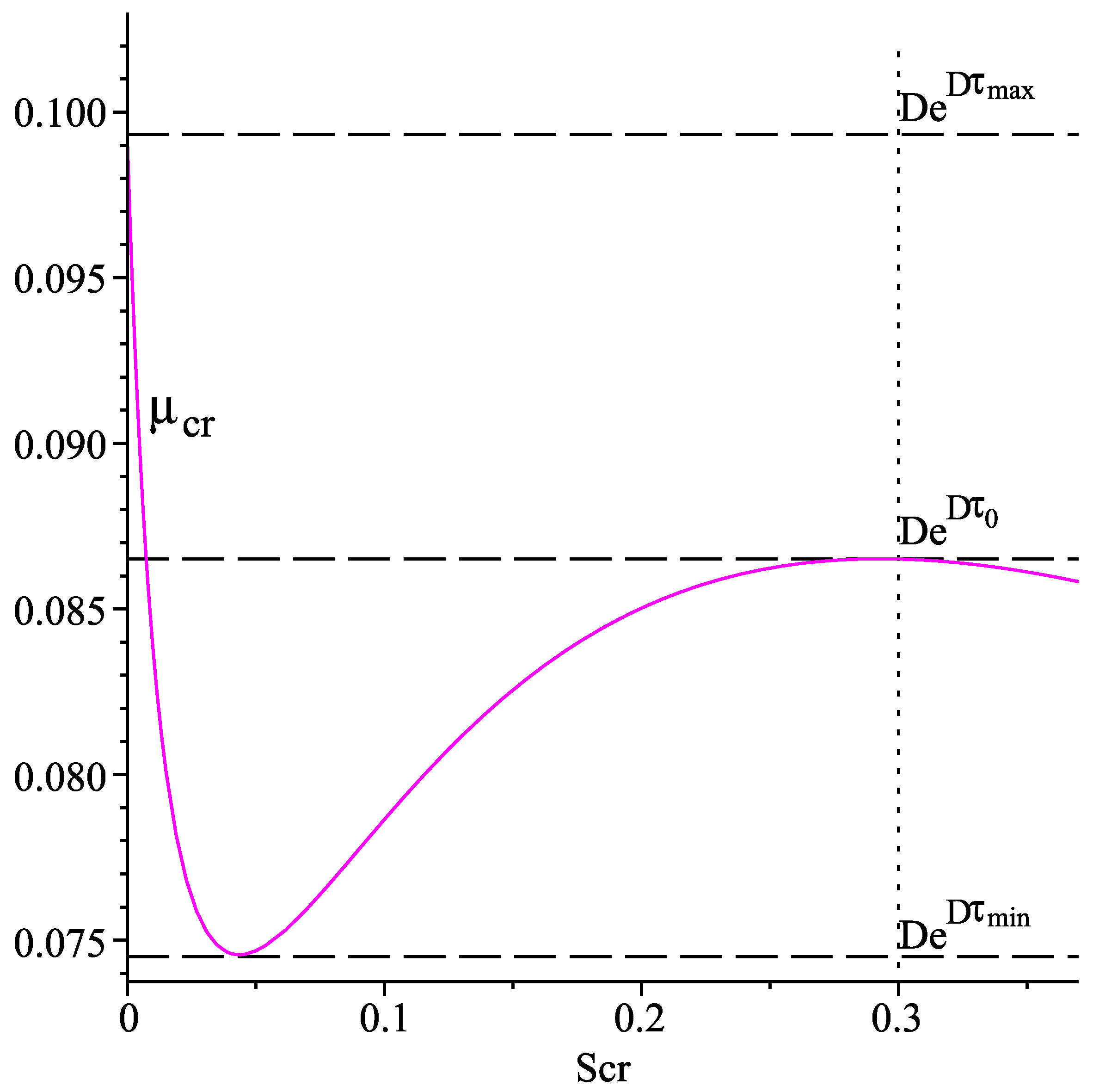
Figure 1 shows the graph of the function ${\mu }_{cr}\left(S_{cr}\right)$ for $S_{cr}\ge 0$, using the numerical values in the last column of Table 1.

Figure 1. Graph of the function ${\mu }_{cr}\left(S_{cr}\right)$ for $S_{cr}\ge 0$. The vertical dot line passes through $S_{cr}^0$.

From Equation (6), we learn that the steady state component with respect to $S_{cr}$ is the solution of the equation

$${\mu }_{cr}\left(S_{cr}\right)=D{e}^{D\tau }.$$

(14)

If there exists a root $S_{cr}^{*}$ of the latter, such that $0<S_{cr}^{*}<S_{cr}^0$, then the equilibrium components with respect to X and $S_{ph}$ are determined by the formulae

$$S_{ph}^{*}=S^0+K{S}_{cr}^{*},X^{*}={\displaystyle \frac{S_{cr}^0-S_{cr}^{*}}{k_{cr}{e}^{D\tau }}}={\displaystyle \frac{S_{ph}^0-S_{ph}^{*}}{k_{ph}{e}^{D\tau }}}$$

(15)

Denote $E^{*}=(X^{*},S_{ph}^{*},S_{cr}^{*})$. Obviously, all components of $E^{*}$ depend on the control parameter D and on the delay $\tau$.

The graph of ${\mu }_{cr}\left(S_{cr}\right)$ suggests the following properties of the latter, which are used in the further investigations.

Properties of ${\mu }_{cr}\left(S_{cr}\right)$

(P1)${\mu }_{cr}\left(S_{cr}\right)>0$ for all $S_{cr}\ge 0$, and ${\mu }_{cr}\left(0\right)=\frac{{\mu }_{max\left(ph\right)}{S}^0}{k_{s\left(ph\right)}+S^0+\frac{{S^0}^2}{k_{i\left(ph\right)}}}>0$.

(P2) There exists a point $S_{cr}^{min}\in (0,S_{cr}^0)$ such that $\frac{d}{d{S}_{cr}}{\mu }_{cr}\left(S_{cr}\right)<0$ if $S_{cr}\in [0,S_{cr}^{min})\cup (S_{cr}^0,+\infty )$, and ${\displaystyle \frac{d}{d{S}_{cr}}}{\mu }_{cr}\left(S_{cr}\right)>0$ if $S_{cr}\in (S_{cr}^{min},S_{cr}^0)$.

(P3) The following inequalities hold true: ${\mu }_{cr}\left(S_{cr}^{min}\right)<{\mu }_{cr}\left(S_{cr}^0\right)<{\mu }_{cr}\left(0\right)$.

For any $D>0$ define

$$\begin{array}{c}{\tau }_{min}={\tau }_{min}\left(D\right)={\displaystyle \frac{1}{D}}ln{\displaystyle \frac{{\mu }_{cr}\left(S_{cr}^{min}\right)}{D}},\hfill \\ {\tau }_{max}={\tau }_{max}\left(D\right)={\displaystyle \frac{1}{D}}ln{\displaystyle \frac{{\mu }_{cr}\left(0\right)}{D}},\hfill \\ {\tau }_0={\tau }_0\left(D\right)={\displaystyle \frac{1}{D}}ln{\displaystyle \frac{{\mu }_{cr}\left(S_{cr}^0\right)}{D}}.\hfill \end{array}$$

(16)

Obviously, $\tau =\tau \left(D\right)$ is a decreasing function of $D>0$. Moreover, for any $D>0$, the following inequalities are fulfilled:

$${\tau }_{min}<{\tau }_0<{\tau }_{max}.$$

Based on the above considerations we draw the following conclusions:

• If $\tau \in ({\tau }_{min},{\tau }_0)$, then there exist two positive roots $S_{cr}^{\left(1\right)}=S_{cr}^{\left(1\right)}\left(\tau \right)$, $S_{cr}^{\left(2\right)}=S_{cr}^{\left(2\right)}\left(\tau \right)$ of Equation (14) such that $S_{cr}^{\left(1\right)}<S_{cr}^{\left(2\right)}<S_{cr}^0$, and $\frac{d}{d\tau }{S}_{cr}^{\left(1\right)}\left(\tau \right)<0$, $\frac{d}{d\tau }{S}_{cr}^{\left(2\right)}\left(\tau \right)>0$.
• If $\tau \in ({\tau }_0,{\tau }_{max}]$, then there is only one positive root $S_{cr}^{\left(1\right)}\left(\tau \right)<S_{cr}^0$ of Equation (14) such that $\frac{d}{d\tau }{S}_{cr}^{\left(1\right)}\left(\tau \right)<0$ and $S_{cr}^{\left(1\right)}\left({\tau }_{max}\right)=0$.

Therefore, the model (3)–(5) possesses up to two interior (with positive components) equilibrium points depending on the values of $\tau$ and D. Denote them by

$$\begin{array}{ccc}\hfill E_1=E_1(D;\tau )& =& \left(X^{\left(1\right)},S_{ph}^{\left(1\right)},S_{cr}^{\left(1\right)}\right),\tau \in \left({\tau }_{min},{\tau }_{max}\right);\hfill \\ \hfill E_2=E_2(D;\tau )& =& \left(X^{\left(2\right)},S_{ph}^{\left(2\right)},S_{cr}^{\left(2\right)}\right),\tau \in \left({\tau }_{min},{\tau }_0\right),with{S}_{cr}^{\left(2\right)}>S_{cr}^{\left(1\right)},\hfill \end{array}$$

where $X^{\left(i\right)}$ and $S_{ph}^{\left(i\right)}$, $i=1,2$, are determined according to (15) after replacing the ${}^{*}$ with ${}^{\left(1\right)}$ and ${}^{\left(2\right)}$, respectively.

In what follows, we study the local asymptotic stability of the model equilibrium points. Here, we use the linearization technique for differential equations with a discrete time delay (see [36]).

The characteristic polynomial corresponding to the Jacobian matrix J of (3)–(5) is defined by $det(J-\lambda I_3)$, where $\lambda$ is any complex number, and $I_3$ is the $(3\times 3)$–identity matrix:

$$\begin{array}{c}\hfill {\displaystyle det(J-\lambda I_3)=}\\ & \left|\begin{array}{ccc}{e}^{-(\lambda +D)\tau }\mu (S_{ph},S_{cr})-D-\lambda \hfill & e^{-(\lambda +D)\tau }\frac{\partial \mu }{\partial S_{ph}}X\hfill & e^{-(\lambda +D)\tau }\frac{\partial \mu }{\partial S_{cr}}X\hfill \\ -k_{ph}\mu (S_{ph},S_{cr})\hfill & -k_{ph}\frac{\partial \mu }{\partial S_{ph}}X-D-\lambda \hfill & -k_{ph}\frac{\partial \mu }{\partial S_{cr}}X\hfill \\ -k_{cr}\mu (S_{ph},S_{cr})\hfill & -k_{cr}\frac{\partial \mu }{\partial S_{ph}}X\hfill & -k_{cr}\frac{\partial \mu }{\partial S_{cr}}X-D-\lambda \hfill \end{array}\right|.\hfill \end{array}$$

The following presentation holds true

$$\begin{array}{c}det(J-\lambda I_3)=\hfill \\ {(D+\lambda )}^2\left[\left(D+\lambda +X\left(k_{ph}\frac{\partial \mu }{\partial S_{ph}}+k_{cr}\frac{\partial \mu }{\partial S_{cr}}\right)\right)-e^{-(\lambda +D)\tau }\mu (S_{ph},S_{cr})\right].\hfill \end{array}$$

(17)

Obviously, ${\lambda }_{1,2}=-D<0$ are always solutions of $det(J\left(E_i\right)-\lambda I_3)=0$, i.e., eigenvalues of the Jacobian matrix $J\left(E_i\right)$ evaluated at the equilibrium point $E_i$, $i=0,1,2$. The third eigenvalue ${\lambda }_3$ of (17) is the root of the equation

$$\lambda +D+X\left(k_{ph}\frac{\partial \mu }{\partial S_{ph}}+k_{cr}\frac{\partial \mu }{\partial S_{cr}}\right)-e^{-D\tau }\mu (S_{ph},S_{cr})e^{-\lambda \tau }=0,$$

(18)

the latter being evaluated at the components of $E_i$, $i=0,1,2$.

Straightforward calculations show that

$$\begin{array}{c}{\left.\left(k_{ph}{\displaystyle \frac{\partial \mu }{\partial S_{ph}}}+k_{cr}{\displaystyle \frac{\partial \mu }{\partial S_{cr}}}\right)\right|}_{S_{ph}=S^0+K{S}_{cr}}=k_{cr}{\displaystyle \frac{d}{d{S}_{cr}}}{\mu }_{cr}\left(S_{cr}\right)\hfill \\ ={\displaystyle \frac{{\mu }_{max\left(ph\right)}}{A^2}}\left[k_{ph}\left(k_{s\left(ph\right)}-{\displaystyle \frac{{(S^0+K{S}_{cr})}^2}{k_{i\left(ph\right)}}}\right)-k_{cr}{I}_{cr/ph}{S}^0\right]\hfill \\ +{\displaystyle \frac{{\mu }_{max\left(cr\right)}{k}_{cr}}{B^2}}\left[k_{s\left(cr\right)}-{\displaystyle \frac{S_{cr}^2}{k_{i\left(cr\right)}}}+I_{cr/ph}{S}^0\right],\hfill \end{array}$$

where

$$\begin{array}{ccc}\hfill A& =& k_{s\left(ph\right)}+S^0+K{S}_{cr}+\frac{1}{k_{i\left(ph\right)}}{(S^0+K{S}_{cr})}^2+I_{cr/ph}{S}_{cr},\hfill \\ \hfill B& =& k_{s\left(cr\right)}+S_{cr}+\frac{S_{cr}^2}{k_{i\left(cr\right)}}+I_{ph/cr}(S^0+K{S}_{cr}).\hfill \end{array}$$

Therefore, the characteristic Equation (18) can be rewritten in the form

$$\lambda +D+X{k}_{cr}{\mu }_{cr}^{\prime }\left(S_{cr}\right)-e^{-D\tau }{\mu }_{cr}\left(S_{cr}\right)e^{-\lambda \tau }=0,$$

(19)

where ${\mu }_{cr}^{\prime }\left(S_{cr}\right)$ means ${\displaystyle \frac{d}{d{S}_{cr}}}{\mu }_{cr}\left(S_{cr}\right)$.

In the next subsections, we study the local asymptotic stability and existence of Hopf bifurcations of the equilibrium points with respect to the delay $\tau >0$.

2.1. The Interior Equilibrium $E_2$

The interior equilibrium $E_2=E_2\left(\tau \right)=(X^{\left(2\right)},S_{ph}^{\left(2\right)},S_{cr}^{\left(2\right)})$ exists for $\tau \in \left({\tau }_{min},{\tau }_0\right)$ and

$$\begin{array}{c}{S}_{cr}^{\left(2\right)}\mathrm{is}\mathrm{a}\mathrm{solution}\mathrm{of}{\mu }_{cr}\left(S_{cr}\right)=D{e}^{D\tau },\hfill \\ S_{ph}^{\left(2\right)}=S^0+K{S}_{cr}^{\left(2\right)},X^{\left(2\right)}={\displaystyle \frac{S_{cr}^0-S_{cr}^{\left(2\right)}}{k_{cr}{e}^{D\tau }}}={\displaystyle \frac{S_{ph}^0-S_{ph}^{\left(2\right)}}{k_{ph}{e}^{D\tau }}}.\hfill \end{array}$$

Proposition 1.

For the model (3)–(5), the equilibrium point $E_2$ is locally asymptotically stable for all $\tau \in ({\tau }_{min},{\tau }_0)$.

Proof. 

The characteristic Equation (19) evaluated at $E_2=(X^{\left(2\right)},S_{ph}^{\left(2\right)},S_{cr}^{\left(2\right)})$ is

$$\lambda +D+X^{\left(2\right)}{k}_{cr}{\mu }_{cr}^{\prime }\left(S_{cr}^{\left(2\right)}\right)-e^{-D\tau }{\mu }_{cr}\left(S_{cr}^{\left(2\right)}\right)e^{-\lambda \tau }=0.$$

Using the fact that ${\mu }_{cr}\left(S_{cr}^{\left(2\right)}\right)=D{e}^{D\tau }$, we obtain

$$\lambda +D+X^{\left(2\right)}{k}_{cr}{\mu }_{cr}^{\prime }\left(S_{cr}^{\left(2\right)}\right)-D{e}^{-\lambda \tau }=0.$$

(20)

We have in this case ${\mu }_{cr}^{\prime }\left(S_{cr}^{\left(2\right)}\right)>0$, so that $\beta :=D+X^{\left(2\right)}{k}_{cr}{\mu }_{cr}^{\prime }\left(S_{cr}^{\left(2\right)}\right)>0$ holds true. Denote $\gamma :=-D<0$. Then the characteristic Equation (20) takes the form

$$\lambda +\beta +\gamma e^{-\lambda \tau }=0\mathrm{with}\beta +\gamma =X^{\left(2\right)}{k}_{cr}{\mu }_{cr}^{\prime }\left(S_{cr}^{\left(2\right)}\right)>0.$$

Applying Theorem 1.4, Chapter 3 in [37], it is enough to show that there are no purely imaginary roots $\lambda =i\omega$, $\omega >0$, of the latter equation. Indeed, using the presentation $e^{-i\omega \tau }=cos\omega \tau -isin\omega \tau$ we obtain

$$i\omega +\beta +\gamma (cos\omega \tau -isin\omega \tau )=0.$$

Separating the real and the imaginary parts leads to

$$\beta =-\gamma cos\omega \tau ,\omega =\gamma sin\omega \tau .$$

Squaring both sides in the latter equations and adding them implies

$${\gamma }^2={\omega }^2+{\beta }^2⟹{\omega }^2={\gamma }^2-{\beta }^2=(\gamma -\beta )(\gamma +\beta )<0.$$

The last inequality shows that there are no pure imaginary roots of (20). This means that the interior equilibrium $E_2$ is locally asymptotically stable whenever it exists, i.e., m for all $\tau \in ({\tau }_{min},{\tau }_0)$. The proof is completed. □

2.2. The Interior Equilibrium $E_1$

The equilibrium $E_1=E_1\left(\tau \right)=(X^{\left(1\right)},S_{ph}^{\left(1\right)},S_{cr}^{\left(1\right)})$ exists for $\tau \in \left({\tau }_{min},{\tau }_{max}\right)$ and

$$\begin{array}{c}{S}_{cr}^{\left(1\right)}\mathrm{is}\mathrm{a}\mathrm{solution}\mathrm{of}{\mu }_{cr}\left(S_{cr}\right)=D{e}^{D\tau },S_{cr}^{\left(1\right)}<S_{cr}^{\left(2\right)},\hfill \\ S_{ph}^{\left(1\right)}=S^0+K{S}_{cr}^{\left(1\right)},X^{\left(1\right)}={\displaystyle \frac{S_{cr}^0-S_{cr}^{\left(1\right)}}{k_{cr}{e}^{D\tau }}}={\displaystyle \frac{S_{ph}^0-S_{ph}^{\left(1\right)}}{k_{ph}{e}^{D\tau }}}.\hfill \end{array}$$

Since ${\mu }_{cr}\left(S_{cr}^{\left(1\right)}\right)=D{e}^{D\tau }$, the characteristic Equation (19) has the form

$$D+\lambda +X^{\left(1\right)}{k}_{cr}{\mu }_{cr}^{\prime }\left(S_{cr}^{\left(1\right)}\right)-D{e}^{-\lambda \tau }=0.$$

(21)

Proposition 2.

For the model (3)–(5), the equilibrium point $E_1$ is locally asymptotically unstable for all $\tau \in ({\tau }_{min},{\tau }_{max})$.

Proof. 

Using (21), denote

$$f_1\left(\lambda \right)=D+\lambda +X^{\left(1\right)}{k}_{cr}{\mu }_{cr}^{\prime }\left(S_{cr}^{\left(1\right)}\right)-D{e}^{-\lambda \tau }$$

Since $f_1\left(0\right)=k_{cr}{\mu }_{cr}^{\prime }\left(S_{cr}^{\left(1\right)}\right)<0$ and ${lim}_{\lambda \to +\infty }{f}_1\left(\lambda \right)=+\infty$, this implies that $f_1\left(\lambda \right)$ possesses at least one positive real root, and therefore $E_1$ is locally asymptotically unstable.  □

Below, we study conditions under which the coexistence equilibrium $E_1$ is nonhyperbolic and undergoes local Hopf bifurcations with respect to the delay $\tau >0$. The investigations use the same techniques as in [34]. We present them here in the notations of our model (3)–(5) for completeness and the reader’s convenience. The proofs of the results can be found in Appendix A.

Denote for convenience

$$\begin{array}{ccc}F\left(\tau \right)\hfill & =& -X^{\left(1\right)}\left(\tau \right)k_{cr}{\mu }_{cr}^{\prime }\left(S_{cr}^{\left(1\right)}\left(\tau \right)\right)=-e^{-D\tau }{\displaystyle \frac{S_{cr}^0-S_{cr}^{\left(1\right)}\left(\tau \right)}{k_{cr}}}{k}_{cr}{\mu }_{cr}^{\prime }\left(S_{cr}^{\left(1\right)}\left(\tau \right)\right)\hfill \\ \hfill & =& -e^{-D\tau }(S_{cr}^0-S_{cr}^{\left(1\right)}\left(\tau \right)){\mu }_{cr}^{\prime }\left(S_{cr}^{\left(1\right)}\left(\tau \right)\right).\hfill \end{array}$$

(22)

According to Property (P2) of ${\mu }_{cr}\left(S_{cr}\right)$, it follows that $F\left(\tau \right)>0$ for $\tau \in ({\tau }_{min},{\tau }_{max})$ holds true. Then the characteristic Equation (21) is presented by

$$D+\lambda -F\left(\tau \right)-D{e}^{-\lambda \tau }=0.$$

(23)

We are looking for solutions of (23) with respect to $\tau$ of the form $\lambda =i\omega$, $\omega >0$. For $\lambda =i\omega$, $\omega >0$, and using the equality $e^{-i\omega \tau }=cos\omega \tau -isin\omega \tau$, we obtain

$$D+i\omega -F\left(\tau \right)-Dcos\omega \tau +Disin\omega \tau =0.$$

Separating the real and the imaginary part of the latter leads to

$$\begin{array}{c}D-F\left(\tau \right)-Dcos\omega \tau =0⟹cos\omega \tau ={\displaystyle \frac{D-F\left(\tau \right)}{D}}=1-{\displaystyle \frac{F\left(\tau \right)}{D}},\hfill \\ \omega +Dsin\omega \tau =0\Rightarrow sin\omega \tau =-{\displaystyle \frac{\omega }{D}}<0\iff \omega \tau \in ((2n-1)\pi ,2n\pi ),n=1,2,\dots \hfill \end{array}$$

(24)

Further, the equalities

$$1={cos}^2\omega \tau +{sin}^2\omega \tau ={\displaystyle \frac{D^2-2DF\left(\tau \right)+F^2\left(\tau \right)+{\omega }^2}{D^2}}=1+{\displaystyle \frac{F^2\left(\tau \right)-2DF\left(\tau \right)+{\omega }^2}{D^2}}$$

imply

$$\omega =\sqrt{F\left(\tau \right)(2D-F(\tau \left)\right)}>0⟺F\left(\tau \right)<2D.$$

(25)

Then we have from (24)

$$\begin{array}{c}cos\left(\tau \sqrt{F\left(\tau \right)(2D-F(\tau \left)\right)}\right)=1-{\displaystyle \frac{F\left(\tau \right)}{D}},\hfill \\ sin\left(\tau \sqrt{F\left(\tau \right)(2D-F(\tau \left)\right)}\right)=-{\displaystyle \frac{\sqrt{F\left(\tau \right)(2D-F(\tau \left)\right)}}{D}}.\hfill \end{array}$$

(26)

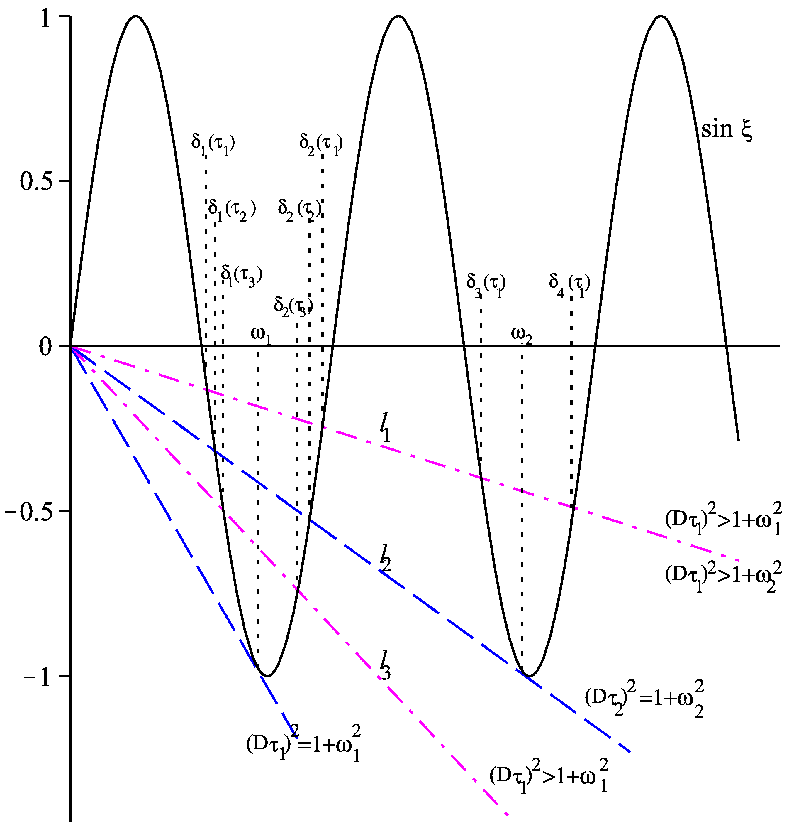
We are looking for positive solutions with respect to $\tau$ of equations (26). As in [34], we first investigate solutions of

$$sin\xi =-{\displaystyle \frac{\xi }{D\tau }},\xi \in \left((2i-1)\pi ,2i\pi \right),i=1,2,\dots ,$$

(27)

where $\xi =\tau \sqrt{F\left(\tau \right)(2D-F(\tau \left)\right)}=\tau \omega$. For any fixed $i\ge 1$ there will be a unique solution of (27) if the line $\eta =-{\displaystyle \frac{\xi }{D\tau }}$ is tangent to the curve $\eta =sin\xi$. Denote by ${\omega }_i$ this unique solution in the interval $\left((2i-1)\pi ,(4i-1)\frac{\pi }{2}\right)$, see Figure 2. Using the equality $1={sin}^2{\omega }_i+{cos}^2{\omega }_i={\displaystyle \frac{{\omega }_i^2+1}{D^2{\tau }^2}}$ and solving for $\tau$, we obtain $\tau ={\displaystyle \frac{\sqrt{{\omega }_i^2+1}}{D}}$. Clearly, if $\tau <{\displaystyle \frac{\sqrt{{\omega }_i^2+1}}{D}}$ then (27) has no solutions in the interval $\left(\right(2i-1)\pi ,2i\pi )$, and if $\tau >{\displaystyle \frac{\sqrt{{\omega }_i^2+1}}{D}}$ then there are exactly two solutions of (27) in the interval $\left(\right(2i-1)\pi ,2i\pi )$, one less than ${\omega }_i$ and one larger than ${\omega }_i$ (cf. Figure 2).

Figure 2. Solutions of $sin\xi =-\frac{\xi }{D\tau }$. The lines are $l_1:\eta =-\frac{\xi }{D{\tau }_1}$, $l_2:\eta =-\frac{\xi }{D{\tau }_2}$, and $l_3:\eta =-\frac{\xi }{D{\tau }_3}$.

Assume that $\tau \ge {\displaystyle \frac{\sqrt{{\omega }_i^2+1}}{D}}$ for some integer $i\ge 1$. Let ${\delta }_{2i-1}={\delta }_{2i-1}\left(\tau \right)$ be the unique solution of $sin\xi =-{\displaystyle \frac{\xi }{D\tau }}$ for $\xi \in ((2i-1)\pi ,{\omega }_i]$ and ${\delta }_{2i}={\delta }_{2i}\left(\tau \right)$ be the unique solution of $sin\xi =-{\displaystyle \frac{\xi }{D\tau }}$ for $\xi \in [{\omega }_i,2i\pi )$. Then ${\delta }_{2i-1}\left(\tau \right)$ is strictly decreasing, ${\delta }_{2i}\left(\tau \right)$ is strictly increasing, and (cf. [34])

$$\begin{array}{ccc}& & {\delta }_{2i-1}\left({\displaystyle \frac{\sqrt{{\omega }_i^2+1}}{D}}\right)={\delta }_{2i}\left({\displaystyle \frac{\sqrt{{\omega }_i^2+1}}{D}}\right)={\omega }_i,\hfill \end{array}$$

(28)

$$\begin{array}{ccc}& & \underset{\tau \to +\infty }{lim}{\delta }_{2i-1}\left(\tau \right)=(2i-1)\pi ,\underset{\tau \to +\infty }{lim}{\delta }_{2i}\left(\tau \right)=2i\pi .\hfill \end{array}$$

(29)

Differentiating, with respect to $\tau$, the equality

$$sin{\delta }_{2i-1}\left(\tau \right)=-{\displaystyle \frac{{\delta }_{2i-1}\left(\tau \right)}{D\tau }}$$

and using the implicit function theorem, we obtain consecutively

$$\begin{array}{ccc}\hfill & & cos{\delta }_{2i-1}\left(\tau \right){\delta }_{2i-1}^{\prime }\left(\tau \right)=-{\displaystyle \frac{{\delta }_{2i-1}^{\prime }\left(\tau \right)·D\tau -{\delta }_{2i-1}\left(\tau \right)·D}{{\left(D\tau \right)}^2}}\hfill \\ & & {\left(D\tau \right)}^{2}cos{\delta }_{2i-1}\left(\tau \right){\delta }_{2i-1}^{\prime }\left(\tau \right)=-D\tau ·{\delta }_{2i-1}^{\prime }\left(\tau \right)+{\delta }_{2i-1}\left(\tau \right)·D\hfill \\ & & {\delta }_{2i-1}^{\prime }\left(\tau \right)\left(D^2{\tau }^2·cos{\delta }_{2i-1}\left(\tau \right)+D\tau \right)={\delta }_{2i-1}\left(\tau \right)·D\hfill \\ & & {\delta }_{2i-1}^{\prime }\left(\tau \right)·\tau \left(D\tau cos{\delta }_{2i-1}\left(\tau \right)+1\right)={\delta }_{2i-1}\left(\tau \right)\hfill \\ & & {\delta }_{2i-1}^{\prime }\left(\tau \right)={\displaystyle \frac{{\delta }_{2i-1}\left(\tau \right)}{\tau \left(1+D\tau cos{\delta }_{2i-1}\left(\tau \right)\right)}}.\hfill \end{array}$$

(30)

Similarly, one obtains

$${\delta }_{2i}^{\prime }\left(\tau \right)={\displaystyle \frac{{\delta }_{2i}\left(\tau \right)}{\tau \left(1+D\tau cos{\delta }_{2i}\left(\tau \right)\right)}}.$$

(31)

Since $cos\xi$ is increasing for $\xi \in \left(\right(2i-1)\pi ,2i\pi )$, $i\ge 1$, using the relations

$${\left.cos{\delta }_{2i-1}\left(\tau \right)\right|}_{\tau =\frac{\sqrt{{\omega }_{2i-1}^2+1}}{D}}=cos{\omega }_{2i-1}=-{\left.{\displaystyle \frac{1}{D\tau }}\right|}_{\tau =\frac{\sqrt{{\omega }_{2i-1}^2+1}}{D}}=-{\displaystyle \frac{1}{\sqrt{{\omega }_{2i-1}^2+1}}},$$

we find that $cos{\delta }_{2i-1}\left(\tau \right)<cos{\omega }_{2i-1}$ for $\tau >{\displaystyle \frac{\sqrt{{\omega }_i^2+1}}{D}}$. Similarly, one can show that $cos{\delta }_{2i}\left(\tau \right)>cos{\omega }_{2i}$ for $\tau >{\displaystyle \frac{\sqrt{{\omega }_i^2+1}}{D}}$ holds true. Therefore,

$${\delta }_{2i-1}^{\prime }\left({\displaystyle \frac{\sqrt{{\omega }_i^2+1}}{D}}\right)=-\infty ,{\delta }_{2i}^{\prime }\left({\displaystyle \frac{\sqrt{{\omega }_i^2+1}}{D}}\right)=+\infty .$$

(32)

Define the function

$$G\left(\tau \right)=\tau \sqrt{F\left(\tau \right)(2D-F(\tau \left)\right)}\mathrm{for}\tau \in \left[{\tau }_{min},{\tau }_{max}\right].$$

(33)

Obviously, $G\left(\tau \right)$ is defined and nonnegative for all $\tau \in \left[{\tau }_{min},{\tau }_{max}\right]$ if and only if $F\left(\tau \right)\le 2D$ holds true. If $F\left(\tau \right)>2D$ for some values of $\tau \in ({\tau }_{min},{\tau }_{max})$, then $G\left(\tau \right)$ is not defined on the whole interval $[{\tau }_{min},{\tau }_{max}]$.

The function $G\left(\tau \right)$ plays a significant role in investigating the existence of Hopf bifurcations of $E_1$ (cf. [34]). However, since $G\left(\tau \right)=\tau \omega$, it can be used to detect other types of bifurcations of $E_1$. Indeed,

• If there exists $\overline{\tau }\in \left({\tau }_{min},{\tau }_{max}\right)$ such that $F\left(\overline{\tau }\right)=2D$, then $G\left(\overline{\tau }\right)=0$, i.e., $\overline{\omega }=\omega \left(\overline{\tau }\right)=0$. This means that $\lambda =0$ is eventually a root of the characteristic Equation (23), so that the equilibrium $E_1$ becomes nonhyperbolic at $\overline{\tau }$ leading to some kind of bifurcation.
• Since ${\mu }_{cr}^{\prime }\left(S_{cr}^{min}\right)=0$ (see (16) and (22)), it follows that $F\left({\tau }_{min}\right)=0$, and so $G\left({\tau }_{min}\right)=0$. Thus, $\tau ={\tau }_{min}$ can serve as another bifurcation value for the equilibrium $E_1$.

Theorem 1.

[34] Let $N>0$ be the largest integer such that ${\displaystyle \frac{\sqrt{{\omega }_N^2+1}}{D}}<{\tau }_{max}$ holds true. Then the following assertions are valid:

$\left(i\right)$ If $\tau ={\tau }^{*}\in \left({\tau }_{min},{\tau }_{max}\right)$ is a solution of (26), then the curve $\eta =G\left(\tau \right)$ intersects one of the curves $\eta ={\delta }_{2i-1}\left(\tau \right)$, $\eta ={\delta }_{2i}\left(\tau \right)$, $1\le i\le N$, at $\tau ={\tau }^{*}$.

$\left(ii\right)$ Let $\eta =G\left(\tau \right)$ intersects $\eta ={\delta }_{2i-1}\left(\tau \right)$ or $\eta ={\delta }_{2i}\left(\tau \right)$ at $\tau ={\tau }^{*}\in ({\tau }_{min},{\tau }_{max})$ for some $i=1,2,\dots ,N$. Then $\tau ={\tau }^{*}$ is a solution of (26), if and only if

$$\begin{array}{c}F\left({\tau }^{*}\right)\ge Dforj=2i-1,\hfill \\ \left({\delta }_j\left({\tau }^{*}\right)-\frac{(4i-1)\pi }{2}\right)\left(D-F\left({\tau }^{*}\right)\right)\ge 0forj=2i.\hfill \end{array}$$

(34)

$\left(iii\right)$ If the solutions of

$$(D-F\left(\tau \right))(\tau F^{\prime }\left(\tau \right)+G\left(\tau \right)G^{\prime }\left(\tau \right))=0,\tau \in ({\tau }_{min},{\tau }_{max})$$

(35)

are isolated, then (26) possesses a finite number of positive solutions.

The proof can be found in Appendix A.

Theorem 1$\left(i\right)$ implies that if $\eta =G\left(\tau \right)$ and $\eta ={\delta }_j\left(\tau \right)$, $1\le j\le 2N$, do not intersect for $\tau \in \left({\tau }_{min},{\tau }_{max}\right)$, then, the equilibrium $E_1$ is hyperbolic, i.e., $E_1$ does not undergo any bifurcation with respect to $\tau$.

Theorem 2.

[34] Let $\lambda \left(\tau \right)=R\left(\tau \right)+iI\left(\tau \right)$ be a root of the characteristic Equation (23) such that $R\left({\tau }^{*}\right)=0$, $I\left({\tau }^{*}\right)=\omega >0$. Then

$$sign{\displaystyle \frac{d}{d\tau }}R\left({\tau }^{*}\right)=sign\left({\tau }^{*}{F}^{\prime }\left({\tau }^{*}\right)+G\left({\tau }^{*}\right)G^{\prime }\left({\tau }^{*}\right)\right).$$

(36)

The proof is given in Appendix A.

Corollary 1.

[34] Let the assumptions of Theorem 1(i) be satisfied. Then the following assertions are valid:

$\left(i\right)$ There exists a unique integer j, $1\le j\le 2N$, $j=2i-1$, or $j=2i$ for some $1\le i\le N$, such that the curves $\eta =G\left(\tau \right)$ and $\eta ={\delta }_j\left(\tau \right)$ intersect at $\tau ={\tau }^{*}$.

$\left(ii\right)$ If $\tau \ne {\displaystyle \frac{\sqrt{{\omega }_i^2+1}}{D}}$ or $\tau \ne {\displaystyle \frac{(4i-1)\pi }{2D}}$, then

$$sign\left(\frac{d}{d\tau }R\left({\tau }^{*}\right)\right)=\left\{\begin{array}{cc}sign\left({\delta }_j^{\prime }\left({\tau }^{*}\right)-G^{\prime }\left({\tau }^{*}\right)\right),\hfill & if{\tau }^{*}\in \left({\displaystyle \frac{\sqrt{{\omega }_i^2+1}}{D}},{\displaystyle \frac{(4i-1)\pi }{2D}}\right)\hfill \\ sign\left(G^{\prime }\left({\tau }^{*}\right)-{\delta }_j^{\prime }\left({\tau }^{*}\right)\right),\hfill & otherwise.\hfill \end{array}\right.$$

(37)

The proof is presented in Appendix A.

The next theorem reports the final result on the existence of local Hopf bifurcations of the interior equilibrium $E_1$.

Theorem 3.

[34] Let ${\tau }^{*}>{\tau }_{min}$ be a solution of (26). Then the following assertions hold true:

(i) There exists a unique integer $n\ge 1$ such that $G\left({\tau }^{*}\right)={\delta }_n\left({\tau }^{*}\right)$.

(ii) If ${\tau }^{*}{F}^{\prime }\left({\tau }^{*}\right)+G\left({\tau }^{*}\right)G^{\prime }\left({\tau }^{*}\right)\ne 0$, $G^{\prime }\left({\tau }^{*}\right)\ne {\delta }_n^{\prime }\left({\tau }^{*}\right)$ where $n=2i-1$ or $n=2i$ for some integer i, $1\le i\le N$, and ${\tau }^{*}\ne {\displaystyle \frac{\sqrt{{\omega }_i^2+1}}{D}}$ or ${\tau }^{*}\ne {\displaystyle \frac{(4i-1)\pi }{2D}}$, then the equilibrium $E_1$ undergoes a Hopf bifurcation at $\tau ={\tau }^{*}$. All bifurcating periodic solutions are positive and unstable and have periods in the intervals

$$\begin{array}{ccc}& \left({\displaystyle \frac{4{\tau }^{*}}{2n+1}},{\displaystyle \frac{2{\tau }^{*}}{n}}\right),& ifnisodd;and\hfill \end{array}$$

(38)

$$\begin{array}{ccc}& \left({\displaystyle \frac{2{\tau }^{*}}{n}},{\displaystyle \frac{2{\tau }^{*}}{n-1}}\right),& ifniseven.\hfill \end{array}$$

(39)

The proof can be found in Appendix A.

2.3. The Washout Equilibrium $E_0$

For $E_0=(0,S_{ph}^0,S_{cr}^0)$ (with $X=0$), we obtain from (19) the following characteristic equation

$$D+\lambda -e^{-D\tau }{\mu }_{cr}\left(S_{cr}^0\right)e^{-\lambda \tau }=0.$$

(40)

Proposition 3.

For the model (3)–(5), the equilibrium point $E_0$ is locally asymptotically stable for $\tau >{\tau }_0$ and locally asymptotically unstable for $\tau \in (0,{\tau }_0)$.

Proof. 

Consider the characteristic Equation (40), and define the function

$$f_0\left(\lambda \right)=D+\lambda -e^{-D\tau }{\mu }_{cr}\left(S_{cr}^0\right)e^{-\lambda \tau }.$$

First, let $\tau >{\tau }_0$, or equivalently, $D>e^{-D\tau }{\mu }_{cr}\left(S_{cr}^0\right)$. We have

$$f_0\left(0\right)=D-e^{-D\tau }{\mu }_{cr}\left(S_{cr}^0\right)>0,\underset{\lambda \to -\infty }{lim}{f}_0\left(\lambda \right)=-\infty .$$

This means that there is at least one negative root of the characteristic Equation (40), thus $E_0$ is locally asymptotically stable.

In the case when $\tau <{\tau }_0$, i.e., when $D<e^{-D\tau }{\mu }_{cr}\left(S_{cr}^0\right)$, we have

$$f_0\left(0\right)<0,\underset{\lambda \to +\infty }{lim}{f}_0\left(\lambda \right)=+\infty ,$$

so there is at least one positive root of the characteristic Equation (40), which means that $E_0$ is locally asymptotically unstable. This completes the proof. □

Although the washout equilibrium $E_0$ is not of practical interest, in Section 3 we shall prove that it is also globally asymptotically stable if $\tau >{\tau }_0$. Global stability of $E_0$ means total washout of biomass in the reactor and breakdown of the degradation process.

In the same way as in [34], one can show existence of Hopf bifurcations of $E_0=(0,S_{ph}^0,S_{cr}^0)$ when it is locally unstable, i.e., for $\tau \in (0,{\tau }_0)$. In this case, due to the zero X-component, the periodic solutions bifurcating from $E_0$ cannot be nonnegative. Any periodic solution surrounding $E_0$ will involve negative and positive values, i.e., the X-component of any such periodic solution will have a zero in the interval $[t,t+\tau ]$ for certain $\tau >0$ and for any $t\ge 0$ and will change sign there. Such kinds of periodic solutions are not biologically relevant, and we skip the corresponding investigations. The interested reader can consult [34], as well as [38], for more information.

3. Global Properties of the Time-Delayed Model Solutions

Consider the time-delayed model (3)–(5). Denote by $R^{+}$ the set of all nonnegative real numbers and by $C_{\tau }^{+}$ the Banach space of continuous functions $\phi :[-\tau ,0]\to R^{+}$. Define

$$C_{\tau }^3=\{\phi =({\phi }_X,{\phi }_{ph},{\phi }_{cr})\in C_{\tau }^{+}\times C_{\tau }^{+}\times C_{\tau }^{+}\}$$

and assume that the initial data for model (3)–(5) belong to $C_{\tau }^3$.

According to the theory of functional differential equations (cf. [36,37,39]), for each $\phi \in C_{\tau }^3$ there exists a unique solution

$$\mathsf{\Phi }(\phi ;t)=(X(\phi ;t),S_{ph}(\phi ;t),S_{cr}(\phi ;t))$$

of (3)–(5) defined on $[-\tau ,+\infty )$ such that $\mathsf{\Phi }(\phi ;t)=\phi \left(t\right)$ for each $t\in [-\tau ,0]$.

Denote ${\Sigma }_1\left(t\right)=S_{ph}\left(t\right)-K{S}_{cr}\left(t\right)-S^0$, where K and $S^0$ are defined by (10). After multiplying Equation (5) by $-{\displaystyle \frac{k_{ph}}{k_{cr}}}=-K$ and adding it to Equation (4) we obtain

$$\begin{array}{ccc}\hfill \frac{d}{dt}{\Sigma }_1\left(t\right)& =& \frac{d}{dt}\left(S_{ph}\left(t\right)-K{S}_{cr}\left(t\right)\right)=D\left(S_{ph}^0-S_{ph}\left(t\right)-K{S}_{cr}^0+K{S}_{cr}\left(t\right)\right)\hfill \\ & =& D\left((S_{ph}^0-K{S}_{cr}^0)-(S_{ph}\left(t\right)-K{S}_{cr}\left(t\right))\right)\hfill \\ & =& D\left(-S_{ph}\left(t\right)+K{S}_{cr}\left(t\right)+S^0\right)=-D{\Sigma }_1\left(t\right).\hfill \end{array}$$

The latter equality means that ${\Sigma }_1\left(t\right)=e^{-Dt}{\Sigma }_1\left(0\right)$, ${\Sigma }_1\left(0\right)\ge 0$, so ${lim}_{t\to \infty }{\Sigma }_1\left(t\right)=0$. Then, system (3)–(5) can be written in the form

$$\begin{array}{ccc}\hfill \frac{d}{dt}{\Sigma }_1\left(t\right)& =& -D{\Sigma }_1\left(t\right)\hfill \\ \hfill \frac{d}{dt}X\left(t\right)& =& e^{-D\tau }\mu (S^0+K{S}_{cr}(t-\tau ),S_{cr}(t-\tau ))X(t-\tau )-DX\left(t\right)\hfill \\ \hfill \frac{d}{dt}{S}_{cr}\left(t\right)& =& -k_{cr}\mu (S^0+K{S}_{cr}\left(t\right),S_{cr}\left(t\right))X\left(t\right)+D(S_{cr}^0-S_{cr}\left(t\right)).\hfill \end{array}$$

Since ${lim}_{t\to \infty }{\Sigma }_1\left(t\right)=0$ for any $\tau \ge 0$, and we are interested in the asymptotic behavior of the dynamics, we consider the limiting system

$$\begin{array}{ccc}{\displaystyle \frac{dX\left(t\right)}{dt}}\hfill & =& e^{-D\tau }{\mu }_{cr}\left(S_{cr}(t-\tau )\right)X(t-\tau )-DX\left(t\right)\hfill \\ {\displaystyle \frac{d{S}_{cr}\left(t\right)}{dt}}\hfill & =& -k_{cr}{\mu }_{cr}\left(S_{cr}\left(t\right)\right)X\left(t\right)+D(S_{cr}^0-S_{cr}\left(t\right)),\hfill \end{array}$$

(41)

where ${\mu }_{cr}\left(S_{cr}\left(t\right)\right)=\mu (S^0+K{S}_{cr}\left(t\right),S_{cr}\left(t\right))$, cf. (12). The initial conditions for (41) belong to the set

$$C_{\tau }^2=\{\phi =({\phi }_X,{\phi }_{cr})\in C_{\tau }^{+}\times C_{\tau }^{+},S^0+K{\phi }_{cr}\ge 0\}.$$

Let us fix an arbitrary $\phi =({\phi }_X,{\phi }_{cr})\in C_{\tau }^2$, and denote ${\mathsf{\Phi }}_r(\phi ;t)=(X(\phi ;t),S_{cr}(\phi ;t))$. If no confusion arises, we shall also use the simpler notation ${\mathsf{\Phi }}_r\left(t\right)=(X\left(t\right),S_{cr}\left(t\right))$, as well as $(X\left(0\right),S_{cr}\left(0\right))$, instead of $({\phi }_X\left(0\right),{\phi }_{cr}\left(0\right))$. As mentioned before, the solution ${\mathsf{\Phi }}_r\left(t\right)$ of (41) is defined and exists for all $t\ge 0$.

Theorem 4.

$\left(i\right)$ If ${\phi }_X\left(\theta \right)=0$ for all $\theta \in [-\tau ,0]$, then $X\left(t\right)=0$ for all $t\ge 0$.

$\left(ii\right)$ Let the following inequalities be fulfilled

$$0<X\left(0\right)<{\displaystyle \frac{D{S}_{cr}^0}{k_{cr}{\mu }_{cr}\left(0\right)}}.$$

(42)

Then the solution ${\mathsf{\Phi }}_r\left(t\right)=(X\left(t\right),S_{cr}\left(t\right))$ of (41) is positive for all $t\in [-\tau ,+\infty )$ and is uniformly bounded.

Proof .

$\left(i\right)$ is obvious. The plane $X=0$ is invariant for the model (41). Therefore, we shall consider solutions $X\left(t\right)$ with ${\phi }_X\left(\theta \right)>0$ for all $\theta \in [-\tau ,0]$.

$\left(ii\right)$ Assume that $S_{cr}\left(0\right)=0$. Then, from the second equation of (41), we have

$${\displaystyle \frac{d}{dt}}{S}_{cr}\left(0\right)=-k_{cr}{\mu }_{cr}\left(0\right)X\left(0\right)+D{S}_{cr}^0>0⟺X\left(0\right)<{\displaystyle \frac{D{S}_{cr}^0}{k_{cr}{\mu }_{cr}\left(0\right)}}.$$

This implies that $S_{cr}\left(t\right)>0$ for all $t\in [-\tau ,+\infty )$.

Further, applying the variation-of-constant formula, we obtain

$$X\left(t\right)={\phi }_X\left(0\right)e^{-Dt}+e^{-D\tau }{\int }_0^t{e}^{-D(t-\sigma )}{\mu }_{cr}\left(S_{cr}(\sigma -\tau )\right)X(\sigma -\tau )d\sigma ,$$

which implies that $X\left(t\right)>0$ for each $t\in [-\tau ,+\infty )$.

Denote

$${\Sigma }_2\left(t\right)=S_{cr}^0-S_{cr}\left(t\right)-k_{cr}{e}^{D\tau }X(t+\tau ).$$

Then

$$\begin{array}{ccc}\hfill {\displaystyle \frac{d}{dt}}{\Sigma }_2\left(t\right)& =& -{\displaystyle \frac{d}{dt}}{S}_{cr}\left(t\right)-k_{cr}{e}^{-D\tau }{\displaystyle \frac{d}{dt}}X(t+\tau )\hfill \\ & =& D\left(-S_{cr}^0+S_{cr}\left(t\right)+k_{cr}{e}^{D\tau }X(t+\tau )\right)\hfill \\ & =& -{\Sigma }_2\left(t\right)\mathrm{for}\mathrm{all}t\ge 0.\hfill \end{array}$$

The latter equality implies

$$S_{cr}\left(t\right)+k_{cr}{e}^{D\tau }X(t+\tau )=S_{cr}^0+\epsilon (\phi ,t),t\ge 0,$$

(43)

where $\epsilon (\phi ,t)\to 0$ exponentially as $t\to +\infty$. This means that all nonnegative solutions are uniformly bounded and thus exist for all $t\ge 0$. The proof is completed. □

Remark 1.

Condition (42) can be explained by the complicated expression of the SKIP model $\mu (S_{ph},S_{cr})$, and, in particular, by the fact that ${\mu }_{cr}\left(0\right)$ is strongly positive (see Property (P1)). Usually, in bioreactor models, the specific growth rate $\mu (·)$ is assumed to satisfy $\mu \left(0\right)=0$. In particular, if we assume that $S_{ph}\left(0\right)=S_{cr}\left(0\right)=0$ are simultaneously fulfilled, i.e., initially the whole mixture of phenol and p-cresol is not available in the bioreactor, then condition (42) is not necessary, and it can be proved as above that all model solutions are strongly positive and uniformly bounded for all time $t\ge 0$.

The equilibrium points $E_0$, $E_1$, and $E_2$ of the reduced model (41) take the form

$$E_0^r=(0,S_{cr}^0),E_1^r=(X^{\left(1\right)},S_{cr}^{\left(1\right)}),E_2^r=(X^{\left(2\right)},S_{cr}^{\left(2\right)})\mathrm{with}{S}_{cr}^{\left(1\right)}<S_{cr}^{\left(2\right)}.$$

In what follows, we prove that the interior equilibrium point $E_2^r=E_2^r\left(\tau \right)=(X^{\left(2\right)},S_{cr}^{\left(2\right)})$ is globally asymptotically stable whenever it exists, i.e., for $\tau \in ({\tau }_{min},{\tau }_0)$.

Lemma 1.

Let $(X\left(t\right),S_{cr}\left(t\right))$ be a positive solution of (41). If $\tau \in ({\tau }_{min},{\tau }_0)$, then there exists time $T_0>0$ such that $S_{cr}\left(t\right)<S_{cr}^0$ for all $t\ge T_0$.

Proof. 

Let $\tau \in ({\tau }_{min},{\tau }_0)$. Assume that there exists time $T_0>0$ such that $S_{cr}\left(t\right)\ge S_{cr}^0$ for all $t>T_0$. Then

$${\displaystyle \frac{d}{dt}}{S}_{cr}\left(t\right)=-k_{cr}{\mu }_{cr}\left(S_{cr}\left(t\right)\right)X\left(t\right)+D(S_{cr}^0-S_{cr}\left(t\right))<0,$$

thus, $S_{cr}\left(t\right)$ is a strictly decreasing function. Since $\frac{d}{dt}{S}_{cr}\left(t\right)$ is uniformly continuous in $[-\tau ,+\infty )$, applying Barbălat’s Lemma [40], we obtain

$$0=\underset{t\to \infty }{lim}{\displaystyle \frac{d}{dt}}{S}_{cr}\left(t\right)=\underset{t\to \infty }{lim}\left[-k_{cr}{\mu }_{cr}\left(S_{cr}\left(t\right)\right)X\left(t\right)+D(S_{cr}^0-S_{cr}\left(t\right))\right].$$

Since $S_{cr}^0\le S_{cr}\left(t\right)$ and $X\left(t\right)>0$, the above equality implies that $S_{cr}\left(t\right)\downarrow S_{cr}^0$ and $X\left(t\right)\downarrow 0$ as $t\to \infty$. Define the function (cf. Lemma 2.2 in [26])

$$Z\left(t\right)=X\left(t\right)+e^{-D\tau }{\int }_{t-\tau }^{\tau }{\mu }_{cr}\left(S_{cr}\left(\sigma \right)\right)X\left(\sigma \right)d\sigma .$$

(44)

Then

$$\begin{array}{ccc}\hfill \frac{d}{dt}Z\left(t\right)& =& \frac{d}{dt}X\left(t\right)+e^{-D\tau }\left[{\mu }_{cr}\left(S_{cr}\left(t\right)\right)X\left(t\right)-{\mu }_{cr}\left(S_{cr}(t-\tau )\right)X(t-\tau )\right]\hfill \\ & =& e^{-D\tau }{\mu }_{cr}\left(S_{cr}(t-\tau )\right)X(t-\tau )-DX\left(t\right)\hfill \\ & & +e^{-D\tau }{\mu }_{cr}\left(S_{cr}\left(t\right)\right)X\left(t\right)-e^{-D\tau }{\mu }_{cr}\left(S_{cr}(t-\tau )\right)X(t-\tau )\hfill \\ & =& X\left(t\right)\left[-D+e^{-D\tau }{\mu }_{cr}\left(S_{cr}\left(t\right)\right)\right]\hfill \\ & =& e^{-D\tau }X\left(t\right)\left[{\mu }_{cr}\left(S_{cr}\left(t\right)\right)-D{e}^{D\tau }\right].\hfill \end{array}$$

(45)

Since, in this case, $D{e}^{D\tau }<D{e}^{D{\tau }_0}={\mu }_{cr}\left(S_{cr}^0\right)<{\mu }_{cr}\left(S_{cr}\left(t\right)\right)$, we find that $\frac{d}{dt}Z\left(t\right)>0$ for all sufficiently large $t>0$. So, there exists $Z^{*}>0$ such that $Z\left(t\right)\uparrow Z^{*}$ as $t\to \infty$. However, this is impossible according to the definition of $Z\left(t\right)$, and because we have already shown that $X\left(t\right)\downarrow 0$ as $t\to \infty$. Hence, there exists a sufficiently large time $T_0>0$ such that $S_{cr}\left(T_0\right)\le S_{cr}^0$. Moreover, if there exists $t_0\ge T_0$ such that $S_{cr}\left(t_0\right)=S_{cr}^0$ then

$${\displaystyle \frac{d}{dt}}{S}_{cr}\left(t_0\right)=-k_{cr}{\mu }_{cr}\left(S_{cr}\left(t_0\right)\right)X\left(t_0\right)+D(S_{cr}^0-S_{cr}\left(t_0\right))=-k_{cr}{\mu }_{cr}\left(S_{cr}\left(t_0\right)\right)X\left(t_0\right)<0.$$

The last inequality shows that $S_{cr}\left(t\right)<S_{cr}^0$ for all $t\ge T_0$. The proof is completed. □

Lemma 2.

Let $(X\left(t\right),S_{cr}\left(t\right))$ be a positive solution of (41) and $E_2^r=(X^{\left(2\right)},S_{cr}^{\left(2\right)})$ be its interior equilibrium point. Denote

$$\begin{array}{c}{\alpha }_1=lim\underset{t\to \infty }{inf}X\left(t\right),{\alpha }_2=lim\underset{t\to \infty }{sup}X\left(t\right)\hfill \\ V\left(t\right)=e^{-D\tau }{S}_{cr}\left(t\right)+k_{cr}X(t+\tau )\hfill \\ {\beta }_1=lim\underset{t\to \infty }{inf}V\left(t\right),{\beta }_2=lim\underset{t\to \infty }{sup}V\left(t\right).\hfill \end{array}$$

Then ${\alpha }_1={\alpha }_2>0$ and ${\beta }_1={\beta }_2$ hold true.

Proof. 

Assume that ${\alpha }_1=0$. Choose an arbitrary

$$\epsilon \in \left(0,{\displaystyle \frac{S_{cr}^0-S_{cr}^{\left(2\right)}}{1+k_{cr}{e}^{D\tau }}}\right).$$

According to Theorem 4 (see (43)), there exists time $T_{\epsilon }>0$ such that for all $t\ge T_{\epsilon }$ the following inequalities hold true

$$S_{cr}^0-\epsilon <S_{cr}(t-\tau )+k_{cr}{e}^{D\tau }X\left(t\right)<S_{cr}^0+\epsilon .$$

(46)

Lemma 1 implies that there exists time $T_0>0$ such that $S_{cr}\left(t\right)<S_{cr}^0$ for all $t\ge T_0$. Since ${\alpha }_1=0$, there exists $t_0>max\{T_{\epsilon },T_0\}$ such that $X\left(t\right)<\epsilon$ for all $t\ge t_0$. We set (cf. Lemma 3.5 in [26])

$$\begin{array}{ccc}\hfill \sigma & =& min\{X\left(t\right):t\in [t_0-\tau ,t_0]\},\hfill \\ \hfill \overline{t}& =& sup\{t\ge t_0-\tau :X\left(\tilde{\tau }\right)\ge \sigma \mathrm{for}\mathrm{all}\tilde{\tau }\in [t_0-\tau ,t]\}.\hfill \end{array}$$

Then $\sigma \in (0,\epsilon ]$, $\overline{t}\in [t_0,+\infty )$, $X\left(t\right)\ge \sigma$ for all $t\in [t_0-\tau ,\overline{t}]$, and

$$X\left(\overline{t}\right)=\sigma ,{\displaystyle \frac{d}{dt}}X\left(\overline{t}\right)\le 0.$$

(47)

From (46) and the choice of $\epsilon$ we obtain

$$S_{cr}^0>S_{cr}(\overline{t}-\tau )\ge S_{cr}^0-k_{cr}{e}^{D\tau }X\left(\overline{t}\right)-\epsilon \ge S_{cr}^0-(1+k_{cr}{e}^{D\tau })\epsilon >S_{cr}^{\left(2\right)}$$

and further, taking into account the monotonicity of ${\mu }_{cr}$ (Property (P2)), it follows

$$\begin{array}{c}{\displaystyle \frac{d}{dt}}X\left(\overline{t}\right)=e^{-D\tau }{\mu }_{cr}\left(S_{cr}(\overline{t}-\tau )\right)X(\overline{t}-\tau )-DX\left(\overline{t}\right)\hfill \\ >e^{-D\tau }{\mu }_{cr}\left(S_{cr}^{\left(2\right)}\right)X(\overline{t}-\tau )-DX\left(\overline{t}\right)>e^{-D\tau }D{e}^{D\tau }\sigma -D\sigma =D\sigma -D\sigma =0.\hfill \end{array}$$

The last equality contradicts (47), which means that ${\alpha }_1>0$.

Assume now that $\alpha ={\alpha }_1={\alpha }_2>0$, i.e., that the limit of $X\left(t\right)$ exists as $t\to \infty$. We shall show that ${\beta }_1={\beta }_2$ holds true. By Barbălat’s Lemma, we obtain that ${lim}_{t\to \infty }\frac{d}{dt}X\left(t\right)=0$, i.e.,

$$e^{-D\tau }{\mu }_{cr}\left(S_{cr}(t-\tau )\right)X(t-\tau )-DX\left(t\right)\to 0\mathrm{as}t\to \infty .$$

It follows then that ${\mu }_{cr}\left(S_{cr}\left(t\right)\right)\to D{e}^{D\tau }$ as $t\to \infty$, which means that $S_{cr}\left(t\right)\to S_{cr}^{\left(2\right)}$ as $t\to \infty$ and thus

$$V\left(t\right)=e^{-D\tau }{S}_{cr}\left(t\right)+k_{cr}X(t+\tau )\to e^{-D\tau }{S}_{cr}^{\left(2\right)}+k_{cr}\alpha \mathrm{as}t\to \infty .$$

Hence, if $\alpha ={\alpha }_1={\alpha }_2>0$, then ${\beta }_1={\beta }_2$ holds true.

Now assume that ${\beta }_1={\beta }_2$, i.e., the limit of $V\left(t\right)$ exists as $t\to \infty$. We shall show that ${\alpha }_1={\alpha }_2$ is fulfilled. Applying Barbălat’s Lemma yields ${lim}_{t\to \infty }\frac{d}{dt}V\left(t\right)=0$, i.e.,

$$0=\underset{t\to \infty }{lim}{\displaystyle \frac{d}{dt}}V\left(t\right)=D\left(e^{-D\tau }{S}_{cr}^0-V\left(t\right)\right),$$

which means that

$$\underset{t\to \infty }{lim}V\left(t\right)=e^{-D\tau }{S}_{cr}^0.$$

From here, it follows that there exists the limit of $X\left(t\right)$ as $t\to \infty$, i.e., ${\alpha }_1={\alpha }_2$ is satisfied.

Next, we show that the equalities ${\alpha }_1={\alpha }_2$ and ${\beta }_1={\beta }_2$ are simultaneously fulfilled. Thus, we shall use some ideas from the proofs of Lemma 4.3 in [26] and Theorem 3.1 in [27].

Let $\epsilon >0$ be an arbitrary fixed number. The Fluctuation Lemma [41] implies that there exists a sequence ${\left\{t_m\right\}}_{m=1}^{\infty }\to \infty$ such that for each m we have

$$\underset{m\to \infty }{lim}X\left(t_m\right)={\alpha }_2,{\displaystyle \frac{d}{dt}}X\left(t_m\right)=0andX(t_m-\tau )\le {\alpha }_2+\epsilon .$$

The equality $\frac{d}{dt}X\left(t_m\right)=0$ leads to

$$\begin{array}{c}{e}^{-D\tau }{\mu }_{cr}\left(S_{cr}(t_m-\tau )\right)=e^{-D\tau }{\mu }_{cr}\left({\displaystyle \frac{V(t_m-\tau )-k_{cr}X\left(t_m\right)}{e^{-D\tau }}}\right)\hfill \\ ={\displaystyle \frac{DX\left(t_m\right)}{X(t_m-\tau )}}\ge {\displaystyle \frac{D{\alpha }_2}{{\alpha }_2+\epsilon }};\hfill \\ ⟹lim\underset{m\to \infty }{inf}{e}^{-D\tau }{\mu }_{cr}\left({\displaystyle \frac{V(t_m-\tau )-k_{cr}X\left(t_m\right)}{e^{-D\tau }}}\right)\ge {\displaystyle \frac{D{\alpha }_2}{{\alpha }_2+\epsilon }}.\hfill \end{array}$$

Since $\epsilon >0$ can be arbitrarily small, it follows that

$$lim\underset{m\to \infty }{inf}{e}^{-D\tau }{\mu }_{cr}\left({\displaystyle \frac{V(t_m-\tau )-k_{cr}X\left(t_m\right)}{e^{-D\tau }}}\right)\ge D.$$

The latter inequality yields

$$lim\underset{m\to \infty }{inf}{\displaystyle \frac{V(t_m-\tau )-k_{cr}X\left(t_m\right)}{e^{-D\tau }}}\in [S_{cr}^{\left(2\right)},S_{cr}^0),$$

and hence

$${\beta }_2\ge e^{-D\tau }{S}_{cr}^{\left(2\right)}+k_{cr}{\alpha }_2.$$

(48)

Similarly, one can show that ${\beta }_1\le e^{-D\tau }{S}_{cr}^{\left(2\right)}+k_{cr}{\alpha }_1$. This and (48) lead to

$${\beta }_2-{\beta }_1\ge k_{cr}({\alpha }_2-{\alpha }_1)\ge 0.$$

(49)

Applying the Fluctuation Lemma again, there exists a sequence ${\left\{t_k\right\}}_{k=1}^{\infty }\to \infty$ such that for each k we have

$$\underset{k\to \infty }{lim}V\left(t_k\right)={\beta }_2\mathrm{and}\frac{d}{dt}V\left(t_k\right)=0.$$

Then

$$0=\frac{d}{dt}V\left(t_k\right)=D\left(e^{-D\tau }{S}_{cr}^0-V\left(t_k\right)\right),$$

and therefore

$$V\left(t_k\right)=e^{-D\tau }{S}_{cr}^0\ge {\beta }_2.$$

In the same way one can show that

$$e^{-D\tau }{S}_{cr}^0\le {\beta }_1.$$

Hence, ${\beta }_2-{\beta }_1\le 0$ holds true. This and (49) lead to ${\beta }_1={\beta }_2$. Using (49) again, we find that ${\alpha }_1={\alpha }_2$ is valid. The proof is completed. □

Theorem 5.

Let $\tau \in ({\tau }_{min},{\tau }_0)$ and $\phi \in C_{\tau }^2$ be an arbitrary element with $\phi \left(0\right)>0$ such that (42) is fulfilled. Then, the corresponding positive solution ${\mathsf{\Phi }}_r\left(t\right)=(X\left(t\right),S_{cr}\left(t\right))$ converges asymptotically towards $E_2^r=(X^{\left(2\right)},S_{cr}^{\left(2\right)})$.

Proof. 

Lemmas 1 and 2 imply that the solution ${\mathsf{\Phi }}_r\left(t\right)$ is convergent as $t\to \infty$. Let ${lim}_{t\to \infty }X\left(t\right)=X^{*}$, ${lim}_{t\to \infty }{S}_{cr}\left(t\right)=S_{cr}^{*}$. Applying Barbălat’s Lemma, we obtain

$$\begin{array}{ccc}\hfill 0& =& \underset{t\to \infty }{lim}{\displaystyle \frac{d}{dt}}X\left(t\right)=\underset{t\to \infty }{lim}\left[e^{-D\tau }{\mu }_{cr}\left(S_{cr}(t-\tau )\right)X(t-\tau )-DX\left(t\right)\right]\hfill \\ \hfill 0& =& \underset{t\to \infty }{lim}{\displaystyle \frac{d}{dt}}{S}_{cr}\left(t\right)=\underset{t\to \infty }{lim}\left[-k_{cr}{\mu }_{cr}\left(S_{cr}\left(t\right)\right)X\left(t\right)+D(S_{cr}^0-S_{cr}\left(t\right))\right],\hfill \end{array}$$

and hence

$$\begin{array}{ccc}\hfill 0& =& e^{-D\tau }{\mu }_{cr}\left(S_{cr}^{*}\right)X^{*}-D{X}^{*}\hfill \\ \hfill 0& =& -k_{cr}{\mu }_{cr}\left(S_{cr}^{*}\right)X^{*}+D(S_{cr}^0-S_{cr}^{*}).\hfill \end{array}$$

From here, it follows that $(X^{*},S_{cr}^{*})=(X^{\left(2\right)},S_{cr}^{\left(2\right)})=E_2^r$, because $E_2^r$ is the locally asymptotically stable equilibrium for $\tau \in ({\tau }_{min},{\tau }_0)$ according to Proposition 1. The proof is completed. □

The next Theorem 6 proves that the locally asymptotically stable washout equilibrium $E_0$ is also globally asymptotically stable. The proof uses similar ideas to Theorem 2.3 of [26].

Theorem 6.

Let $\tau >{\tau }_0$ and $\phi \in C_{\tau }^2$ be an arbitrary element such that (42) is fulfilled. Then the corresponding positive solution ${\mathsf{\Phi }}_r\left(t\right)=(X\left(t\right),S_{cr}\left(t\right))$ of (41) converges asymptotically towards $E_0^r=(0,S_{cr}^0)$.

Proof. 

Let $\tau >{\tau }_0$. According to the definition of ${\tau }_0$, this means that $D{e}^{D\tau }>{\mu }_{cr}\left(S_{cr}^0\right)$.

Suppose that $S_{cr}\left(t\right)<S_{cr}^0$ for all sufficiently large t. Then using the function $Z\left(t\right)$ in (44) we obtain from (45)

$$\begin{array}{ccc}\hfill \frac{d}{dt}Z\left(t\right)& =& e^{-D\tau }X\left(t\right)\left[{\mu }_{cr}\left(S_{cr}\left(t\right)\right)-D{e}^{D\tau }\right]\hfill \\ & \le & e^{-D\tau }X\left(t\right)\left[{\mu }_{cr}\left(S_{cr}^0\right)-D{e}^{D\tau }\right]\le 0.\hfill \end{array}$$

The last inequality follows from the fact that ${\mu }_{cr}\left(S_{cr}\right)$ is an increasing function for $S_{cr}\le S_{cr}^0$. Therefore, $Z\left(t\right)\downarrow \overline{Z}$ as $t\to \infty$ for some $\overline{Z}\ge 0$. Since $Z\left(t\right)$ is bounded and uniformly continuous, it follows by Barbălat’s Lemma [40] that $\frac{d}{dt}Z\left(t\right)\to 0$ as $t\to \infty$, i.e.,

$$\underset{t\to \infty }{lim}X\left(t\right)\left[{\mu }_{cr}\left(S_{cr}\left(t\right)\right)-D{e}^{D\tau }\right]=0.$$

Assume that there is a sequence $\left\{t_m\right\}\to \infty$ such that ${lim}_{m\to \infty }X\left(t_m\right)=\overline{X}>0$. Then ${lim}_{m\to \infty }{\mu }_{cr}\left(S_{cr}\left(t_m\right)\right)=D{e}^{D\tau }>{\mu }_{cr}\left(S_{cr}^0\right)$, which implies that $S_{cr}\left(t_m\right)\ge S_{cr}^0$, a contradiction. Therefore, $S_{cr}\left(t\right)\ge S_{cr}^0$ for all sufficiently large t.

Assume that $S_{cr}\left(t\right)>S_{cr}^0$ for all sufficiently large $t>0$. Then it follows from the second equation of (41) that $\frac{d}{dt}{S}_{cr}\left(t\right)<0$ for all large t, which implies that $S_{cr}\left(t\right)\downarrow {\overline{S}}_{cr}$ for some ${\overline{S}}_{cr}\ge S_{cr}^0$. If ${\overline{S}}_{cr}>S_{cr}^0$, then

$$\begin{array}{ccc}\hfill \frac{d}{dt}Z\left(t\right)& =& e^{-D\tau }X\left(t\right)\left[{\mu }_{cr}\left(S_{cr}\left(t\right)\right)-D{e}^{D\tau }\right]\hfill \\ & <& e^{-D\tau }X\left(t\right)\left[{\mu }_{cr}\left(S_{cr}\left(t\right)\right)-{\mu }_{cr}\left(S_{cr}^0\right)\right]\le 0\hfill \end{array}$$

because ${\mu }_{cr}\left(S_{cr}\right)$ is decreasing for $S_{cr}>S_{cr}^0$. Therefore, $Z\left(t\right)\downarrow \overline{Z}$ as $t\to \infty$ for some $\overline{Z}\ge 0$. Barbălat’s Lemma then implies that $\frac{d}{dt}Z\left(t\right)\to 0$ as $t\to \infty$, which means that $X\left(t\right)\to 0$ leading to $S_{cr}\left(t\right)\to S_{cr}^0$ as $t\to \infty$. If ${\overline{S}}_{cr}=S_{cr}^0$, then obviously ${lim}_{t\to \infty }X\left(t\right)=0$. Therefore, $E_0^r$ is globally asymptotically stable for the model (41). The proof is completed. □

4. Numerical Simulation

Here, we illustrate the theoretical results from the previous sections on three numerical examples for different values of the parameters D and $\tau$. We use the numerical values of the model parameters in Table 1.

We notice that ${\tau }_{min}\ge 0$ if $D\le {\mu }_{cr}\left(S_{cr}^{min}\right)\approx 0.07455989538$ is fulfilled.

The next computer simulations illustrate the occurrence of Hopf bifurcations of the interior equilibrium $E_1$, investigated in Section 2.2. First we have to determine the tangent point ${\omega }_i$ of $sin\xi$ and the line $\eta =-{\displaystyle \frac{\xi }{D\tau }}$, which coincides with the unique solution of $cos\xi =-{\displaystyle \frac{1}{D\tau }}$, i.e., with the unique solution of $tan\xi =\xi$ in the interval $\left((2i-1)\pi ,(4i-1)\frac{\pi }{2}\right)$ for some $i\ge 1$ (cf. [34]). We obtain the following values

$${\omega }_1=4.493409458\in \left(\pi ,\frac{3\pi }{2}\right),{\omega }_2=10.90412166\in \left(3\pi ,\frac{7\pi }{2}\right).$$

Example 1.

$D=0.0005$

For this value of D we obtain

$$\begin{array}{c}{\tau }_{min}=\mathrm{10,009.49990},{\tau }_0=\mathrm{10,306.76779},{\tau }_{max}=\mathrm{10,583.24050},\hfill \\ {\tau }_b:={\displaystyle \frac{\sqrt{{\omega }_1^2+1}}{D}}=9206.677698,\hfill \end{array}$$

thus, ${\tau }_{min}>{\tau }_b$ holds true. According to Theorem 1, we have $N=1$, thus, there are two solutions ${\delta }_1\left(\tau \right)$ and ${\delta }_2\left(\tau \right)$, and the equilibrium $E_1$ undergoes Hopf bifurcations at the following four values of $\tau$:

$${\tau }_1^{*}=\mathrm{10,022.86},{\tau }_2^{*}=\mathrm{10,050.78},{\tau }_3^{*}=\mathrm{10,084.7},{\tau }_4^{*}=\mathrm{10,113.52}.$$

Figure 3 visualizes the curve $G\left(\tau \right)$ and the solutions ${\delta }_1\left(\tau \right)$ and ${\delta }_2\left(\tau \right)$ as well as the above intersection points.

Figure 3. Graph of the function $G\left(\tau \right)$ and of the solutions ${\delta }_i\left(\tau \right)$, $i=1,2$.

We take $\tau ={\tau }_1^{*}=10022.86$. At this value of the delay, the two interior steady states are

$$\begin{array}{c}{E}_1=E_1\left({\tau }_1^{*}\right)=(0.0003071390889,0.1605423590,0.03257655402),\hfill \\ E_2=E_2\left({\tau }_1^{*}\right)=(0.0002781194773,0.2115122674,0.05784368812).\hfill \end{array}$$

According to Proposition 2, $E_1$ is locally asymptotically unstable for all $\tau \in ({\tau }_{min},{\tau }_{max})$. Theorem 5 implies that the equilibrium $E_2$ is globally asymptotically stable for $\tau \in ({\tau }_{min},{\tau }_0)$.

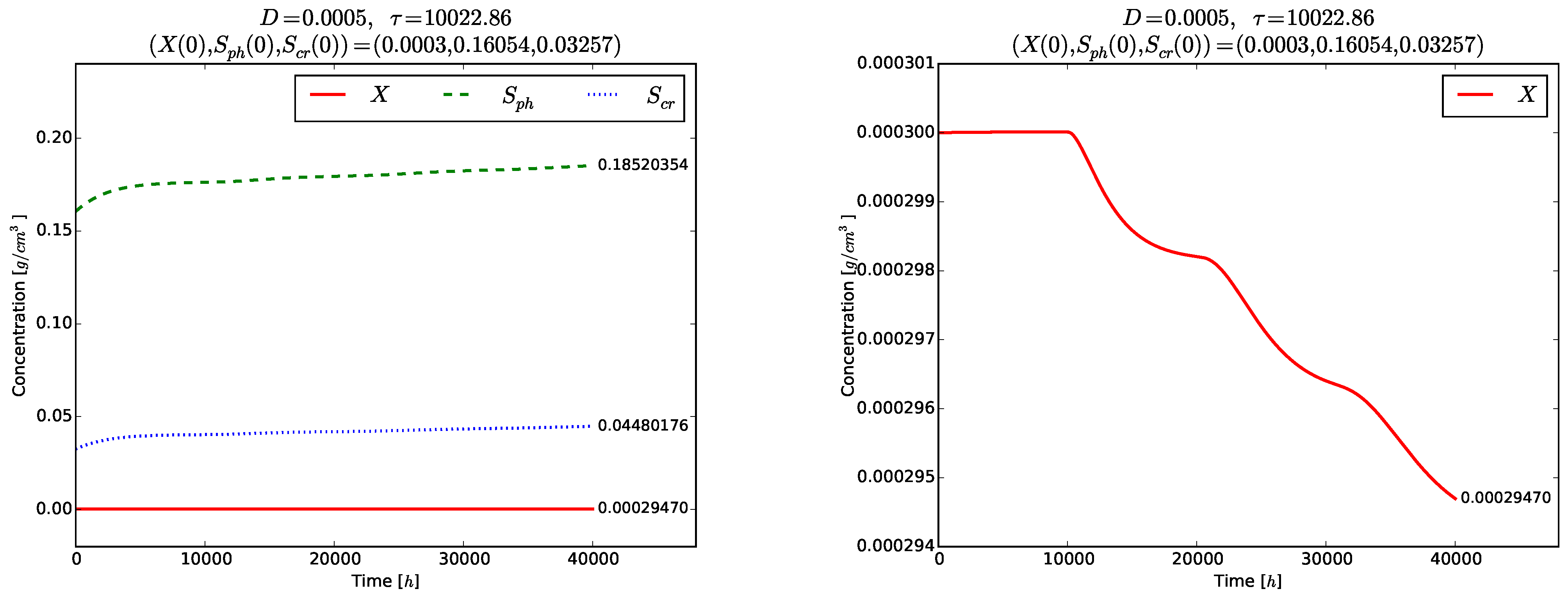
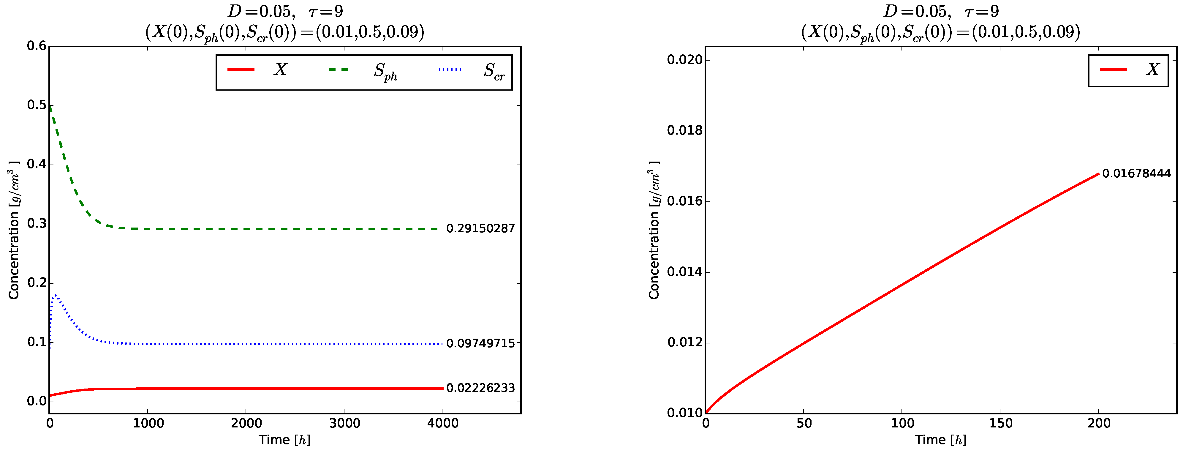
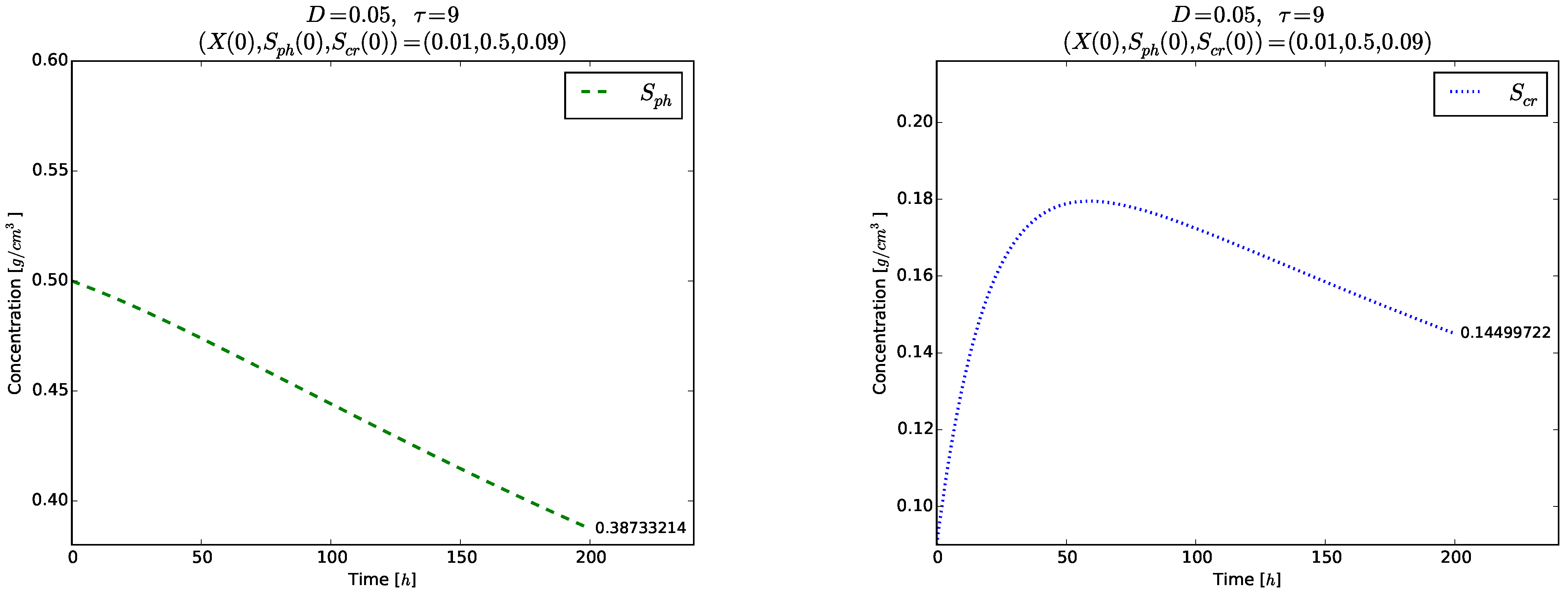
Figure 4 and Figure 5 show the time evolution of the solutions of the model (3)–(5). Although the initial conditions $(X\left(0\right),S_{ph}\left(0\right),S_{cr}\left(0\right))=(0.0003,0.16054,0.03257)$ are chosen near to $E_1$, the solutions tend to the globally asymptotically stable equilibrium $E_2$. Transient oscillations in the time evolution of the phase $X\left(t\right)$, $S_{ph}\left(t\right)$ and $S_{cr}\left(t\right)$ are observed in the right plot of Figure 4 and in Figure 5.

Figure 4. Example 1. Left plot: solutions $(X\left(t\right),S_{ph}\left(t\right),S_{cr}\left(t\right))$ of (3)–(5). Right plot: transient oscillations of the phase variable $X\left(t\right)$.

Figure 5. Example 1. Transient oscillations of the phase variables $S_{ph}\left(t\right)$ (left) and $S_{cr}\left(t\right)$ (right).

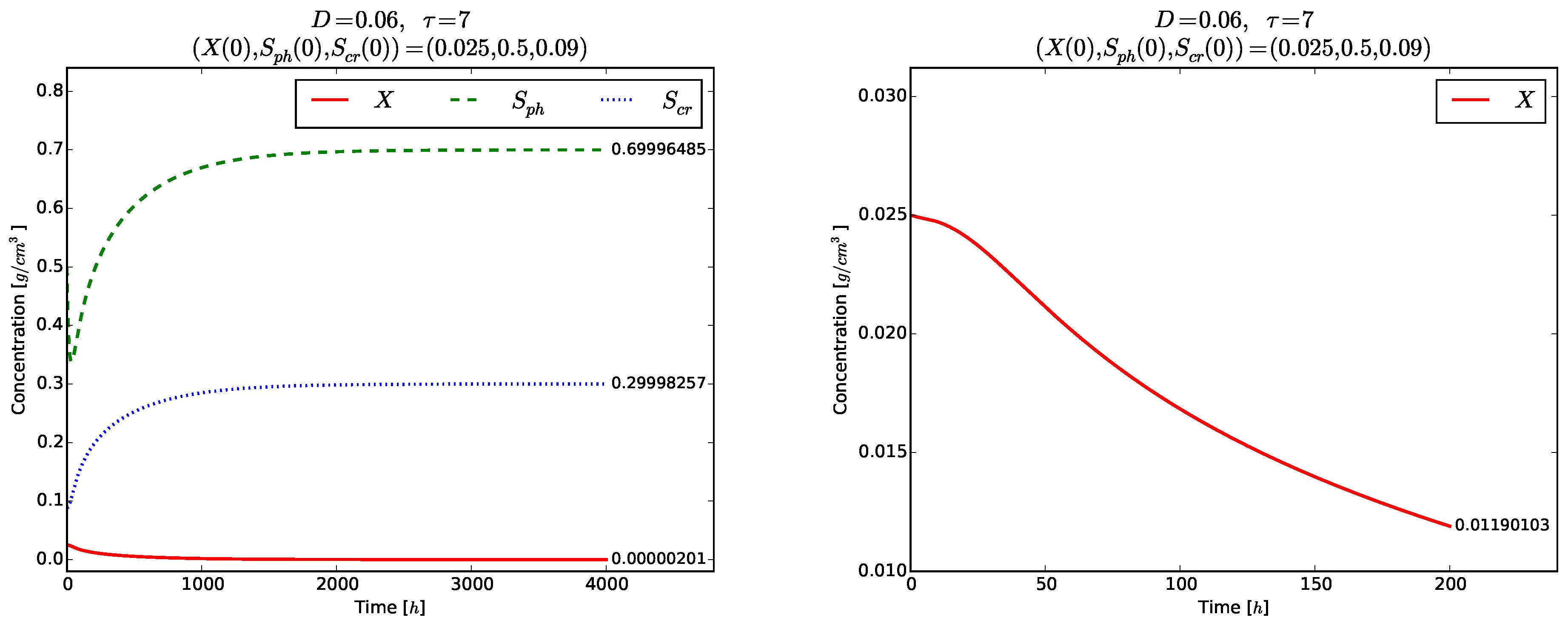
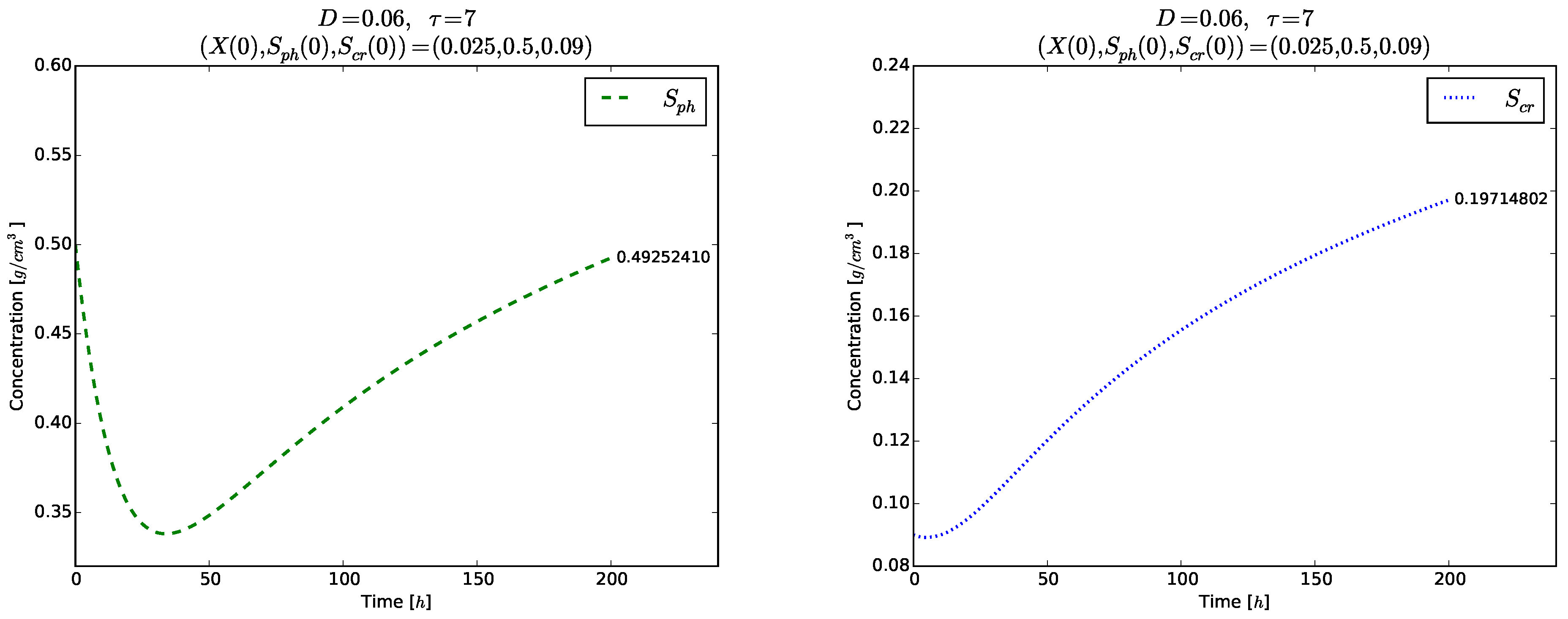
The next two examples demonstrate the global stability of the equilibrium points $E_2$ and $E_0$ with respect to D and $\tau$.

Example 2.

$D=0.05$

For this value of D we obtain

$${\tau }_{min}=7.991595294,{\tau }_0=10.96427421,{\tau }_{max}=13.72900131.$$

We choose and fix $\tau =9\in ({\tau }_{min},{\tau }_0)$. Then, there exist the two interior equilibria

$$\begin{array}{c}{E}_1=(0.03095223849,0.1320495584,0.01845191786),\hfill \\ E_2=(0.02226233088,0.2915028678,0.09749714815).\hfill \end{array}$$

Proposition 2 implies that $E_1$ is locally asymptotically unstable, and $E_2$ is the global attractor for the model (3)–(5) according to Theorem 5.

According to Theorem 4(ii) the inequality

$$X\left(0\right)<{\displaystyle \frac{D{S}_{cr}^0}{k_{cr}{\mu }_{cr}\left(0\right)}}\approx 0.02603585149$$

should be fulfilled to ensure existence of positive model solutions. The right plot in Figure 6 visualizes the time evolution of $(X\left(t\right),S_{ph}\left(t\right),S_{cr}\left(t\right))$ towards the globally asymptotically stable equilibrium $E_2$. As expected, no oscillations are observed in the time evolution of each one of the variables $X\left(t\right)$ (right plot in Figure 6), as well as of $S_{ph}\left(t\right)$ and $S_{cr}\left(t\right)$ even for the short time $t\in [0,200]$, Figure 7.

Figure 6. Example 2. Global stability of the equilibrium point $E_2$ (left). Time evolution of the phase variable $X\left(t\right)$ for $t\in [0,200]$ (right).

Figure 7. Example 2. Time evolution of the phase variables $S_{ph}\left(t\right)$ (left) and $S_{cr}\left(t\right)$ for $t\in [0,200]$ (right).

Example 3.

$D=0.06$

Here we have

$${\tau }_{min}=3.620970124,{\tau }_0=6.098202568,{\tau }_{max}=8.402141813.$$

Taking $\tau =7>{\tau }_0$ we obtain

$$\begin{array}{c}{E}_0=(0,0.7,0.3)(\mathrm{with}X=0),\hfill \\ E_1=(0.03354087904,0.1027392369,0.003922014857).\hfill \\ E_2\mathrm{does}\mathrm{not}\mathrm{exist}.\hfill \end{array}$$

In this case, $E_0$ is the global attractor of the model (Theorem 6), and $E_1$ is locally asymptotically unstable (Proposition 2).

According to Theorem 4$\left(ii\right)$, the inequality

$$X\left(0\right)<{\displaystyle \frac{D{S}_{cr}^0}{k_{cr}{\mu }_{cr}\left(0\right)}}\approx 0.03124302179.$$

has to be satisfied so that the model (3)–(5) possesses positive solutions. The left plot in Figure 8 illustrates the global stability of the washout equilibrium $E_0$. The right plot of Figure 8 and Figure 9 show the evolution of each phase variable $X\left(t\right)$, $S_{ph}\left(t\right)$, $S_{cr}\left(t\right)$ for a shorter time $t\in [0,200]$. Again, no transient oscillations can be seen in these plots.

Figure 8. Example 3. Global stability of the equilibrium point $E_0$ (left). Time evolution of $X\left(t\right)$ for $t\in [0,200]$ (right).

Figure 9. Example 3. Time evolution of $S_{ph}\left(t\right)$ (left) and $S_{cr}\left(t\right)$ for $t\in [0,200]$ (right).

5. Conclusions and Future Work

We considered a time-delayed model, describing a phenol and 4-methylphenol (p-cresol) mixture biodegradation in a continuously stirred tank bioreactor with a SKIP specific growth rate. It was based on a previously proposed and studied dynamical model, presented in [25]. The discrete time delay $\tau >0$ was introduced in the microorganisms’ growth response to indicate the delay in the conversion of the consumed nutrient into viable biomass.

We presented the mathematical analysis of the proposed time-delayed model. First, in Section 2, the equilibrium points were determined, and their local asymptotic stability was investigated in dependence on the delay $\tau$ (and on the dilution rate D). Three equilibrium points were found, namely a boundary (washout) equilibrium $E_0=(0,S_{ph}^0,S_{cr}^0)$ with $X=0$ and two interior (coexistence) equilibria $E_1=(X^{\left(1\right)},S_{ph}^{\left(1\right)},S_{cr}^{\left(1\right)})$ and $E_2=(X^{\left(2\right)},S_{ph}^{\left(2\right)},S_{cr}^{\left(2\right)})$ with $S_{cr}^{\left(1\right)}<S_{cr}^{\left(2\right)}$. For any fixed $D>0$, values of $\tau$ were determined, $0<{\tau }_{min}<{\tau }_0<{\tau }_{max}$, and it was shown that

• $E_2$ exists and is locally asymptotically stable for $\tau \in ({\tau }_{min},{\tau }_0)$ (Proposition 1);
• $E_1$ exists and is locally asymptotically unstable for $\tau \in ({\tau }_{min},{\tau }_{max})$ (Proposition 2);
• $E_0$ exists for all $\tau >0$ and is locally asymptotically stable (unstable) if $\tau >{\tau }_0$ ($\tau <{\tau }_0$) (Proposition 3).

Then, we showed that the locally unstable equilibrium $E_1$ underwent local Hopf bifurcations at certain critical values of the delay parameter $\tau \in ({\tau }_{min},{\tau }_{max})$ (Theorems 1–3). To prove this, we exploited a known approach presented in [34]. The occurrence of some transient oscillations as a result of the Hopf bifurcations was demonstrated by Example 1 in Section 4, see Figure 4 and Figure 5. In this example, the delay $\tau$ was chosen to be at one of the four existing bifurcating values, namely $\tau ={\tau }_1^{*}=\mathrm{10,022.86}$ h, which is approximately 418 days. According to Theorem 3, the period of the bifurcating solutions lies in the interval $\left(\frac{4{\tau }_1^{*}}{3},2{\tau }_1^{*}\right)\approx (\mathrm{13,363.8},\mathrm{20,045.7})$ h, which corresponds to an interval of approximately $(557,835)$ days, with a width of 318 days. Practically, this oscillating behavior is difficult to observe, not only because the periodic solutions are unstable but also due to the rather large bifurcating periods, especially in realtime laboratory experiments.

Finally, in Section 3, we established the existence and uniqueness of positive model solutions in Theorem 4. We reduced the 3-dimensional model (3)–(5) into a limiting 2-dimensional dynamical system (41). Although the reduced model was very similar to well known bioreactor models, the main difference was in the specific properties of the SKIP function $\mu (S_{ph},S_{cr})$ and, in particular, of ${\mu }_{cr}\left(S_{cr}\right)$. We proved in Theorem 5 the global asymptotic stability of the coexistence equilibrium point $E_2$ with respect to $\tau$ whenever it exists, i.e., for $\tau \in \left({\tau }_{min},{\tau }_0\right)$. However, if $\tau >{\tau }_0$, then the washout equilibrium $E_0$ is globally asymptotically stable (Theorem 6). These results mean practically either long-term sustainability of the biodegradation process when $E_2$ is the global attractor or process breakdown due to total washout of the biomass in the reactor when $E_0$ is the global attractor. Numerical examples in Section 4 (Examples 2 and 3) confirmed the latter theoretical results.

The time delayed model (3)–(5), investigated in this paper, shows many similarities in its dynamic properties in comparison with the previously studied [25] model (1) without a time delay. These are, for example, the global attractivity of the two equilibrium points $E_2$ and $E_0$. The main difference is the existence of Hopf bifurcations around the unstable equilibria at certain critical values of $\tau$, which serve as sources of transient oscillations in practical experiments.

As mentioned before, the model parameters in Table 1 were obtained from laboratory experiments for phenol and p-cresol mixture degradation. New experimental work is planned in the future to eventually account for the time delay in the biomass growth response and the model will be validated by the new data.

The proposed model (3)–(5) could be successfully used on a bioreactor scale-up, and this is also planned in the future. It is very likely to change the values of the model parameters, which will lead to adaptation of the investigations and to new conclusions. However, the following theoretical results are independent of the particular parameter values: (i) existence of a washout steady state $E_0$ and of at least one interior (coexistence) equilibrium $E_2$; and (ii) the inversely proportional relationship between the dilution rate D and the time delay $\tau$. Generally speaking, this means that relatively large values of D and small values of $\tau$ may cause biomass washout, due to the global stability of $E_0$, and thus to process breakdown in the bioreactor. On the contrary, smaller values of D and larger values of $\tau$ lead to a stable process and biodegradation sustainability due to the global attractivity of $E_2$. Since D is the controllable input in the bioreactor, these results can be very useful for the experimenter in order to obtain answers long before the physical prototype of the actual system is built and tested.

A next step in future investigations will be to treat more complex chemical compounds involving more than two substrates. The challenging element will be the design of the biomass specific growth rate as a SKIP-type model. This could be performed in dependence on experimental results showing the activity and the mutual interaction of the involved substances.