Abstract
This paper presents the transient wave packet (TWP) technique as an efficient method for wave–ice interaction experiments. TWPs are deterministic wave groups, where both the amplitude spectrum and the associated phases are tailor-made and manipulated, being well established for efficient wave–structure interaction experiments. One major benefit of TWPs is the possibility to determine the response amplitude operator (RAO) of a structure in a single test run compared to the classical approach by investigating regular waves of different wave lengths. Thus, applying TWPs for wave–ice interaction offers the determination of the RAO of the ice at specific locations. In this context, the determination of RAO means that the ice characteristics in terms of wave damping over a wide frequency range are obtained. Besides this, the wave dispersion of the underlying wave components of the TWP can be additionally investigated between the specific locations with the same single test run. For the purpose of this study, experiments in an ice tank, capable of generating tailored waves, were performed with a solid ice sheet. Besides the generation of one TWP, regular waves of different wave lengths were generated as a reference to validate the TWP results for specific wave periods. It is shown that the TWP technique is not only applicable for wave–ice interaction investigations, but is also an efficient alternative to investigations with regular waves.
1. Introduction
The interaction of ice and waves is a very complex process involving ice mechanics and wave theory. The influencing parameters are the ice type, size, thickness, distribution and ice covered area as well as mechanical properties of the ice. The ice field affects the incoming waves and the waves have a strong influence on the ice field. The waves displace and may break the ice while the ice causes a change in wave properties due to its flexural deformation as well as attenuation of waves due to scattering, damping and frictional effects.
The effect of ice on wave propagation is related to the dispersion of the waves and can be divided into a direct effect on the wave number and the attenuation of waves due to scattering and dissipation. The presence of the ice, and therewith a changed boundary condition, alters the wave dispersion immediately compared to the open water solution, affecting wave properties in terms of wave length, group velocity and amplitude. In addition, the attenuation of the wave energy during the propagation under ice causes a decrease in the wave amplitude.
Most experimental studies related to wave–ice interaction have investigated the attenuation of waves, as field measurements are easier to obtain (e.g., [1,2,3,4]). The attenuation can be described as an exponential decay of the wave energy when passing the ice field due to wave scattering and dissipation [5,6]. The attenuation depends on the ice state and mechanical properties of the ice as well as the wave length. Short waves within a wave spectrum are scattered and damped quickly, whereby the longer waves penetrate deep into the ice field [7,8], where they can travel long distances, dissipating energy only slowly (e.g., [9,10]). However, major uncertainties exist regarding the attenuation coefficient and its dependency on ice state and temperature [5,6].
The effect on the dispersion of waves under ice is complex and also strongly depends on the ice state and temperature. Field observations have shown that the presence of ice can lead to shorter or longer waves compared to waves in open water (e.g., [9,11,12,13]). The results indicate that ice type, ice thickness and the incoming wave period affect the dispersion in different ways. Different dispersion models have been developed with increasing complexity to account for the relevant physical mechanisms—from added mass and elastic plate models to viscous-layer models. A detailed study on different dispersion models and their effects on wave length as well as the area of validity of the different models can be found in Collins III et al. [14]. Measurements of wave dispersion in ice—field measurements as well as model tests in a more controllable environment—have indicated that a distinct conclusion on which dispersion model fits best is not possible. Moreover, due to the variability of the ice state, temperature and incoming wave field in terms of wave frequencies, all dispersion models appear to be suitable for certain conditions (e.g., [15,16,17,18,19]).
Summing up, the attenuation and dispersion of waves under ice are two important interacting physical mechanisms and integral parts of the breaking up of the ice-covered sea [2,8]. Thus, exact knowledge of the physics of wave–ice interaction is indispensable for an accurate description of the dynamic processes within the marginal ice zone (MIZ). Therefore, modelling of the processes in both the long and short term is required such for questions related to climate change investigations or weather forecasts, including maintaining and predicting ship routes. Besides full-scale measurements, which give real-world insights, wave–ice investigations in the controlled environment of a test facility are essential for fundamental research. In this context, experiments exclusively focused on wave–ice interactions are a quite recent research field compared to the originally intended structure–ice investigations featuring the classical application area of ice tanks. Thus, the established model ice has been developed to physically test its interaction with structures on a small scale. Following Froude and Cauchy scaling laws, the model ice has particular mechanical properties, which are adjusted to scale the downward breaking of a ship in ice correctly (e.g., [20,21]). The adjustment is done by crystal size and added chemicals. The main objective here is the correct scaling of the global forces (resistance) on the ship, while accepting that some of the resistance components might not be scaled correctly. Generally, model ice has been developed over recent decades to overcome or reduce certain problems such as plasticity or ductility (e.g., [21,22,23]).
Although model ice might represent the force level correctly, it has a significant amount of plasticity. The latter has been shown numerically for a different model ice type (fine-grained) by von Bock und Polach [24] and on the basis of measurement data for most existing model ice types [25]. Due to the plasticity of the model ice, the ice undergoes larger deformation to reach the critical failure stress than actual ice (sea ice, lake ice) would [26,27]. Consequently, the higher proportion of plasticity in model ice is likely to affect the energy dissipation of waves underneath the ice sheet which will introduce a scale effect in terms of higher damping.
However, several wave–ice interaction experiments in the controlled environments of test facilities have been conducted in recent years, focusing either on regular waves or irregular sea states. The research questions are manifold, from fundamental research on theoretical wave–ice propagation models to ships and structures in waves. Most of the studies deal with fundamental research questions such as damping and attenuation, wave characteristics and dispersion as well as the consequences for the ice under various different ice conditions. These studies are normally conducted with regular waves, as they can be used to answer specific research questions in a clearly defined manner [16,17,18,28,29,30,31,32,33,34,35,36]. Those experiments comprise the generation of a set of regular waves to cover a wide frequency range, so that a long test campaign may affect the ice characteristics. On the one hand, the cooling control system regulates the temperature with the target to keep ice properties constant during the experiments. However, ice properties are affected by various parameters, which vary over the time of the experiments, such as water temperature, ice thickness or entrapped chemicals and, consequently, a certain dynamic or variation of the ice properties is inevitable. On the other hand, the persistent bending of the ice due to the presence of the waves may affect the micro-structure and the mechanical behaviour of the ice by various causes, such as the growth of micro-cracks and increased plasticity up to the limit of fatigue strength. This strongly implies that the ice characteristics in terms of wave damping can also change during the course of the test campaign. In consequence, the scalability of experiments is affected by both inherent ice scale effects, such as excessive plasticity, and dynamic variations of ice properties, which can also cause unintended breakup and macro-crack formation due to fatigue.
Applying transient wave packets (TWPs) for wave–ice interaction experiments can overcome this problem. TWPs [37,38,39] represent a special type of transient wave [40,41,42,43]. Transient waves and TWPs have been introduced as efficient tool for seakeeping tests [37,38,39,40,41,42,43], enabling the determination of wave length-related problems by one test run instead of time-consuming investigations with a multitude of different regular wave lengths. TWPs are tailor-made wave groups, consisting of an amplitude spectrum of a certain shape and bandwidth, and manipulated phases. The width of the spectrum can be adapted to comply with the relevant frequency range in terms of structure response. Therefore, the main assumption is that the small amplitude waves as well as the structure response following a linear system behaviour, i.e., a structure that is excited at a certain frequency, responds with exactly the same frequency. This means that energy exchange between different frequencies is neither ruled out for the wave excitation nor for the response, so that the interaction can be described by linear response amplitude operators (RAOs).
Transferring this concept to wave–ice experiments means that the TWP can be used to evaluate the attenuation of specific ice characteristics by comparing the amplitude spectrum at the different measuring points along the tank. In this context, RAOs mean that the measured vertical displacement of the ice at downstream positions of the ice field is related to the vertical displacement of the ice at the beginning of the ice field, resulting in a frequency-dependent spatial damping spectrum over a wide frequency range.
The applicability of TWPs as an efficient tool for wave–ice interaction experiments was evaluated. Experiments with a solid ice sheet were performed, including the generation of a TWP as well as a set of regular waves of a certain frequency. The regular wave results were used to evaluate the applicability of the TWP. It is shown that wave attenuation as well as wave dispersion under ice can be addressed efficiently by TWPs. The paper starts with a brief description of the theoretical background of waves travelling beneath ice. Afterwards, the test campaign, including test setup, model ice generation and the experimental programme, is presented. Finally, the results are discussed and the paper ends with concluding remarks.
2. Theoretical Basis
The theoretical basis is derived focusing on aspects relevant for this paper. Figure 1 presents the considered theoretical framework domain for the derivation of the wave equation, showing the profile of the x–z plane. The wave system is reduced to uni-directional waves, neglecting contributions in the y-direction, i.e., the waves are travelling in a positive x-direction. This assumption reflects the conditions during the model tests and reduces the complexity of the water wave problem significantly, but does not affect the general scheme of the derivation. The point of origin is at the still water level, and the positive z–axis faces upwards, opposing the gravitational force. The positive x–axis points to the direction of wave propagation.
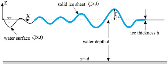
Figure 1.
Definition of the coordinate system showing the profile of the x-z plane: The point of origin is at the still water level, the positive z-axis faces upwards, opposing the gravitational force, and the positive x-axis points to the direction of wave propagation assuming uni-directional waves. Note that the wave elevation in open water and the vertical displacement of the ice are assigned the same variable , but as soon as a clear distinction has to be made between open water and ice-covered water, this is indicated by the indices i for ice and w for open water.
2.1. Open Water Waves
The theoretical basis for water waves in arbitrary water depth is presented, with the term "open" serving as a distinction from ice-covered waves in the next section. Potential theory depicts the basis for the description of the water wave problem. The fundamental assumptions are that the Newtonian fluid is inviscid, irrotational and incompressible. Thus, the fluid domain can be described by a Laplace equation,
with . The fluid domain is bounded by the bottom and the free surface. The bottom is considered to be horizontal, rigid and impermeable, and the bottom boundary condition states that the vertical velocity component must be zero at ,
with d representing the water depth. At the unknown free surface , the kinematic boundary condition,
and dynamic boundary condition,
must be fulfilled. The subscripts in Equations (1)–(4) represent the corresponding derivations. The kinematic boundary condition states that free surface particles remain at the surface regardless of whether the surface is at rest or in the presence of waves. The dynamic boundary condition ensures that the pressure at the free surface is in equilibrium with the adjacent medium. The fact that the Cauchy boundary conditions (Equations (3) and (4)) have to be fulfilled at the unknown free surface complicates the solution of the boundary value problem.
The solution can be approximated by introducing perturbation theory and Taylor series expansion for the unknown potential and surface elevation (Equations (1)–(4)). The linear solution, also known as Airy wave theory [44], is obtained by applying the perturbation parameter , which relates to the wave amplitude and the wave number , and truncation of the series expansion at order under the fundamental assumption of small amplitude waves, i.e., the wave height is significantly smaller compared to the wave length. Consequently, the analytical solution for the linear potential for arbitrary water depth is
and the plane wave solution represents the simplest form for the surface elevation. A detailed description of the derivation of the Cauchy problem, including an overview of the available solutions and approximations of different complexities, can be found in classical textbooks, e.g., [45,46,47,48].
For irregular sea states, the standard model of ocean waves can be applied, where the sea state is regarded as a superposition of independent component waves,
with , , and as amplitude, wave number, angular frequency and phase of the component wave. Equation (6) enables a simple handling of complex sea states in space and time with widely acceptable results for engineering applications. The analytical basis for the standard model of ocean waves is the Fourier transform. The spectral density of a sea state ,
represents the energy distribution as a function of angular frequency and is the frequency resolution.
The angular frequency and the wave number are linked via the dispersion relation and are affected by the dynamic boundary condition. For open water (Equation (4)), the dispersion relation is
with water depth d and gravitational acceleration g.
2.2. Ice-Covered Waves
The wave propagation in the presence of ice depends strongly on the prevailing ice characteristic regarding the structure, distribution and size and is sensitive to changing conditions (e.g., waves, wind, temperature, currents). In this context, the ice state in terms of salinity and temperature plays a significant role not only for wave propagation in ice but also regarding mechanical properties and ice breakup processes, respectively. Additionally, variations in thickness affect the effective strength and stress magnitudes in ice. Thus, different dispersion models have been developed, particularly to account for the different types of ice fields, i.e., it is of significant importance if the wave system travels along a solid or very large ice sheet, ice floe to frazil–pancake ice fields or slush ice [14].
For this study, the linear elastic thin plate theory was applied as the experiments were performed with a solid ice sheet (compared to the wave length). Assuming that the vertical displacement of the ice sheet follows the wave profile propagating under the ice, i.e., no slip condition, yields that the boundary conditions introduced above have not lost their general validity, but must be adapted to the presence of the ice [49]. Particularly, the pressure in the dynamic boundary condition must be adapted to take the static and dynamic pressure (ice deflection) of the ice sheet into account. For clarity reasons and to be consistent with the boundary value problem introduced above (Equations (1)–(3)), the vertical displacement of the ice is assigned the same variable as for the wave elevation. However, as soon as a clear distinction has to be made between open water and ice-covered water, this is indicated by the indices i for ice and w for open water. This means that a general applicability in both conditions is possible if no index is used.
The linearised dynamic boundary condition, considering bending B, inertia M and compression Q of the ice sheet, is [2,9,50]
with E as the Young’s modulus for the ice, h the ice thickness, Poisson’s ratio, P the compressive stress in the ice pack and the density. Consequently, the dispersion relation for thin elastic plate theory results in [50]
with
The parameter B denotes the plate modulus and expresses the elastic restoration of the deflected ice sheet. The compression, Q, accounts for compressive stresses due to the dynamics of the ice, which might, for instance, be introduced by wind or waves reflected at the ice edge that introduce a horizontal stress into the ice sheet. The inertia term, M, reflects the fraction of ice below the still water line.
2.3. Transient Wave Packets
Transient wave packets have been introduced for the efficient experimental determination of the hydrodynamic behaviour of ships and offshore structures e.g., [38,39,51,52,53,54,55]. TWPs are characterised by a synthesised task-related wave spectrum with tailored phase distribution. The phase distribution is adjusted in such a way that all components of the wave spectrum are in-phase superimposed at the concentration point, yielding a single wave peak. The shape and width of the spectrum can be adapted to the relevant frequency range of interest.
Generally, different shapes for the tailored wave spectrum have been introduced for transient waves in model testing. Davis and Zarnick [40] have derived a weighting function by assuming a unit impulse of wave height at a certain target location. The backwards calculated wave at the wave board featured the well-known characteristic of waves of short wave length at the beginning of the signal followed by steadily increasing wave lengths within the wave group. Mansard and Funke [42] have combined a bell-shaped modulator with a saw tooth wave, also resulting in the well-known transient wave characteristic at the wave board. Grigoropoulos et al. [43] have determined the wave board motion based on a wave spectrum with constant wave steepness, resulting in the shape of a straight line of constant slope (in the frequency domain). Gaussian wave packets are special transient waves as the wave amplitudes of the spectrum are Gaussian distributed and the propagation of the wave group can be described analytically [37]. Normalised Fourier spectrum functions have been introduced by Clauss and Kühnlein [38,39].
For this study, the following normalised Fourier spectrum function [54] was applied,
with as the lower and as the upper limit of the relevant frequency range. The phase distribution of the individual component waves of the spectrum is , which results in the in-phase superimposed single peak wave at the concentration point at . The term in the exponent is introduced in order to shift the wave group to the centre of the time frame.
To arrive at the wave group in the time domain, the inverse discrete Fourier transform (DFT) can be applied,
with the discrete time (), the number of samples , the angular frequency resolution and the sampling rate . Note that the Fourier spectrum from Equation (12) needs to be converted into a complex double-sided spectrum with the conjugate complex counterpart. The width of the complex double-sided spectrum depends on the chosen duration T of the time frame and the sampling rate f. The corresponding frequencies of the double-sided spectrum are
For the left single-sided spectrum, the frequency range for Equation (12) is . Outside this range, the left single-sided spectrum can then be zeroed before calculating the conjugate complex counterpart.
Figure 2 presents an overview of the TWP procedure. The normalised Fourier spectrum, based on Equation (12), is shown in the left diagram of Figure 2a. The normalised TWP at the concentration point, i.e., the single peak wave at , is shown in the right diagram of Figure 2a. The term "normalised" indicates that the height of the wave crest of the single peak wave is set to one. The normalised TWP in time domain is obtained by multiplying the normalised Fourier spectrum (Equation (12)) with before applying the inverse DFT ( represents the area under the normalised Fourier spectrum as shown in Figure 2a).
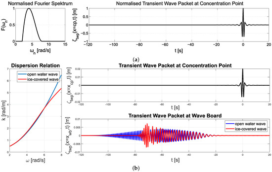
Figure 2.
Overview of the TWP concept. (a) Theoretical TWP concept—normalised TWP Fourier spectrum (left) and normalised TWP in time domain at concentration point (right). (b) Application TWP concept—TWP at concentration point (top right) and corresponding surface elevation at the wave board (bottom right). The surface elevation based on open water dispersion is shown by the blue curve and the consequences for wave propagation due to the presence of the ice sheet are illustrated by the red curve. The comparison of the dispersion relation between open water (blue curve) and the ice sheet (red curve) is shown in the left diagram.
The application of the TWP concept within this study is shown in Figure 2b. At the beginning, the height of the single peak wave crest and the position of the location of the concentration point relative to the wave board need to be defined for the calculation of the wave at the wave board and wave board motion, respectively. The aim of the present study was to explore the possibilities of the TWP concept for wave–ice interaction experiments while ensuring that the ice sheet does not break. Under this premise, the height of the single peak wave crest was set to and the distance between concentration point and wave board to (c.f. Table 1 and Equation (17)). Both the relatively small height and the chosen concentration point ensured that the TWP features only small waves under the ice sheet. In this context, it is worth noting that the length of the ice sheet (, see Figure 3) was significantly shorter than the distance from the wave board to the concentration point, i.e., the maximum crest height was defined to occur behind the ice sheet.

Table 1.
Overview on the model ice characteristics.
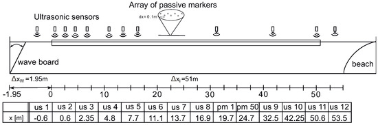
Figure 3.
Schematic sketch of the experimental test setup and positions of the sensors.
The wave at the wave board can be determined by inserting in Equation (12), which transforms the wave group linearly to the wave board. Multiplying the defined single peak wave crest height with the (normalised) TWP solutions in the time domain (at as well as ) results in the tailored TWP at the concentration point (top diagram of Figure 2b) as well as the corresponding wave at the wave board (bottom diagram of Figure 2b). To evaluate the impact of the presence of the ice sheet on the propagation of the wave group, a linear transformation was carried out for the open water (blue curve) and the ice-covered water dispersion relation (red curve, ice properties are taken from the experiments—see Table 1). Comparing both wave groups at the wave board revealed that the shape of the wave groups differed significantly and only the last part of both wave groups looked similar. This discrepancy means that the dispersion relation differs significantly for the shorter wave periods, as TWPs are generated in such a way that the generated wave length at the wave board increases with time, so that all waves arrive at the same time at the concentration point. The dispersion relation for both conditions is illustrated in the left diagram of Figure 2b, showing this difference clearly. The shorter wave periods (larger wave frequencies) result in shorter wave numbers due to the presence of the ice which means that the wave lengths increase and that the waves of shorter wave periods travel faster compared to open water. However, the TWPs generated for this study were determined based on the open water dispersion relation due to practical reasons and the fact that it did not depend on which dispersion relation was used for the purpose of this study. The main objective was to generate a tailored TWP which was neither too steep nor in phase under the ice sheet. From this point of view, using the open water TWP in ice-covered water (blue curve in the bottom graph of Figure 2b) is even more conservative as the shorter wave periods propagate much faster in the presence of the ice compared to the open water dispersion relation, hindering the in-phase superposition of all component waves at the concentration point (wave damping is left out of the discussion).
2.4. Wave Damping
Wave damping describes the energy dissipation of the waves during wave propagation. For ice-covered waves, the damping follows a frequency-dependent exponential decay
The attenuation coefficient describes the decay of the wave amplitude between two measuring points in space and represents the distance along wave propagation between these two points. For ice-covered wave spectra, the attenuation coefficient is
the index indicates the second measuring point downstream from the wave propagation and the frequency-dependent attenuation coefficient also depends on the distance of the two signals. Equation (16) depicts a classical RAO, relating two signals (output vs. input) under the assumption of linear behaviour. This underlines the motivation for exploring the TWP concept for wave–ice interaction investigations in terms of wave dispersion and damping. The Fourier transform depicts the analytical basis for this approach.
3. Experiment
The experiments were performed in the ice tank at the Hamburg Ship Model Basin (HSVA). The ice tank is suitable for a wide range of investigations. For our experiments, a fully computer controlled, electrically driven wave generator was installed on one side and a wave-damping slope on the opposite side to suppress wave reflections. A detailed description of the model ice generation procedure including the adjusted model ice properties, the experimental setup and programme is given in the following subsections.
3.1. Model Ice
The model ice at HSVA is seeded columnar ice. Once the ice tank is cooled sufficiently, spontaneous nucleation occurs, forming natural ice. This unwanted ice is removed with the carriage while spraying a fine water mist over the cooled water surface. The fine mist particles settle on the supercooled water surface and act as ice nuclei, similar to atmospheric forcing with mist or snow, from which thin ice crystals grow downwards in columnar crystals as in sea ice. The strength of the ice is adjustable due to brine entrapments from 0.7% NaCl dissolved in the tank water and added micro-air bubbles added from the bottom during growth [21,23]. The ice properties are adjusted by a cooling period to consolidate the ice and a subsequent tempering period to adjust the strength.
The ice properties—except the effective strain modulus—are measured following the guidelines of the International Towing Tank Conference, ITTC [56]. The effective strain modulus is the linear representation of the elastic modulus and the plastic strain modulus based on the flexural strength measurements. Here, the actual force displacement curve has a steep increase and a relatively long flat progression in the plastic domain until failure. The effective strain modulus linearly connects the origin and the point of failure in the force displacement curve and represents the effective stiffness of the ice that the waves experience [25]. The analysis was conducted with a linear iteration routine and a finite element model with solid elements and a element size of 4 mm for a 25.5 mm thick ice sheet based on a convergence study. Consequently, the effective strain modulus, E, was the only item of the compiled ice properties in Table 1 not directly measured.
The scaling of model scale experiments in ice is still subject to ongoing developments and discussions [27,57]. However, it is considered established that the ratio of the strain modulus (i.e., Young’s modulus in the elastic domain), E, and the bending strength, , should satisfy [21,58]. In the conducted experiments (Table 1), this ratio was significantly lower and in the range . The latter is an acknowledged scale effect that becomes significant for the breakup of ice by waves.
3.2. Experimental Setup
Figure 3 shows a schematic side view of the ice tank, including the experimental setup of the test campaign. The ice tank is long, the width is and the water depth was a constant depth of . On one side, a fully computer controlled electrically driven flap-type wave generator is installed, enabling the generation of regular waves and irregular sea states. In addition, tailored wave sequences to be defined at the wave board can also be processed by the software. On the opposite side, a beach is installed, consisting of several crossbars with space in between to suppress disturbing wave reflections. However, the measuring duration and the subsequent evaluation were designed in such a way that the influence of reflecting waves could be excluded.
The free floating ice sheet was cut free at the tank wall and had a length of . In addition, the ice sheet was moved towards the wave board to create only a small open water area of in front of the ice sheet.
The setup consisted of several active as well as passive measuring devices in order to detect the vertical displacement of the ice. Altogether, 12 ultrasonic sensors (us) were installed along the tank. All us sensors were from Ultralab, eight sensors of type 2001300 and four of type 30250. The technical details about the us sensors are provided in Table A1 in Appendix B. In addition, an array of 50 passive markers (pm) with an equal distance of were placed in the middle of the ice sheet. For this test campaign, spheres with a diameter of were used as pm, being able to reflect the invisible infrared light. The pm were positioned on the ice sheet and frozen solid, so that the surface elevation at the location of a pm equalled the pm motion. The motions of the pm were recorded by the established motion capture system Qualisys. The exact positions during the tests are provided in the table below the schematic sketch of Figure 3. For the pm array, only the first and last marker is mentioned for brevity reasons.
3.3. Experimental Programme
The experimental programme comprised the generation of one TWP and four regular waves. As already mentioned, the TWP parameters were chosen in such a way that a significant ice sheet deflection or even breaking of the ice was excluded and was
The application of the TWP technique for our experiments, based on these TWP parameters, has already been described above. In addition, the corresponding wave spectrum is shown in Figure 2a and the blue curve in Figure 2b represents the wave at the wave board used for the experiment.
The investigated regular waves comprised varying wave periods. Table 2 presents the selected parameters for the individual waves. The wave periods of the regular waves were chosen so that they were within the centre of the frequency band of the TWP. The wave steepness for the regular waves was chosen under the premise that neither large ice deflections nor ice breaking occurs. A general overview on the analysis procedure for the regular waves as well as a detailed presentation of the results is given in Appendix A.
Table 2.
Overview on the investigated four regular waves. The first table column presents the unique identifier for each regular wave, the second column the angular frequency and the last column the wave steepness.
4. Results
Figure 4 presents the experimental results for the TWP. The left diagrams show the measured vertical displacement of the ice for selected positions along the tank. The respective type and position of the measuring devices are displayed in each diagram and (cf. Equation (15)) represents the relative distance between the actual measurement position and the reference measurement at the beginning of the ice sheet (us 2, cf. Figure 3), i.e., the distance increases from top to bottom. The change in the wave group from top to bottom is obvious, resulting in a narrower wave group with increased wave height. The mechanism for this may be found in wave damping as well as in wave dispersion, and can be investigated in detail with the help of the other diagrams. The corresponding wave amplitude spectra are shown in the middle column. The different spectra already show a significant advantage of TWPs, as the clearly defined and smooth spectrum allows easy comparison of the different positions. The diagrams show that the amplitude spectrum decreases in the range of shorter wave length with increasing distance , but remains almost constant for the longer wave length.
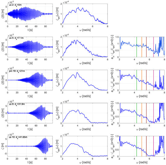
Figure 4.
Experimental results of the TWP. The diagrams on the left-hand side present the measured vertical displacement of the ice for specific locations along the tank. The centre diagrams show the corresponding amplitude spectrum and the diagrams on the right-hand side show the determined attenuation coefficient. The four coloured vertical lines in the diagrams on the right-hand side represent the position of the investigated regular waves within the TWP frequency spectrum.
The diagrams in the right column show the course of the attenuation coefficient in the frequency domain by applying Equation (16) between the amplitude spectra of the actual measurement (same row to the left) with the amplitude spectra of the reference measurement (middle top diagram). The four coloured vertical lines represent the position of the investigated regular waves within the TWP frequency spectrum.
The diagrams can be read as follows: No attenuation denotes that the wave amplitude for a certain frequency does not change, resulting in an attenuation coefficient of and everything below means that the amplitude is attenuated (values above would denote that the amplitude increases during the propagation under the ice sheet). The limiting case of means that the amplitude is cancelled out. This limiting case is difficult to evaluate as the distance and the amplitude needed to be cancelled out must not correspond with the position of the measurement, i.e., the cancellation could have happened much earlier. Another limiting case in terms of measuring accuracy is located at the boundary of the defined frequency range. On both ends, the initial amplitude spectrum is already very small, which makes this area very sensitive to measuring errors. This can be seen in the diagrams for areas and . However, it can be avoided by taking it into account during the initial selection of the frequency band, i.e., defining a wider frequency range.
The diagrams on the right hand side of Figure 4 show that the TWP technique enables the determination of the attenuation coefficient over the selected frequency range. Analysing the results in detail reveal the well-known behaviour of waves propagating in the presence of ice—the waves are damped due to the ice and the damping depends on the wave period and the propagation distance. The shortest waves () are already significantly damped at (top right diagram of Figure 4) and the longer waves are damped as well with increasing distance from top to bottom ( at ).
Figure 5a presents the comparison of the attenuation rate between the TWP and the regular waves for the four selected wave frequencies. Each diagram shows the result for one wave frequency, comparing the attenuation of the wave amplitude of the regular wave with the TWP amplitude at the corresponding specific frequency (indicated with the same colour as used for coloured vertical lines in Figure 4). The abscissa axis represents the position along the ice sheet (cf. Figure 3) and the ordinate axis represents the attenuation at the measuring positions. The first ultrasonic sensor above the ice sheet (us 2) serves as a reference. The blue plus show the results for the TWP and the stars for the regular wave. The exponential fit of the TWP is illustrated as a blue curve and the confidence interval of the exponential fit is indicated with grey lines.
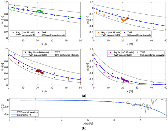
Figure 5.
Presentation of the experimentally determined attenuation and damping coefficients. The attenuation coefficient for four selected frequencies is shown in (a), comparing the results of regular waves with the TWP measurements of the same frequency. The exponential damping coefficient determined by the TWP technique is presented in (b). (a) Comparison of the attenuation coefficients for selected frequencies of the TPW (plus) and the corresponding four investigated regular waves (stars). (b) Frequency-dependent exponential damping coefficient a(wn).
Comparing the attenuation rates in detail reveals a sufficient agreement between both methods. The course of the attenuation in regular waves follows in all cases the exponential fit for the TWP, indicating the same attenuation coefficient. Nevertheless, an offset between the results for regular waves and the exponential fit of the TWP can be observed in a few cases. This difference can be attributed to the fact that the measurements at the various locations are subject to a perceptible scatter. In particular, the results of the TWP show a higher scatter along the ice sheet. Possible explanations will be addressed in the following section.
Figure 5a indicates the potential of the proposed TWP technique. It enables the determination of the frequency-dependent attenuation coefficients over a wide frequency range by one test run. The width of the frequency spectrum is predefined by the chosen TWP parameter. Thus, calculating the attenuation coefficient not only for the four frequencies shown in Figure 5a but for the whole TWP spectrum and applying Equation (15) gives the frequency-dependent exponential damping coefficient . Figure 5b illustrates the results of this calculation, the grey curve represents the computation results and the blue curve represents the exponential fit. The measurement-based course of the grey curve shows that scattering starts at approximately and leads to unusable results at approximately . The reasons for this are to be found in the measurement inaccuracies at the boundaries of the TWP spectrum. As shown in Figure 4, the measurement inaccuracies result in unrealistic values for the attenuation coefficients for , which consequently also cause incorrect results for the frequency-dependent attenuation coefficient for . However, the application of an exponential fit function between also provides appropriate results outside this range, as shown in Figure 5b.
Next, the applicability of the results using linear theory is demonstrated. Linear theory allows the transformation of the wave components to any point in space and time, e.g., (Equation (6)), but in practice, linear theory is subject to certain physical limitations. Nevertheless, it is often used in the field of ocean engineering due to its simple applicability and sufficiently accurate results over a wide application range. In contrast to waves in open water, for application to waves in ice, the ice damping must be known and taken into account for a realistic representation of the wave propagation. For the following investigation, the measured surface elevation at the beginning of the ice sheet (us 2) serves as an input wave system for the linear transformation. The discrete Fourier transformation serves as the analytical basis for the linear transformation of the measured surface elevation in the time domain at a fixed location x,
Based on this, the Fourier spectrum of the reference location can be shifted to any target position by
Taking the determined wave damping coefficient into account, Equation (19) changes to
The inverse DFT (Equation (13)) of the shifted Fourier spectrum gives the surface elevation at the desired location in the time domain.
Figure 6 shows measured surface elevations and the respective linear transformations for three selected locations along the tank. The propagation distances increase from top to bottom. Each diagram on the left-hand side presents results in the time domain, consisting of the measured surface elevation (blue curve) and the linear transformation from position us 2 without (grey curve, Equation (19)) and with wave damping (red curve, Equation (20)) taken into account. The diagrams on the right-hand side illustrate the corresponding amplitude spectra. Comparing the measurements with the linear transformation without damping reveals that the agreement decreases significantly with increasing distance. Taking the experimentally determined damping coefficients into account for the linear transformation results in a significant improvement in the agreement with the measurements. The comparison of the amplitude spectra confirms the observed trend, the amplitude spectra, taking the damping coefficients into account, show a significant improved agreement with the measured wave spectra. Nevertheless, for the wave components around the peak of the amplitude spectra as well as for the shortest waves, the damping of the linear theory (including the damping coefficient) is slightly overestimated, which can also be seen in the time domain results. However, the diagrams show that the TWP technique can be applied for an efficient determination of the frequency-dependent exponential damping coefficient .
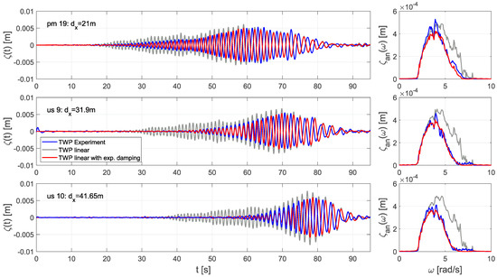
Figure 6.
Comparison between measured vertical displacement of the ice and analytical solution of the linear theory for selected locations. The results in the time domain are shown on the left-hand side and the corresponding amplitude spectra are compared on the right hand side. For linear theory, results for the classical approach as well as for the extended approach by taking the measured damping into account are shown.
5. Discussion
The following is a brief discussion to classify the results shown and to communicate initial experiences with TWP in ice. An important point to keep in mind when using TWPs is the fundamental assumption that the linear theory is applied. This means that the component waves are taken as individual waves which do not interact with each other nor change their wave frequency during propagation in the presence of ice. In contrast to the open water application, this assumption should be reviewed for different scenarios of wave–ice interaction experiments. The occurrence of real-world non-linear effects has been discussed in terms of ice compression, due to wind forcing, [9] as well as wave damping of large amplitude waves [10]. For ice tank applications, we assume that the small amplitude waves used for the generation of the TWP, as well as the short travelling distance under the ice sheet, does not lead to significant non-linear effects.
The model tests showed that experiences from open water experiments cannot be transferred directly to the wave–ice interaction application. The gained experience suggests that both the width of the spectrum and the height of the target wave should be larger. Both ends of the spectrum are very sensitive to measuring errors due to very small initial wave amplitudes. Generally, sensitivity to measuring errors was much more relevant for this test campaign compared to open water experiments as the environmental conditions in terms of low temperature and humidity are more challenging, particularly the permanently changing conditions during the test campaign (i.e., defrosting of the evaporators and subsequent cooling periods), which need to be compensated by the sensors. Defining a wider frequency range shifts this phenomenon outside the relevant frequency range (at least at the beginning of wave propagation). Defining a larger target wave height means that each component wave amplitude within the spectrum is increased, which increases the measurability of the shortest relevant waves within the spectrum. In this context, the selection of the number of sensors and their positions depend on the selected frequency range. The wave attenuation can only be determined if the respective component wave of certain frequency arrives at the next sensor, which is particularly relevant for the shortest waves. In this context, it is worth mentioning that wave attenuation effects, which are not related to the presence of the ice, such as side wall or bottom friction, may be a relevant contribution to the measurement results. To quantify such possible effects, it is straightforward to apply the TWP once in open water in order determine the open water wave attenuation RAO, i.e., wave tank effects. For this study, it is expected that the width of the spectrum was chosen in such a way that significant effects due to side wall and bottom friction can be excluded even for the shortest wave components. However, for shorter waves () or longer wave propagation distances, open water wave attenuation may be observed. Therefore, one should keep in mind that possible wave attenuation is not only related to wave tank effects such as side wall or bottom friction but also to wave energy dissipation.
The general experience of this study is that the TWP concept can be applied to wave–ice interaction experiments. In addition, the presented application showed that the TWP technique enables a very efficient determination of the ice properties in terms of frequency-dependent wave damping over a wide frequency range. For ice tank experiments, it is important to use efficient methods as the time span for experiments is significantly limited compared to open water experiments. On the one hand, preserving the ice properties during the tests requires a sophisticated control system, but the maintenance of constant ice properties over the course of a test day is usually not achieved due to thermal dynamics in the entire tank. On the other hand, the constant bending of the ice due to the waves will lead inevitably to failure at some point. Model ice is more susceptible in this context due to its high plasticity. Thus, TWPs reduce not only the number of experiments significantly, but also allow the investigation of frequency-dependent properties to be carried out under constant conditions (assuming that the ice properties do not change during one short test run). Furthermore, it should be kept in mind that the saved tank time can be used for other research questions. In this context, a TWP could also be used several times over the course of the test campaign to identify possible changes in ice properties.
6. Conclusions
This paper introduced the TWP technique as an efficient method for wave–ice interaction experiments. TWPs are characterised by the fact that all wave components of the spectrum are in phase at a certain so-called concentration point, leading to a single high peak. The main assumption is that the component waves within the spectrum are independent, obeying the linear dispersion relation. For the purpose of this study, the TWP technique was used to generate a tailored synthesised wave group for the investigation of the frequency-dependent wave damping in the presence of an ice sheet. The width of the frequency spectrum, maximum height of the single high wave crest at concentration point and the distance between the concentration point and the wave board can be adjusted to the respective research question. For this study, these parameters were chosen in such a way that the integrity of the ice sheet was ensured. Besides the generation of one TWP, four regular waves with different wave lengths were additionally investigated to evaluate the TWP result.
The general outcome of this study is that TWPs are not only suitable but very efficient for wave–ice interaction investigations. It is shown that the TWP can be used for the investigation of the frequency-dependent wave damping over a wide frequency range. Comparing the results obtained with the TWP and with regular waves revealed a sufficient agreement, as the regular wave results were within the confidence interval of the exponential fit of the TWP attenuation coefficient. The frequency-dependent wave damping coefficient was determined with the TWP measurement, highlighting the significant advantage of this method compared to the classical regular wave approach. The application of the determined frequency-dependent damping coefficient with linear wave theory proved the approach to be in good agreement with the measurements. Further advantages are the existence of an analytical solution as well as the relatively short duration of wave groups. The existence of an analytical solution for the calculation of the wave at the wave board simplifies the method significantly, offering a straightforward plug-and-play solution for test facilities. The short duration of the TWP is not only positive since a large number of test runs in regular waves is avoided, but also due to the fact that the one required test run involves only a few load cycles with regard to ice bending, i.e., the impact on the ice sheet is very small.
However, this application of the TWP concept to wave–ice interaction experiments can be seen as a first step towards establishing the method. Systematic investigation on the applicability of the TWP concept is necessary in order to explore the areas of validity and application.
The following abbreviations are used in this manuscript:
Author Contributions
Conceptualisation: M.K., M.H. and F.v.B.u.P.; methodology: M.K.; software, M.K.; validation: M.K.; formal analysis: M.K., M.H. and F.v.B.u.P.; investigation: M.K., M.H. and F.v.B.u.P.; resources: M.K.; writing—original draft preparation: M.K., M.H. and F.v.B.u.P.; writing—review and editing: M.K., M.H. and F.v.B.u.P.; visualisation, M.K.; supervision: M.K. and F.v.B.u.P.; project administration: M.K.; funding acquisition: M.K. All authors have read and agreed to the published version of the manuscript.
Funding
This paper is published as a contribution to the research project “Nonlinear wave-ice interaction” funded by the Deutsche Forschungsgemeinschaft (DFG, German Research Foundation)—407532845.
Institutional Review Board Statement
Not applicable.
Informed Consent Statement
Not applicable.
Data Availability Statement
Not applicable.
Conflicts of Interest
The authors declare no conflict of interest. The funders had no role in the design of the study; in the collection, analyses, or interpretation of data; in the writing of the manuscript, or in the decision to publish the results.
Appendix A
Figure A1 presents the general overview on the analysis procedure and the results for the tests with regular waves. The two top sub-figures, Figure A1a for the longest investigated regular wave Reg I and Figure A1b for the shortest investigated regular wave Reg IV, illustrate the procedure applied to obtain the statistical quantities of the measured regular waves as an example of one measuring location. The top diagram of each sub-figure presents the measurement as a black curve. For each measurement, an evaluation period was selected by visual inspection. The selection criterion was to ensure that the waves for detailed analysis were not too close to the ramp at the beginning and end of the regular wave train. In addition, the measurements were also evaluated regarding possible influence by wave reflection from the beach, which was only relevant for the last measuring position (seen from the wave board). The selected evaluation period is shown as a blue curve. The bottom diagrams of the two top sub-figures present a close-up view of the selected evaluation period (blue curve). The statistical quantities of the evaluation period were determined by zero-upcrossing analysis, illustrated as a red dashed curve, for which mean wave heights , mean wave periods and the mean crest asymmetries , with for the zero-upcrossing wave crest height, for each regular wave and at each measuring position were obtained.

Figure A1.
Overview on the analysis procedure and measurement results of the investigated regular waves. (a) Example analysis procedure for wave Reg I. The top diagram displays the whole measurement as a black curve and the selected evaluation period as a blue curve. The bottom diagram presents the selected period in detail with the measurement result as a black curve, the selected evaluation period as a blue curve and the identified zero-upcrossing periods for the detailed analysis as a red dashed curve. (b) Example analysis procedure for wave Reg IV. The top diagram displays the whole measurement as a black curve and the selected evaluation period as a blue curve. The bottom diagram presents the selected period in detail with the measurement result as a black curve, the selected evaluation period as a blue curve and the identified zero-upcrossing periods for the detailed analysis as a red dashed curve. (c) Results of the analysis—course of the wave heights (top left), wave periods (top centre) and wave crest asymmetries (top right)—for the four regular waves at each measuring position for the identified evaluation periods. The respective variance of the statistical quantities is illustrated in the bottom diagrams.

Figure A1c presents the results of the detailed analysis for the four investigated regular waves—the course of the wave heights along the ice sheet is presented in the top left, the course of the wave periods in the top centre and the respective wave crest asymmetries in the top right. The course of the wave heights shows the expected characteristic, a decay of the wave amplitude during propagation under the ice sheet with increasing decay rate for decreasing wave periods. The course of the wave periods remains constant over the whole propagation distance. The determined wave crest asymmetry reveals no distinctive difference between wave crest and wave trough, independently of the propagation distance under the ice sheet.
As the presented quantities were determined as the mean value of a certain number of regular waves per measuring position (9 waves for Reg I, 10 waves for Reg II, 14 waves for Reg III and 16 waves for Reg IV), the variance was additionally determined in order to evaluate the regularity of the generated regular waves. For all regular waves as well as quantities, the variance was very small over all measuring locations.
Appendix A
Table A1 presents the important technical details of the applied ultrasonic sensors.
Table A1.
Technical details of the applied us sensors.
Table A1.
Technical details of the applied us sensors.
| Ultralab USS 30250 | Ultralab USS 2001300 | |
|---|---|---|
| Blind area | ||
| Working range | ||
| Techn. resolution | ||
| Reproducibility |
References
- Squire, V.A.; Wadhams, P. Some Wave Attenuation Results from MIZEX-West; CRREL Spec. Rep. 85-06; CRREL: Hanover, NH, USA, 1985.
- Squire, V. Of ocean waves and sea-ice revisited. Cold Reg. Sci. Technol. 2007, 49, 110–133. [Google Scholar] [CrossRef]
- Doble, M.J.; Bidlot, J.R. Wave buoy measurements at the Antarctic sea ice edge compared with an enhanced ECMWF WAM: Progress towards global waves-in-ice modelling. Ocean. Model. 2013, 70, 166–173. [Google Scholar] [CrossRef]
- Montiel, F.; Squire, V.A.; Doble, M.; Thomson, J.; Wadhams, P. Attenuation and Directional Spreading of Ocean Waves During a Storm Event in the Autumn Beaufort Sea Marginal Ice Zone. J. Geophys. Res. Ocean. 2018, 123, 5912–5932. [Google Scholar] [CrossRef]
- Frankenstein, S.; Loset, S.; Shen, H.H. Wave-Ice Interactions in Barents Sea Marginal Ice Zone. J. Cold Reg. Eng. 2001, 15, 91–102. [Google Scholar] [CrossRef]
- Squire, V.A.; Moore, S. Direct measurement of the attenuation of ocean waves by pack ice. Nature 1980, 283, 365–368. [Google Scholar] [CrossRef]
- Wadhams, P.; Squire, V.A.; Goodman, D.J.; Cowan, A.M.; Moore, S.C. The attenuation rates of ocean waves in the marginal ice zone. J. Geophys. Res. Ocean. 1988, 93, 6799–6818. [Google Scholar] [CrossRef]
- Wadhams, P. Ice in the Ocean; CRC Press: Boca Raton, FL, USA, 2000. [Google Scholar]
- Liu, A.K.; Mollo-Christensen, E. Wave Propagation in a Solid Ice Pack. J. Phys. Oceanogr. 1988, 18, 1702–1712. [Google Scholar] [CrossRef]
- Kohout, A.L.; Williams, M.J.M.; Dean, S.M.; Meylan, M.H. Storm-induced sea-ice breakup and the implications for ice extent. Nature 2014, 509, 604–607. [Google Scholar] [CrossRef] [PubMed]
- Liu, A.K.; Vachon, P.W.; Peng, C.Y.; Bhogal, A. Wave attenuation in the marginal ice zone during LIMEX. Atmos. Ocean 1992, 30, 192–206. [Google Scholar] [CrossRef]
- Fox, C.; Haskell, T.G. Ocean wave speed in the Antarctic marginal ice zone. Ann. Glaciol. 2001, 33, 350–354. [Google Scholar] [CrossRef]
- Wadhams, P.; Parmiggiani, F.; de Carolis, G. The Use of SAR to Measure Ocean Wave Dispersion in Frazil-Pancake Icefields. J. Phys. Oceanogr. 2002, 32, 1721–1746. [Google Scholar] [CrossRef]
- Collins, C.O., III; Rogers, W.E.; Marchenko, A.; Babanin, A.V. In situ measurements of an energetic wave event in the Arctic marginal ice zone. Geophys. Res. Lett. 2015, 42, 1863–1870. [Google Scholar] [CrossRef]
- Squire, V.; Allan, A. Propagation of Flexural Gravity Waves in Sea Ice. 1980. Available online: http://hydrologie.org/redbooks/a124/iahs_124_0327.pdf (accessed on 19 March 2021).
- Newyear, K.; Martin, S. A comparison of theory and laboratory measurements of wave propagation and attenuation in grease ice. J. Geophys. Res. Ocean. 1997, 102, 25091–25099. [Google Scholar] [CrossRef]
- Wang, R.; Shen, H.H. Gravity waves propagating into an ice-covered ocean: A viscoelastic model. J. Geophys. Res. Ocean. 2010, 115. [Google Scholar] [CrossRef]
- Zhao, X.; Shen, H.H. Wave propagation in frazil/pancake, pancake, and fragmented ice covers. Cold Reg. Sci. Technol. 2015, 113, 71–80. [Google Scholar] [CrossRef]
- Sutherland, G.; Rabault, J. Observations of wave dispersion and attenuation in landfast ice. J. Geophys. Res. Ocean. 2016, 121, 1984–1997. [Google Scholar] [CrossRef]
- Vance, G. A Scaling System for Vessels Modelled in Ice. In Proceedings of the Society of Naval Architects and Marine Engineers (SNAME) Ice Tech Symposium, Montreal, QC, Canada, 9–11 April 1975. [Google Scholar]
- Schwarz, J. New developments in modeling ice problems. In Proceedings of the 4th International Conference on Port and Ocean Engineering under Arctic Conditions, POAC 77, St. John’s, NB, Canada, 26–30 September 1977; pp. 45–61. [Google Scholar]
- Enkvist, E.; Mäkinen, S. A Fine-Grain Model Ice. In Proceedings of the International Association for Hydro-Environment Engineering and Research (IAHR) on Ice Symposium, Hamburg, Germany, 27–31 August 1984. [Google Scholar]
- Evers, K.; Jochman, P. An Advanced Technique to Improve the Mechanical Properties of Model Ice Developed at the HSVA Ice Tank. In Proceedings of the Conference on Port and Ocean Engineering under Arctic Conditions (POAC), Hamburg, Germany, 17–20 August 1993. [Google Scholar]
- Von Bock und Polach, R. The Mechanical Behavior of Model-Scale Ice: Experiments, Numerical Modeling and Scalability. Ph.D. Thesis, Aalto University, Helsinki, Finnland, 2016. [Google Scholar]
- Von Block und Polach, R.U.F.; Gralher, S.; Ettema, R.; Kellner, L.; Stender, M. The non-linear behavior of aqueous model ice in downward flexure. Cold Reg. Sci. Technol. 2019. [Google Scholar] [CrossRef]
- Von Bock und Polach, R.U.F. Numerical analysis of the bending strength of model-scale ice. Cold Reg. Sci. Technol. 2015, 118, 91–104. [Google Scholar] [CrossRef]
- von Bock Und Polach, R.U.F.; Ziemer, G.; Klein, M.; Hartmann, M.C.N.; Toffoli, A.; Monty, J. Case based scaling: Recent developments in ice model testing technology. In Proceedings of the International Conference on Offshore Mechanics and Arctic Engineering—OMAE: Virtual Conference, Online, 3–7 August 2020; Volume 7. [Google Scholar] [CrossRef]
- Squire, V.A. A theoretical, laboratory, and field study of ice-coupled waves. J. Geophys. Res. Ocean. 1984, 89, 8069–8079. [Google Scholar] [CrossRef]
- Shen, H.H.; Ackley, S.F.; Yuan, Y. Limiting diameter of pancake ice. J. Geophys. Res. Ocean. 2004, 109. [Google Scholar] [CrossRef]
- Cheng, S.; Tsarau, A.; Li, H.; Herman, A.; Evers, K.U.; Shen, H. Loads on Structure and Waves in Ice (LS-WICE) Project, Part 1: Wave Attenuation and Dispersion in Broken Ice Fields. In Proceedings of the 24th International Conference on Port and Ocean Engineering under Arctic Conditions (POAC 2017), Busan, Korea, 11–16 June 2017. [Google Scholar]
- Herman, A.; Tsarau, A.; Evers, K.U.; Li, H.; Shen, H. Loads on Structure and Waves in Ice (LS-WICE) Project, Part 2: Sea Ice Breaking by Waves. In Proceedings of the 24th International Conference on Port and Ocean Engineering under Arctic Conditions (POAC 2017), Busan, Korea, 11–16 June 2017. [Google Scholar]
- Rabault, J.; Sutherland, G.; Jensen, A.; Christensen, K.; Marchenko, A. Experiments on wave propagation in grease ice: Combined wave gauges and particle image velocimetry measurements. J. Fluid Mech. 2019, 864, 876–898. [Google Scholar] [CrossRef]
- Yu, J.; Rogers, W.E.; Wang, D.W. A Scaling for Wave Dispersion Relationships in Ice-Covered Waters. J. Geophys. Res. Ocean. 2019, 124, 8429–8438. [Google Scholar] [CrossRef]
- Marchenko, A.; Haase, A.; Jensen, A.; Lishman, B.; Rabault, J.; Evers, K.; Shortt, M.; Thiel, T. Elasticity and viscosity of ice measured in the experiment on wave propagation below the ice in HSVA ice tank. In Proceedings of the 25th IAHR International Symposium on Ice; The International Association for Hydro-Environment Engineering and Research (IAHR): Virtual Conference, Online, 23–25 November 2020. [Google Scholar]
- Damping of Regular Waves in Model Ice, Volume 7: Polar and Arctic Sciences and Technology. Int. Conf. Offshore Mech. Arct. Eng. 2020. [CrossRef]
- Marchenko, A.; Haase, A.; Jensen, A.; Lishman, B.; Rabault, J.; Evers, K.; Shortt, M.; Thiel, T. Laboratory Investigations of the Bending Rheology of Floating Saline Ice and Physical Mechanisms of Wave Damping In the HSVA Hamburg Ship Model Basin Ice Tank. Water 2021, 13, 1080. [Google Scholar] [CrossRef]
- Clauss, G.F.; Bergmann, J. Gaussian wave packets – a new approach to seakeeping tests of ocean structures. Appl. Ocean. Res. 1986, 8, 190–206. [Google Scholar] [CrossRef]
- Clauss, G.; Kühnlein, W. Seakeeping Tests in Transient Wave Packets. In Proceedings of the International Conference on Offshore Mechanics and Arctic Engineering, Kopenhagen, Denmark, 18–22 June 1995. [Google Scholar]
- Clauss, G.; Kühnlein, W. A new tool for seakeeping tests—Nonlinear transient wave packets. In Proceedings of the 8th International Conference on the Behaviour of Offshore Structures (BOSS), Delft, The Netherlands, 7–10 July 1997; pp. 269–285. [Google Scholar]
- Davis, M. Testing ship models in transient waves. In Proceedings of the 5th Symposium on Naval Hydrodynamics, Bergen, Norway, 10–12 September 1964. [Google Scholar]
- Takezawa, S.; Hirayama, T. Advanced experimental techniques for test-ing ship models in transient water waves. Part II: The controlled transientwater waves for using in ship motion tests. In Proceedings of the 11th Symposium on Naval Hy-drodynamics: Unsteady Hydrodynamics of Marine Vehicles, London, UK, 28 March–2 April 1976. [Google Scholar]
- Mansard, E.; Funke, E. A new approach to transient wave generation. Coast. Eng. Proc. 1982, 1, 45. [Google Scholar] [CrossRef]
- Grigoropoulos, G.; Florios, N.; Loukakis, T. Transient waves for ship and floating structure testing. Appl. Ocean. Res. 1994, 16, 71–85. [Google Scholar] [CrossRef]
- Airy, G. Tides and Waves. Encycl. Metrop. 1845, 3, 241–396. [Google Scholar]
- Newman, J. Marine Hydrodynamics; The MIT Press: Cambridge, MA, USA, 1977. [Google Scholar]
- Mei, C. The Applied Dynamics of Ocean Surface Waves; Wiley: Hoboken, NJ, USA, 1983. [Google Scholar]
- Chakrabarti, S.K. Hydrodynamics of Offshore Structures; Springer: Berlin/Heidelberg, Germany, 1987; ISBN 3-540-17319-6. [Google Scholar]
- Clauss, G.; Lehmann, E.; Östergaard, C. Offshore Structures; Conceptual Design and Hydrodynamics; Springer: London, UK, 1992; Volume 1. [Google Scholar]
- Fox, C.; Squire, V.A. On the oblique reflexion and transmission of ocean waves at shore fast sea ice. Philos. Trans. R. Soc. London. Ser. A Phys. Eng. Sci. 1994, 347, 185–218. [Google Scholar] [CrossRef]
- Rabault, J. An Investigation into the Interaction between Waves and Ice. Ph.D. Thesis, University of Oslo, Oslo, Norway, 2018. [Google Scholar]
- Clauss, G.F.; Steinhagen, U. Numerical simulation of nonlinear transient waves and its validation by Laboratory data. In Proceedings of the 9th International Offshore and Polar Engineering Conference (ISOPE), Brest, France, 30 May–4 June 1999; Volume III, pp. 368–375. [Google Scholar]
- Kühnlein, W.L.; Clauss, G.F.; Hennig, J. Tailor made freak waves within irregular seas. In Proceedings of the International Conference on Offshore Mechanics and Arctic Engineering, Oslo, Norway, 23–28 June 2002; Volume 36142, pp. 759–768. [Google Scholar]
- Clauss, G.F.; Klein, M.; Dudek, M. Influence of the Bow Shape on Loads in High and Steep Waves. In Proceedings of the International Conference on Ocean, Offshore and Arctic Engineering, Shanghai, China, 6–11 June 2010. [Google Scholar] [CrossRef]
- Hennig, J. Generation and Analysis of Harsh Wave Environments. Doctoral Thesis, Technische University, Berlin, Germany, 2005. [Google Scholar]
- Clauss, G.F.; Stuppe, S.; Dudek, M. Transient Wave Packets: New Application in CFD-Methods, Volume 8B: Ocean Engineering. In Proceedings of the ASME 2014 33rd International Conference on Ocean, Offshore and Arctic Engineering, San Francisco, CA, USA, 8–13 June 2014. [Google Scholar] [CrossRef]
- ITTC. Ice Property Measurements, 7.5-02-04-02; ITTC: Zürich Switzerland, 2014. [Google Scholar]
- Von Bock und Polach, R.U.F.; Molyneux, D. Model ice: A review of its capacity and identification of knowledge gaps. In Proceedings of the ASME 2017 36st International Conference on Ocean, Offshore and Arctic Engineering, Trondheim, Norway, 25–30 June 2017; p. 9. [Google Scholar]
- Zufelt, J.E.; Ettema, R. Model Ice Properties; Technical Report CRREL Report 96-1; U.S. Army Corps of Engineers; Cold Regions Research and Engineering Laboratory (CRREL): Hanover, NH, USA, 1996.


Publisher’s Note: MDPI stays neutral with regard to jurisdictional claims in published maps and institutional affiliations. |
© 2021 by the authors. Licensee MDPI, Basel, Switzerland. This article is an open access article distributed under the terms and conditions of the Creative Commons Attribution (CC BY) license (https://creativecommons.org/licenses/by/4.0/).