Article

How Well Can Machine Learning Models Perform without Hydrologists? Application of Rational Feature Selection to Improve Hydrological Forecasting

by
Vsevolod Moreido
1,
Boris Gartsman
1,
Dimitri P. Solomatine
1,2,3,* and
Zoya Suchilina
1
1
Water Problems Institute, Russian Academy of Sciences, 11333 Moscow, Russia
2
Hydroinformatics Chair Group, IHE Delft Institute for Water Education, 2611 AX Delft, The Netherlands
3
Water Resources Section, Delft University of Technology, 2628 CD Delft, The Netherlands
*
Author to whom correspondence should be addressed.
Water 2021, 13(12), 1696; https://doi.org/10.3390/w13121696
Submission received: 2 May 2021 / Revised: 3 June 2021 / Accepted: 10 June 2021 / Published: 19 June 2021

Abstract

:
With more machine learning methods being involved in social and environmental research activities, we are addressing the role of available information for model training in model performance. We tested the abilities of several machine learning models for short-term hydrological forecasting by inferring linkages with all available predictors or only with those pre-selected by a hydrologist. The models used in this study were multivariate linear regression, the M5 model tree, multilayer perceptron (MLP) artificial neural network, and the long short-term memory (LSTM) model. We used two river catchments in contrasting runoff generation conditions to try to infer the ability of different model structures to automatically select the best predictor set from all those available in the dataset and compared models’ performance with that of a model operating on predictors prescribed by a hydrologist. Additionally, we tested how shuffling of the initial dataset improved model performance. We can conclude that in rainfall-driven catchments, the models performed generally better on a dataset prescribed by a hydrologist, while in mixed-snowmelt and baseflow-driven catchments, the automatic selection of predictors was preferable.

1. Introduction

To date, hydrological modelling has proven to be a reliable solution for a plethora of tasks, both research and applied, such as water resources planning, flood hazard analysis, civil engineering, structure design, operational forecasting, impact analysis, land–atmosphere interaction analysis, cold season processes, and ecohydrology [1,2,3]. For more than 70 years, the hydrological community has been developing a variety of model designs for the aforementioned applications, from simple data-driven mechanistic models (referred to as ‘black boxes’) to complex spatially distributed process-based models [2]. The detail of the complexity of a model largely depends on the specific application it is aimed for, e.g., for hydrological forecasting, a complex process-based spatially distributed model might be redundant [4,5], while for an impact assessment study, detailed information on watershed states and fluxes is crucial [2] and can only be provided by a complex model based on a detailed description of physics.
In the last 30 years, a new class of data-driven models, namely, machine learning (ML) models, has emerged (e.g., [6,7,8]). With their development, ML models and artificial neural network (ANN) models, in particular, have shown capabilities to solve various applied tasks while bypassing the problems of weak representation of hydrological processes and lack of detailed regional catchment information to apply complex process-based models [4]. However, ML models are also criticized, mainly for their poor interpretability [6]. There have been researching efforts aimed at inferring a hydrologically relevant model structure from the ML model, either based on internal states of a neural network [5,9,10,11] or feature importance analysis [12]. An emerging trend is to incorporate physics directly into the learning process (see e.g., [13]). All these years there exists an ongoing discussion regarding the applicability of such models to tasks where the system insight is sought (e.g., [4]).
Nevertheless, the ML models have proven to be capable of solving hydrological forecasting tasks [6,12,14,15] by an effective utilization of linear linkages between multiple predictor variables (features) and hydrological variables, such as, but not limited to, streamflow runoff (target). Recent developments in ML, in particular, deep learning (DL) models (mainly, recurrent networks), have led to yet another wave of interest in ML models [5,11,16]. This interest is based on reports that in many disciplines, other than hydrology, employing DL, such models have shown new advanced capabilities of discovering and utilizing nonlinear linkages between features and targets. The abilities of DL models to outperform conceptual hydrological models in forecasting streamflow in ungauged basins has started a discussion on the conceptual models’ fate in the future world [4,5,17]. However, the main requirement of such models is a sufficient amount of quality data to train and validate the model, and several major issues are worth mentioning here.
Despite the rapid development of novel Earth observation systems and technologies, in many parts of the world, the existing monitoring networks operate with traditional routines of atmosphere and river system measurements, yielding a set of monitoring variables of low spatial and temporal resolution. Hence, forecasters are frequently left with only limited data available. However, as the name implies, rainfall–runoff modelling has developed several concepts for making forecasts using basic data on precipitation and runoff measurements, such as employing time series (auto)correlation, residence time, basin storage, and so on [18,19]. Although ML models can help to discover new connections between the observations and the output, their application in the aforementioned regions, or ungauged basins, might run into a significant lack of data, which would prevent an effective performance. The length of time series might also be a limitation, especially for multilayer DL models with a very high number of parameters to train, as such networks are most effective with big data [11].
The existing requirement for a model dataset to be split for training and validation subsets having similar statistical distributions [20] also might reduce the input time series for effective model fitting. Yet another issue from a technical side is that, even when having a sufficient amount of data, an exhaustive search for the best set of the input lagged variables can be computationally expensive, as n predictors over k lags yield (2n − 1)k possible combinations [15]. Refitting such a model on new data requires a significant amount of time and modern hardware.
All these considerations have prompted researchers to use an additional step in building ML models, often called input variables selection (IVS; see, e.g., [21]). Its purpose is to apply data analysis to discover correlations between various (lagged) variables and the output or, using metrics based on mutual information, to select an optimal (candidate) set of inputs before a model is built.
The main objective of this paper is to explore several strategies to construct candidate sets of inputs for several types of ML models, ranging from their automatic selection to the direct use of hydrological knowledge about the modeled catchment. With this, we hope to contribute to the current discussion on the usefulness of using hydrological knowledge in building ML models.
Given the aforementioned advantages and limitations of the ML models and previously conducted research, we have conceived this paper so to discuss and answer the following research questions:
  • Can rational (e.g., manual, based on empirical knowledge) feature selection improve the performance of an ML model of future streamflow runoff, compared to models with automatically selected features?
  • Can this effect be retained in different ML model types and structures, including the DL model?
  • Can the stochastic shuffling of input streamflow runoff time series for building training and test sets improve the overall model accuracy?
For this discussion, we employed several ML models, namely, multivariate linear regression (LM), M5 model tree [22], multilayer perceptron (MLP), and long short-term memory (LSTM) model for two case study catchments in contrasting climate conditions. A description of the case study catchments is given in Section 1. Models’ structures are described in Section 3. Methods for feature selection are introduced in Section 3. The obtained results are discussed in Section 4, and conclusions are presented in the last section.

2. Materials and Methods

2.1. Case Study Catchments

Two case studies were selected for the assessment, significantly different in basin size, natural conditions, and hydrological regime.
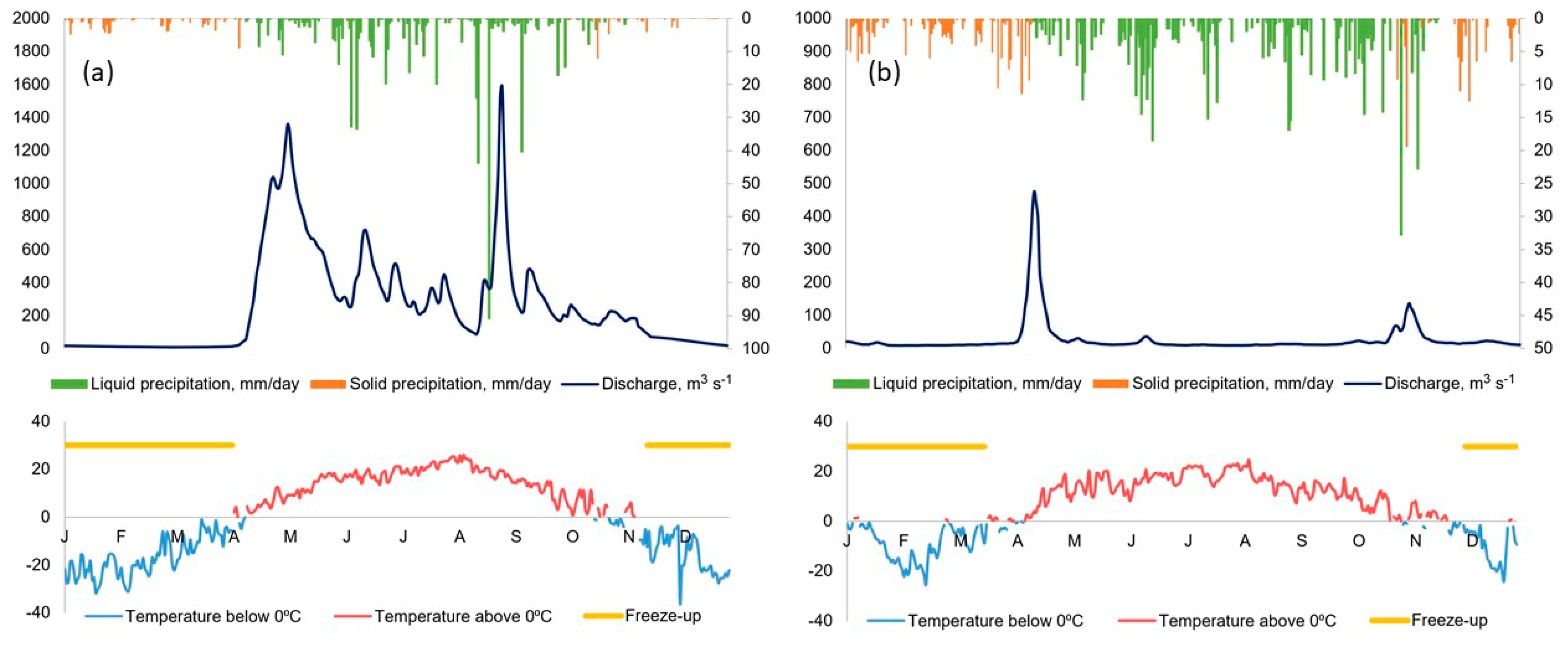
The Ussuri River catchment is situated in the southern part of the Far East of Russia (Figure 1) within the Amur River basin. The river is 897 km long, the basin area is 193,000 km2. The climate of the region is highly influenced by its location near the Pacific Ocean and by monsoon circulation. The precipitation is highly variable both intra- and interannually. Typical for the catchment region is a warm damp summertime and a cold dry wintertime. The mean air temperature in August is +21 °C, and in January it is −20 °C. In the mountainous part of the catchment, the precipitation amount reaches 1000 mm annually, while in the lower part, it reaches around 600 mm, mostly (70%) occurring in summer and fall. From July to September, the region is influenced by tropical cyclones (typhoons), leading to river flooding and floodplains’ inundation. Around 20% of the precipitation falls as snow. Snow cover lasts for 140–210 days annually in the mountainous part, and for 85–140 days annually in the lower part of the catchment. The river regime is typical for the Far East and is characterized by frequent floods; around 80% of the runoff is generated by rainfall. The spring freshet is relatively low, with most of the runoff (95%) occurring in summer and fall. Winter low flows account for 2–5% of the annual runoff.
The second case study—the Protva river—is a small river catchment, third-order tributary to the Volga river (Figure 1). The river is 282 km long, and the basin area is 4620 km2. The catchment is located in a moderate climate with a cold wintertime and a moderately warm summer, with frequent rainstorms determining the weather in both periods. Up to 90% of precipitation occurs during cyclones. The water regime is of Eastern European type, with the spring freshet prevailing over other seasons. In summer and fall, relatively small storm flooding occurs. The catchment size determines its sensitivity to shower rains in the summertime and to thawing in the wintertime. The runoff is dominantly snowmelt-fed (50%), with active ground storage (30%) and direct rain-fed stormflow (20%, see Figure 2).

2.2. ML Models

Several model designs were built to perform tests at each catchment: LM—a multivariate linear regression model with least-squares optimization—M5P—a modified decision tree model with linear regression models at the nodes [22], which acts as a piecewise linear model—multilayer perceptron (MLP)—an artificial neural network with nonlinear activation function in neurons [23]—and finally the long short-term memory model (LSTM)—a deep learning neural network with several state variables [24]. All models were built in Python environment as jupyter notebook documents using the open-source machine learning libraries scikit-learn [25] and Weka [26].

2.3. Initial Data Description

The initial datasets for both catchments were based on standard weather and streamflow observations by the monitoring network maintained by the Russian Hydrometeorological Service. In this respect, the data are equivalent to those available in streamflow forecasters’ daily routine.
The dataset for the Ussuri River at Kirovsky gauging station, controlling an area of 24,400 km2, consists of daily time series of air temperature and precipitation amount at 3 weather stations and daily streamflow discharge at the basin outlet (Figure 1) for the period 1979–1986.
For the Protva River at the Spas-Zagorie gauging station, controlling an area of 3640 km2, a similar dataset was created: time series of daily temperature and precipitation at 3 weather stations and streamflow discharge at the basin outlet (Figure 1) for the period 2003–2015.
Modeling of streamflow discharges for both rivers was carried out only for the warm period of the year—from 16 May to 31 October—to include the period of rainfall-induced runoff and neglect the runoff due to snowmelt. Every day within the time series period, a 7 day ahead forecast was computed using all previously available data. The datasets included a time series of 58 predictors derived from the initial data, as well as a 7 day ahead streamflow discharge time series as predictands. The datasets included (Table 1):
  • Streamflow discharge at the basin outlet at current day and 7 days before Q t τ , τ = 1, …, 7;
  • Maximum streamflow discharge spread in the preceding period of 2 to 7 days Δ Q m a x τ , τ = 2, …, 7;
  • Daily precipitation amount at individual weather stations for each day in the preceding 7 day period P t τ ;
  • Basin-averaged daily precipitation amount for each day in the preceding 7 day period P ¯ t τ ;
  • Accumulated precipitation for the preceding period of 2 to 7 days P t τ ;
  • Accumulated daily temperatures from the beginning of the warm period above three thresholds 0, +2 и +5 °С T ;
  • Preceding moisture content index I W [27], calculated from the basin-averaged precipitation of the preceding 60 days as
    I W = P t + 0.7 τ = 1 4 P t τ + 0.5 τ = 5 9 P t τ + 0.3 τ = 10 14 P t τ + 0.2 τ = 15 30 P t τ + 0.1 τ = 31 60 P t τ ,
  • Accumulated potential evaporation from the beginning of the warm period, calculated as [28]:
    P E T = {   0.408 R e ( T + 5 ) 100 ,   п р и   T + 5 > 0 0
    where P E T   is the daily potential evaporation amount, in mm, Re it the incoming solar irradiance, in W, T is the mean daily air temperature, in °С.
The input dataset structure details are presented in Table 1. All predictands (future streamflow discharges for subsequent days, referred to as targets) and predictors (features) are arranged in the dataset column-wise, preceded by the daily timestamp. The past streamflow, its spread, and precipitation are referred to as “dynamic” predictors, describing frequent changes in the initial forecasting conditions. The remaining features are referred to as “inertial”, accumulating the basin information for a certain time (60 days at most). Hence, each row of the created dataset represents an encapsulated data structure, holding basin-wide features and targets for each timestep. The full length of the datasets totaled 1352 timesteps for the Ussuri and 2197 timesteps for the Protva river.
The “dynamic” features represent the current and past information (with lag up to 7 days); the forecast was also issued for lead times up to 7 days. This time scale was selected to provide the model with previous basin information from the lag time not less than from the lead time. The timescale was inferred from the manual assessment of hydrographs and hyetographs in both catchments, as well as from the (auto)correlation analysis of the features’ and targets’ (lagged) time series. The correlation between the lagged observed daily precipitation at the individual weather stations and streamflow runoff at the basin outlet for the Ussuri River basin at best never exceeded 0.2, and that for the Protva River basin never exceeded 0.17. This showed that in the Ussuri catchment, the concentration time was 4–5 days, while in the Protva catchment, it was 3–4 days. Hence, we assumed the selected lag time included the timescale of any rain flood event in both catchments.
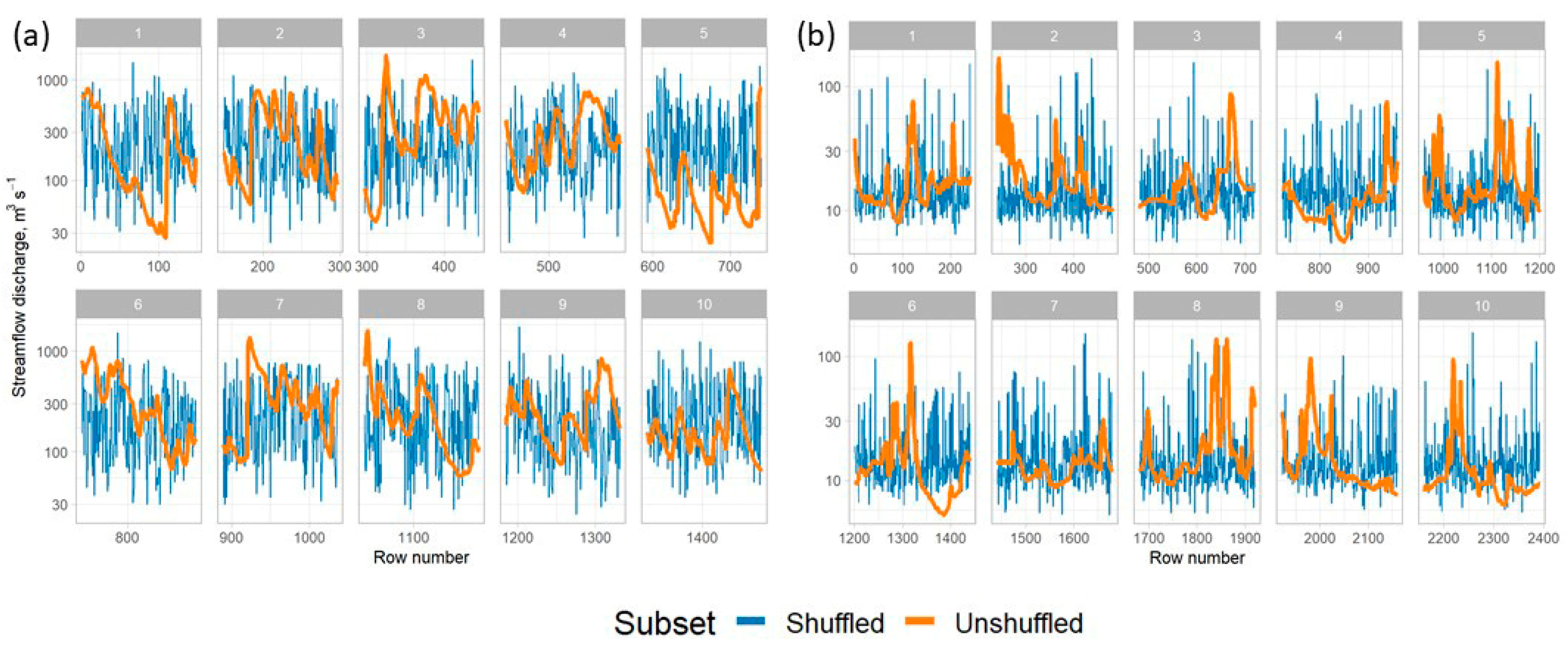
According to the generally accepted procedures of building machine learning models (e.g., [20]), it is recommended to divide the dataset into a training and a test set (and, ideally, also into a cross-validation set) of appropriate size with similar probability distribution. Due to the stochastic nature of streamflow, the latter requirement seems elusive when dividing the initial time series, especially when the k-fold cross-validation is used for the model hyperparameter optimization. We addressed this issue by random shuffling of the initial dataset, thus greatly reducing the variability between the dataset subsamples (Figure 3). The coefficient of variation of the mean values of 10 subsamples of the shuffled dataset for the Ussuri river was 74% lower than that of the unshuffled one, i.e., 0.09 with respect to 0.36. For the Protva River, random shuffling showed similar results: reduction of the coefficient of variation by 72% from 0.20 to 0.05 for the shuffled with respect to the unshuffled. The aforementioned design of the dataset where each row represents several “dynamic” and “inertial” features allowed for such random shuffling, thus keeping the statistical interrelations between the data intact. The resulting datasets were divided into two subsets: 80% of the data for training and 20% for testing.
The mentioned random shuffling was not applied to the dataset for the LSTM model, because this model requires a different (yet similar) data preparation procedure [29]. For each set of the predictands Q t + τ , a subset of lagged predictors was formed, with a lag of 60 days to keep it consistent with the randomly shuffled dataset. Afterwards, the batches were shuffled and randomly fed into the model for training and testing.

2.4. Feature Selection and Experimental Design

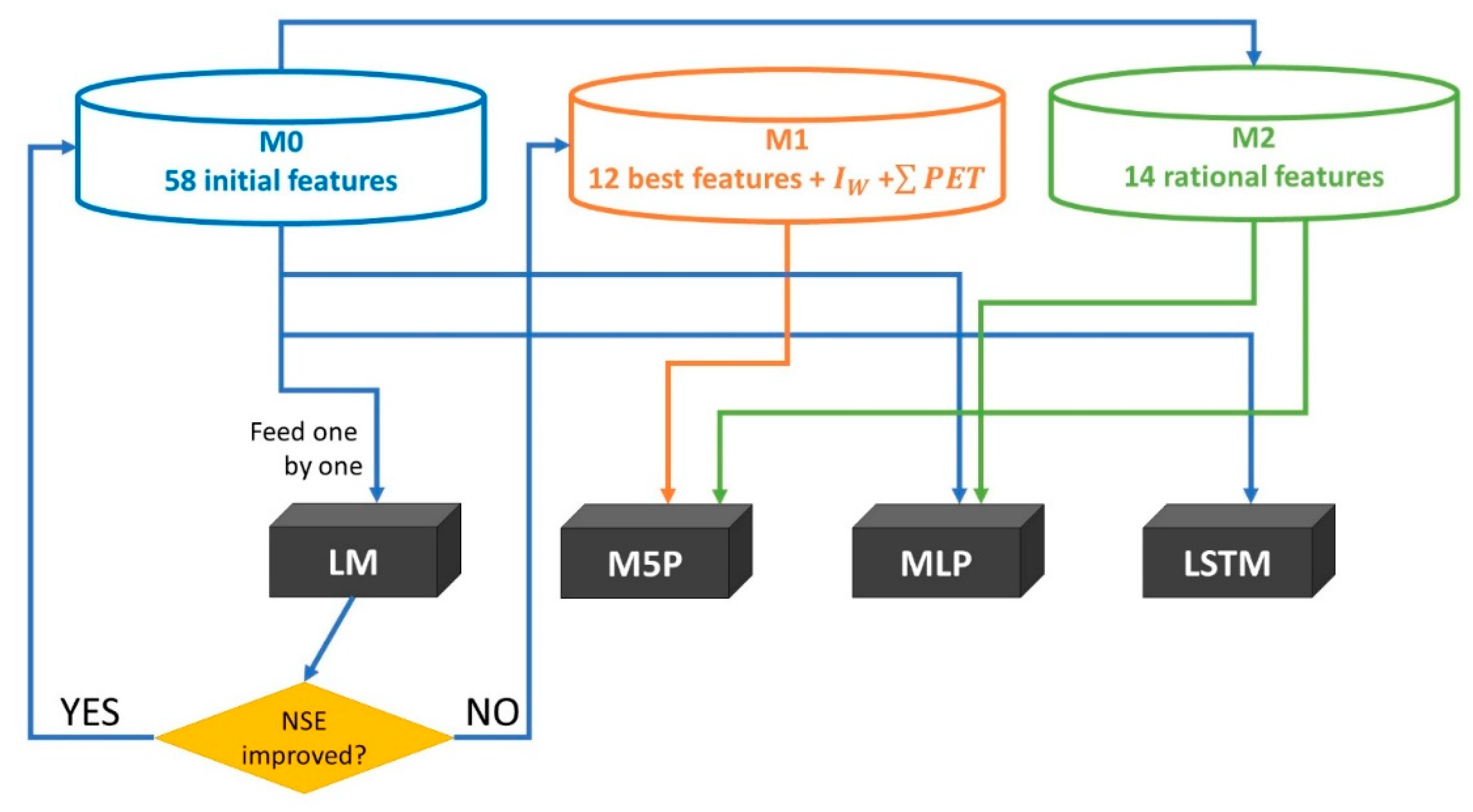
To select the most effective features from the initial set, we used the following methodology. First, we used “greedy selection”, gradually adding features from the initial set to the linear model (LM) to predict streamflow discharges 1 to 7 days ahead until the evaluation metric on the test dataset ceased to increase. Eventually, for each lead time, we obtained 19 efficiency-ranked sets of features, some of which were repeated. Of those, we calculated weighted ranks overall lead times to select 12 top-ranked features. Those 12 features, plus two “inertial” features ( I W and P E T ), formed the feature set, hereafter referred to as M1 (Figure 4, Table 2).
Next, we used what we call in this paper rational feature selection, an expert-based approach to feature set construction relying upon the physical characteristics of the rainfall–runoff processes in the selected catchments. This set comprised (Table 2): streamflow discharge at the catchment outlet (Qt−τ), maximum discharge spread ( Δ Q m a x ), basin-averaged precipitation amount ( P ¯ t τ ), accumulated precipitation ( P ) or accumulated daily temperatures ( T ), preceding moisture content ( I W ), and accumulated potential evaporation ( P E T ). The feature sets for both rivers were generally similar, except that the accumulated temperatures were selected only for the Protva river, and the accumulated precipitation only for the Ussuri river; the lags used for averaged precipitation were also different.
All the conducted experiments are shown in Table 3. We used LM with M0 feature set as a reference for all other models and sets. The piecewise linear regression model M5P and MLP ANN were fed with the M1 and M2 sets, and LSTM was fed with the full M0 set.

2.5. Model Training and Testing Methodology

We employed the following, quite traditional, model performance and error metrics. To assess the mean error, we used the root-mean-squared error estimation calculated as
R M S E = 1 N i = 1 N ( Q i p Q i o ) 2 ,
where Q i p is the streamflow value predicted at lead time τ (m3 s−1), Q i o is the observed value (m3 s−1), N is the length of the training or test sample.
To assess the model efficiency, we calculated the Nash–Suttcliffe criterion as
N S E = 1 i = 1 N ( Q i p Q i o ) 2 i = 1 N ( Q i o Q o ¯ ) 2 .
To assess the forecasts’ efficiency against the persistence forecast, we used a normalized error skill score, common to operational forecasts’ verification in Russia (Borsch and Simonov, 2016), also referred to as “Inertial R M S E ” or I R M S E [30], calculated as
I R M S E = R M S E σ Δ ,  
where
σ Δ = 1 N i = 1 N ( Δ i Δ ¯ ) 2 ,  
Δ i = Q i o Q i + τ o ,   τ = 1 ,   ,   7 ,  
Δ ¯ = 1 N i = 1 N Δ i
R M S E is the mean-squared-error of the forecast as in (2), σ Δ is the error of the persistence forecast over each lead time, calculated as the standard deviation of the lagged observed time series, Δ i . The range of I R M S E values is 0 to +∞, the best value is 0. I R M S E values ranging between 0 and 0.5 are considered a good forecast, from 0.5 to 0.7 are considered fair, from 0.7 to 1.0, poor, above 1, useless [31].

3. Results

Model Performance Evaluation

We believe the performance assessment of individual models on all lead times between the two contrasting catchments provided a certain insight on the feature importance and model structure.
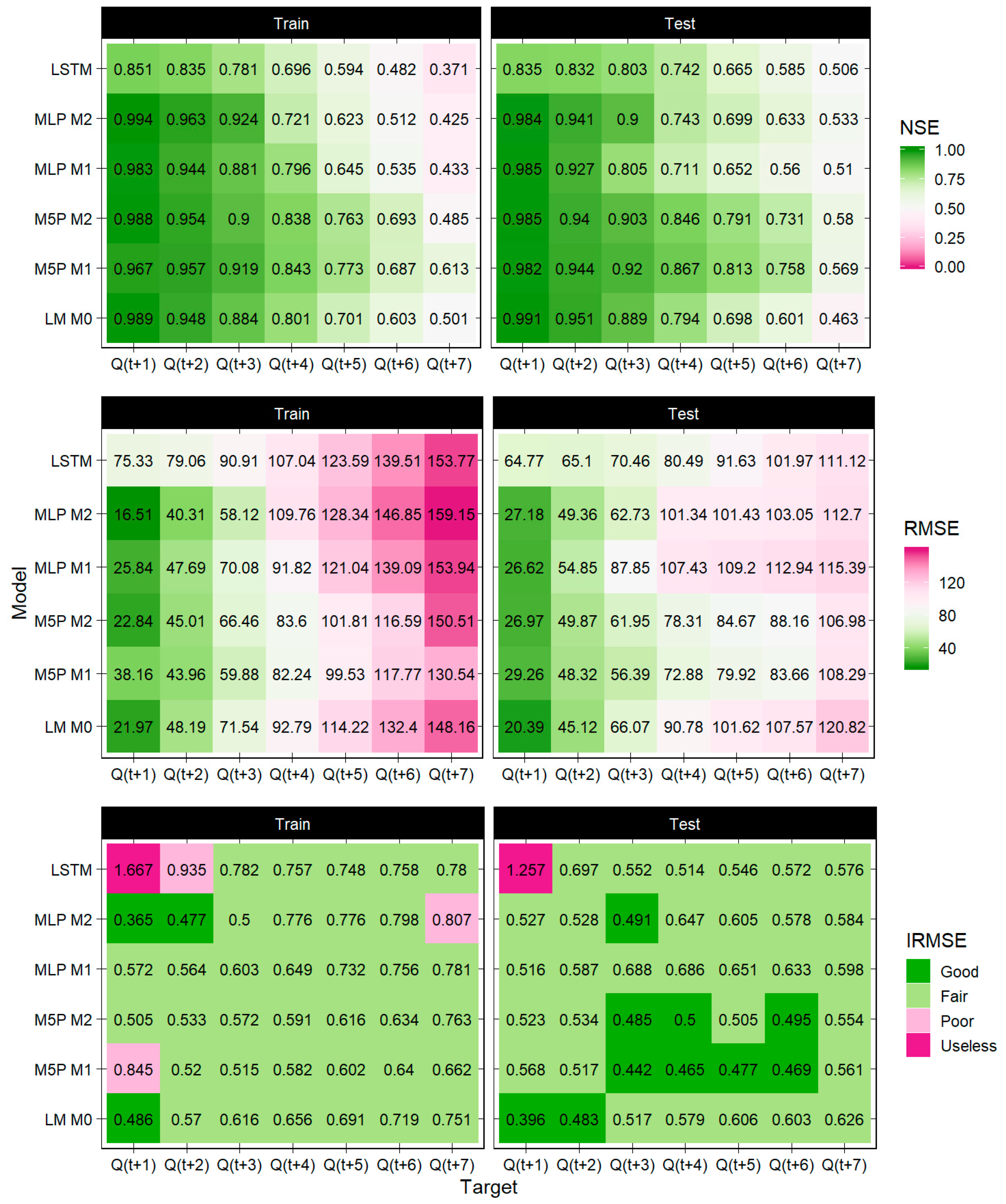
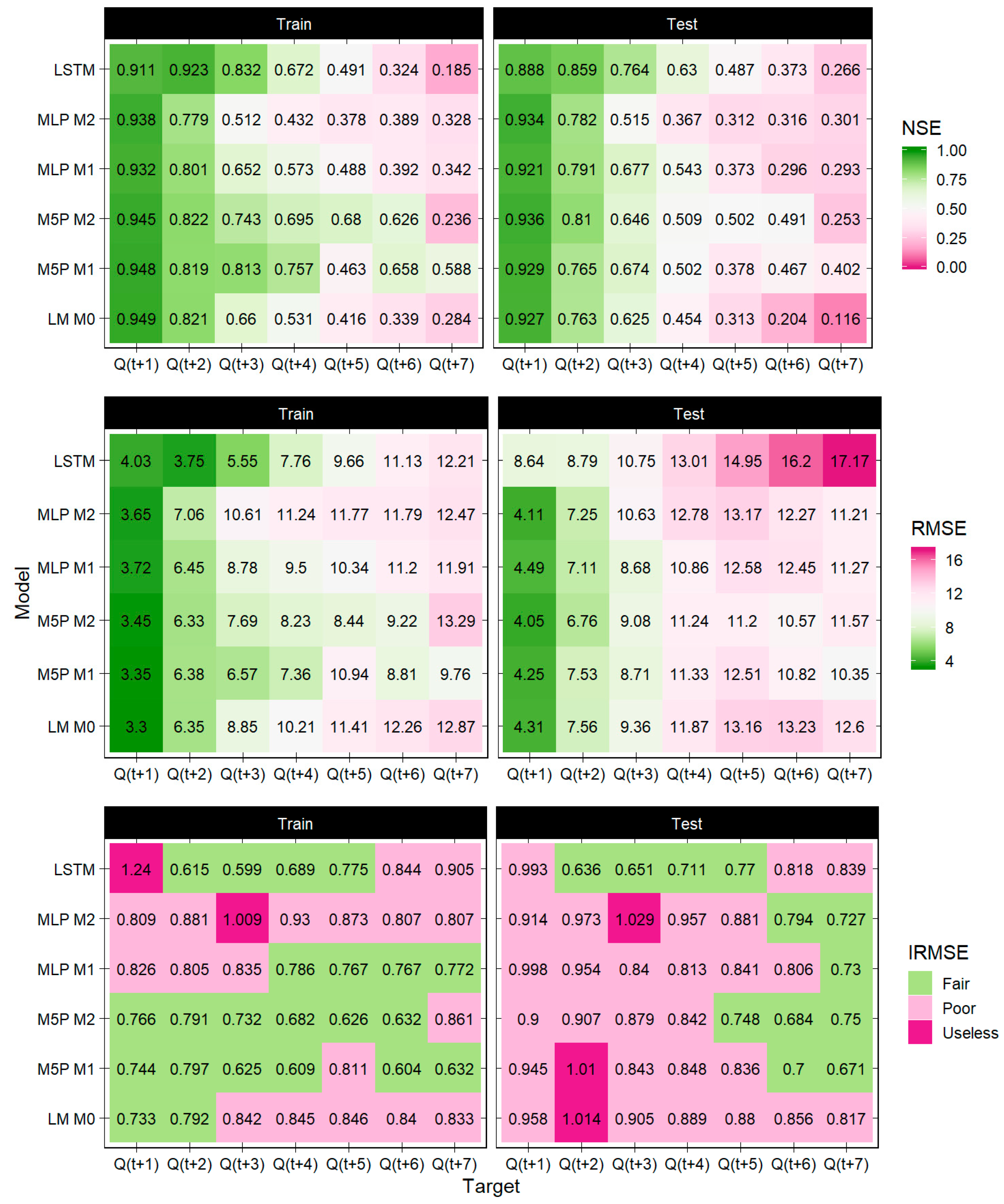
For the Ussuri basin (Figure 5), all models showed good performance both on training and test datasets. NSE values were close to 1 on small lead times and remained above the “predictability threshold”, defined as 1/е ≈ 0.37, for quadratic performance metrics [32]. However, the LSTM showed relatively poorer results on the first lead time as compared to other models, performing close to the MLP models. For the one-day ahead lead-time, the LM and MLP M2 models performed best in terms of all metrics. Considering all metrics on all lead times, the M5P models showed the best performance, retaining “good” forecasts on the test set in terms of the IRMSE values on lead times 3 through 6. Between the models, the MLP M1 model in this particular catchment showed the best results. The second-best model, showing similar results, was the M5P M2 model with “rational” features. For the Ussuri catchment, the models’ performance generally deteriorated as their complexity increased. For one-day lead-time, the LM model was the best, for lead times 2 through 7, the (piecewise linear) M5P models were the best. On the test sample, the models performed slightly better, and this, we believe, shows the advantage of sample shuffling to include a wider distribution of cases for model training as compared to (non-shuffled) time series.
For the Protva catchment, the models’ performance was significantly different (Figure 6). The results were generally much poorer than those for the Ussuri catchment, the models’ efficiency deteriorated more rapidly and fell beyond the “predictability threshold” on the 5 day lead time. Based on the IRMSE values, no model can be considered “good”; however, the LSTM performed fairly on lead times 2 to 5 on both training and test samples, and the M5P M2 and M5P M1 results were mostly fair on the training sample and turned fair on lead times 5 to 7 on the test sample. There was little agreement between the metrics, yet on the test sample, the M5P M2 showed generally better results in terms of NSE and RMSE, but not IRMSE. LSTM showed good retaining capability up to lead time 5 but was outperformed by the M5P.
Another observation concerns the performance of the MLP model with the two feature sets on the two catchments. For the Ussuri river, the MLP M2 with a limited feature set performed slightly better than the MLP M2; the opposite was observed for the Protva River.

4. Discussion and Conclusions

The assessed models’ performance on the two contrasting catchments led to several concluding statements:
  • Overall, the models’ performance for the selected period of rainfall floods was better and more stable for the Ussuri river catchment than for the Protva river catchment;
  • Deterioration of forecasting accuracy was more rapid and pronounced for Protva than for Ussuri; the “predictability threshold” was reached in 5 days of lead time for Protva, yet extended to more than 7 days for Ussuri;
  • For both catchments, the LM and (piece-wise linear) M5P models outperformed ANNs on all lead times; however, the LSTM model was also effective on both training and test samples;
  • For Ussuri, the performance of M5P M1 and M5P M2 was similar, yet this was not observed for Protva;
  • The MLP M1 and MLP M2 models showed contrasting results for different catchments, with the MLP M2 performing better than the MLP M1 for Ussuri, while the opposite was observed for Protva.
The discovered differences in the models’ performance in different catchments can be explained considering the different natural conditions. For the Ussuri catchment, the flood season annually prevails, with frequent and intensive cyclone- or typhoon-induced rainfall, simultaneously affecting vast territories of the catchment. Given the catchment mountainous setting and thin quaternary cover, this leads to fast catchment damping and overland flow. This rainfall–runoff pattern is underpinned by the high values of the rain floods runoff coefficient, which are above 0.7.
The prevailing season in the Protva catchment is spring freshet, while rain floods in the summer and fall are much less pronounced. They are formed by frontal and airmass-associated rainstorms that occur unevenly over the catchment (despite its small size), which can be seen in the low correlation between the rainfall and the runoff. Unpronounced surface elevation and thick quaternary cover determine the slow catchment response to rainfall, greater loss of precipitated water, and nonlinearity of runoff generation processes, which is demonstrated by the low values of the runoff coefficient for rain floods, which is below 0.5. One manifestation of this nonlinearity can be seen in the controversial results of the MLP M1 and M2 models for Protva, where the reduction of features by their rational selection did not necessarily improve the models’ performance, yet a nonlinear model could perform better.
Thus, regardless of the larger Ussuri catchment size compared to Protva and the longer concentration time, the Ussuri catchment can be seen as a much more integrated basin in terms of response to external forcing. Rainfall–runoff transformation in the Ussuri catchment is more rapid and synchronous than in the Protva catchment, and hence can be better described by simpler piece-wise linear models. On the contrary, the Protva catchment is more heterogeneous in terms of rainfall–runoff generation and attenuates rainfall to a greater extent. The overall better performance shown by the LSTM in the Protva catchment can be seen as evidence that this particular model accounts for long-term basin storage, thus performing better than regular MLP models and close to piece-wise linear models.

5. Further Recommendations

All machine learning models are a sort of “black box” models, yet some of them are “blacker” than the others. Quite intuitively, a linear model, employing (auto)correlation between the predictors and predictands, is more interpretable than others. The significant contrast between the results of LM and piece-wise and nonlinear models shows that the latter elaborate more rigorous relations between features and targets, although much less interpretable: if an M5P model tree can be visualized to a certain extent, the ANNs do not allow for that easily (though several attempts were made [5]). The intercomparison of different models of contrasting catchments helped to provide answers to the questions proposed in the introduction of this paper and attempted to provide some insight on model performance based on its structure.
One major factor influencing a model performance is the uniqueness of the catchment it is being designed for. For the two catchments in the assessment, the rainfall propagation to the basin outlet is significantly different, which can be seen from the results of our study. In the Ussuri catchment, where the relationship between rainfall and runoff is more pronounced, rational feature selection is more efficient for forecasting improvement. On the contrary, for the Protva catchment, where the basin storages deeply transform the rainfall, feature selection is less efficient, and a flexible model structure can lead to constantly better results. In this regard, we should emphasize the better MLP model performance using rationally selected features, rather than those selected automatically for the Ussuri catchment, and the contrasting results for the Protva catchment.
Based on the presented experimental results, albeit limited, we can present two hypotheses. First, we can hypothesize that rational feature selection is more efficient for catchments with rainfall floods, as it helps to account for natural basin conditions better than automatic feature selection. A machine learning model, so to speak, needs a teacher (hydrologist) that provides it with textbooks and then leaves it for self-teaching. We were also able to demonstrate that the proposed shuffling of the initial dataset is useful, since it makes machine learning more effective due to an increase in data homogeneity.
Second, we can hypothesize that in the contrasting conditions of significant attenuation of rainfall–runoff generation by the catchment and its highly nonlinear response, automatic feature selection could be preferable. Furthermore, the exhaustive employment of all available predictors is crucial, and any restrictions deteriorate the model performance. Similar conclusions were described previously [5] for catchments in contrasting conditions in the US.
Further assessment of the ML models’ performance in various natural conditions might allow for better interpretation of their structure and results and for further validation of the two presented hypotheses. Our study demonstrates, however, that attempts for building a unified all-purpose data-driven hydrological model, which would automatically select its structure purely on the available data, for any type of catchment and given conditions, are elusive, at least to date. The authors would be, however, happy to appear to be wrong if convincing evidence of the contrary is provided.

Author Contributions

Conceptualization, D.P.S., B.G. and V.M.; methodology, D.P.S., B.G. and V.M.; software, V.M.; validation, B.G. and Z.S.; formal analysis, Z.S.; investigation, V.M.; data curation, V.M.; writing—original draft preparation, V.M.; writing—review and editing, B.G. and D.P.S.; visualization, V.M. All authors have read and agreed to the published version of the manuscript.

Funding

The work was supported by State assignment No. 0147-2019-0001 (reg. No. АААА-А18-118022090056-0) of the WPI RAS and RSCF grant No. 17-77-30006.

Institutional Review Board Statement

Not applicable.

Informed Consent Statement

Not applicable.

Data Availability Statement

The data presented in this study and initial model codes are available on request from the corresponding author. The data are not publicly available due to proprietor restrictions from the Russian Federal Service for Hydrometeorology and Environmental Monitoring (Roshydromet).

Conflicts of Interest

The authors declare no conflict of interest.

References

  1. Pappenberger, F.; Pagano, T.C.; Brown, J.D.; Alfieri, L.; Lavers, D.A.; Berthet, L.; Bressand, F.; Cloke, H.L.; Cranston, M.; Danhelka, J.; et al. Hydrological Ensemble Prediction Systems Around the Globe. In Handbook of Hydrometeorological Ensemble Forecasting; Duan, Q., Pappenberger, F., Thielen, J., Wood, A., Cloke, H.L., Schaake, J.C., Eds.; Springer: Berlin/Heidelberg, Germany, 2016; pp. 1–35. [Google Scholar]
  2. Fatichi, S.; Vivoni, E.R.; Ogden, F.L.; Ivanov, V.Y.; Mirus, B.; Gochis, D.; Downer, C.W.; Camporese, M.; Davison, J.H.; Ebel, B.; et al. An overview of current applications, challenges, and future trends in distributed process-based models in hydrology. J. Hydrol. 2016, 537, 45–60. [Google Scholar] [CrossRef] [Green Version]
  3. Sood, A.; Smakhtin, V. Global hydrological models: A review. Hydrol. Sci. J. 2015, 60, 549–565. [Google Scholar] [CrossRef]
  4. Beven, K. Deep learning, hydrological processes and the uniqueness of place. Hydrol. Process. 2020, 34, 3608–3613. [Google Scholar] [CrossRef]
  5. Kratzert, F.; Klotz, D.; Brenner, C.; Schulz, K.; Herrnegger, M. Rainfall–runoff modelling using Long Short-Term Memory (LSTM) networks. Hydrol. Earth Syst. Sci. 2018, 22, 6005–6022. [Google Scholar] [CrossRef] [Green Version]
  6. Abrahart, R.J.; Anctil, F.; Coulibaly, P.; Dawson, C.; Mount, N.J.; See, L.M.; Shamseldin, A.; Solomatine, D.P.; Toth, E.; Wilby, R.L. Two decades of anarchy? Emerging themes and outstanding challenges for neural network river forecasting. Prog. Phys. Geogr. Earth Environ. 2012, 36, 480–513. [Google Scholar] [CrossRef]
  7. Dibike, Y.; Solomatine, D. River flow forecasting using artificial neural networks. Phys. Chem. Earth Part B Hydrol. Oceans Atmos. 2001, 26, 1–7. [Google Scholar] [CrossRef]
  8. Halff, A.H.; Halff, H.M.; Azmoodeh, M. Predicting runoff from rainfall using neural networks. In Engineering Hydrology, Proceedings of the Symposium sponsored by the Hydraulics Division of ASCE, San Francisco, CA, 25–30 July 1993; Kuo, C.Y., Ed.; ASCE: New York, NY, USA, 1993; pp. 760–765. [Google Scholar]
  9. Jain, A.; Sudheer, K.P.; Srinivasulu, S. Identification of physical processes inherent in artificial neural network rainfall runoff models. Hydrol. Process. 2004, 18, 571–581. [Google Scholar] [CrossRef]
  10. See, L.M.; Jain, A.; Dawson, C.W.; Abrahart, R.J. Visualisation of Hidden Neuron Behaviour in a Neural Network Rainfall-Runoff Model. In Practical Hydroinformatics; Springer: Berlin/Heidelberg, Germany, 2008. [Google Scholar]
  11. Shen, C. A Transdisciplinary Review of Deep Learning Research and Its Relevance for Water Resources Scientists. Water Resour. Res. 2018, 54, 8558–8593. [Google Scholar] [CrossRef]
  12. Schmidt, L.; Heße, F.; Attinger, S.; Kumar, R. Challenges in Applying Machine Learning Models for Hydrological Inference: A Case Study for Flooding Events Across Germany. Water Resour. Res. 2020, 56, e2019WR025924. [Google Scholar] [CrossRef]
  13. Jiang, S.; Zheng, Y.; Solomatine, D. Improving AI System Awareness of Geoscience Knowledge: Symbiotic Integration of Physical Approaches and Deep Learning. Geophys. Res. Lett. 2020, 47. [Google Scholar] [CrossRef]
  14. Elshorbagy, A.; Corzo, G.; Srinivasulu, S.; Solomatine, D.P. Experimental investigation of the predictive capabilities of data driven modeling techniques in hydrology—Part 1: Concepts and methodology. Hydrol. Earth Syst. Sci. 2010, 14, 1931–1941. [Google Scholar] [CrossRef] [Green Version]
  15. Amaranto, A.; Munoz-Arriola, F.; Solomatine, D.P.; Corzo, G. A Spatially Enhanced Data-Driven Multimodel to Improve Semiseasonal Groundwater Forecasts in the High Plains Aquifer, USA. Water Resour. Res. 2019, 55, 5941–5961. [Google Scholar] [CrossRef] [Green Version]
  16. Xiang, Z.; Yan, J.; Demir, I. A Rainfall-Runoff Model with LSTM-Based Sequence-to-Sequence Learning. Water Resour. Res. 2020, 56, e2019WR025326. [Google Scholar] [CrossRef]
  17. Nearing, G.S.; Kratzert, F.; Sampson, A.K.; Pelissier, C.S.; Klotz, D.; Frame, J.M.; Prieto, C.; Gupta, H.V. What Role Does Hydrological Science Play in the Age of Machine Learning? Water Resour. Res. 2021, 57, e2020WR028091. [Google Scholar] [CrossRef]
  18. Grimaldi, S.; Petroselli, A.; Tauro, F.; Porfiri, M. Time of concentration: A paradox in modern hydrology. Hydrol. Sci. J. 2012, 57, 217–228. [Google Scholar] [CrossRef] [Green Version]
  19. Beven, K.J. A history of the concept of time of concentration. Hydrol. Earth Syst. Sci. 2020, 24, 2655–2670. [Google Scholar] [CrossRef]
  20. Bhattacharya, B.; Solomatine, D. Machine learning in sedimentation modelling. Neural Netw. 2006, 19, 208–214. [Google Scholar] [CrossRef] [PubMed]
  21. Galelli, S.; Humphrey, G.B.; Maier, H.R.; Castelletti, A.; Dandy, G.C.; Gibbs, M.S. An evaluation framework for input variable selection algorithms for environmental data-driven models. Environ. Model. Softw. 2014, 62, 33–51. [Google Scholar] [CrossRef] [Green Version]
  22. Quinlan, J.R. Learning with continuous classes. In Proceedings of the 5th Australian Joint Conference on Artificial Intelligence, Hobart, Australia, 16–18 November 1992; World Scientific: Singapore, 1992; Volume 92, pp. 343–348. [Google Scholar]
  23. Haykin, S. Neural Networks and Learning Machines. Pearson Prentice Hall New Jersey USA 936 pLinks (Vol. 3). 2009. Available online: https://cours.etsmtl.ca/sys843/REFS/Books/ebook_Haykin09.pdf (accessed on 1 May 2021).
  24. Hochreiter, S.; Schmidhuber, J. Long short-term memory. Neural Comput. 1997, 9, 1735–1780. [Google Scholar] [CrossRef]
  25. Pedregosa, F.; Michel, V.; Grisel, O.; Blondel, M.; Prettenhofer, P.; Weiss, R.; Vanderplas, J.; Cournapeau, D.; Pedregosa, F.; Varoquaux, G.; et al. Scikit-learn: Machine Learning in Python. J. Mach. Learn. Res. 2011, 12, 2825–2830. [Google Scholar]
  26. Frank, E.; Hall, M.A.; Witten, I.H. The WEKA Workbench. In Online Appendix for “Data Mining: Practical Machine Learning Tools and Techniques”, 4th ed.; Morgan Kaufmann: Burlington, MA, USA, 2016. [Google Scholar]
  27. Loginov, V.F.; Volchek, A.A.; Shelest, T.A. Analysis and simulation of rain flood hydrographs in Belarus rivers. Water Resour. 2015, 42, 292–301. [Google Scholar] [CrossRef]
  28. Oudin, L.; Michel, C.; Anctil, F. Which potential evapotranspiration input for a lumped rainfall-runoff model? Part 1—Can rainfall-runoff models effectively handle detailed potential evapotranspiration inputs? J. Hydrol. 2005, 303, 275–289. [Google Scholar] [CrossRef]
  29. Abadi, M.; Barham, P.; Chen, J.; Chen, Z.; Davis, A.; Dean, J.; Devin, M.; Ghemawat, S.; Irving, G.; Isard, M.; et al. TensorFlow: A System for Large-Scale Machine Learning. In Proceedings of the 12th USENIX Symposium on Operating Systems Design and Implementation, Savannah, GA, USA, 2–4 November 2016; pp. 265–283. [Google Scholar]
  30. Dominguez, E.; Dawson, C.W.; Ramirez, A.; Abrahart, R. The search for orthogonal hydrological modelling metrics: A case study of 20 monitoring stations in Colombia. J. Hydroinform. 2010, 13, 429–442. [Google Scholar] [CrossRef]
  31. Borsch, S.; Simonov, Y. Operational Hydrologic Forecast System in Russia. In Flood Forecasting; Elsevier: Amsterdam, The Netherlands, 2016; pp. 169–181. Available online: https://linkinghub.elsevier.com/retrieve/pii/B9780128018842000074 (accessed on 20 April 2021).
  32. Germann, U.; Zawadzki, I. Scale-Dependence of the Predictability of Precipitation from Continental Radar Images. Part I: Description of the Methodology. Mon. Weather Rev. 2002, 130, 2859–2873. [Google Scholar] [CrossRef]
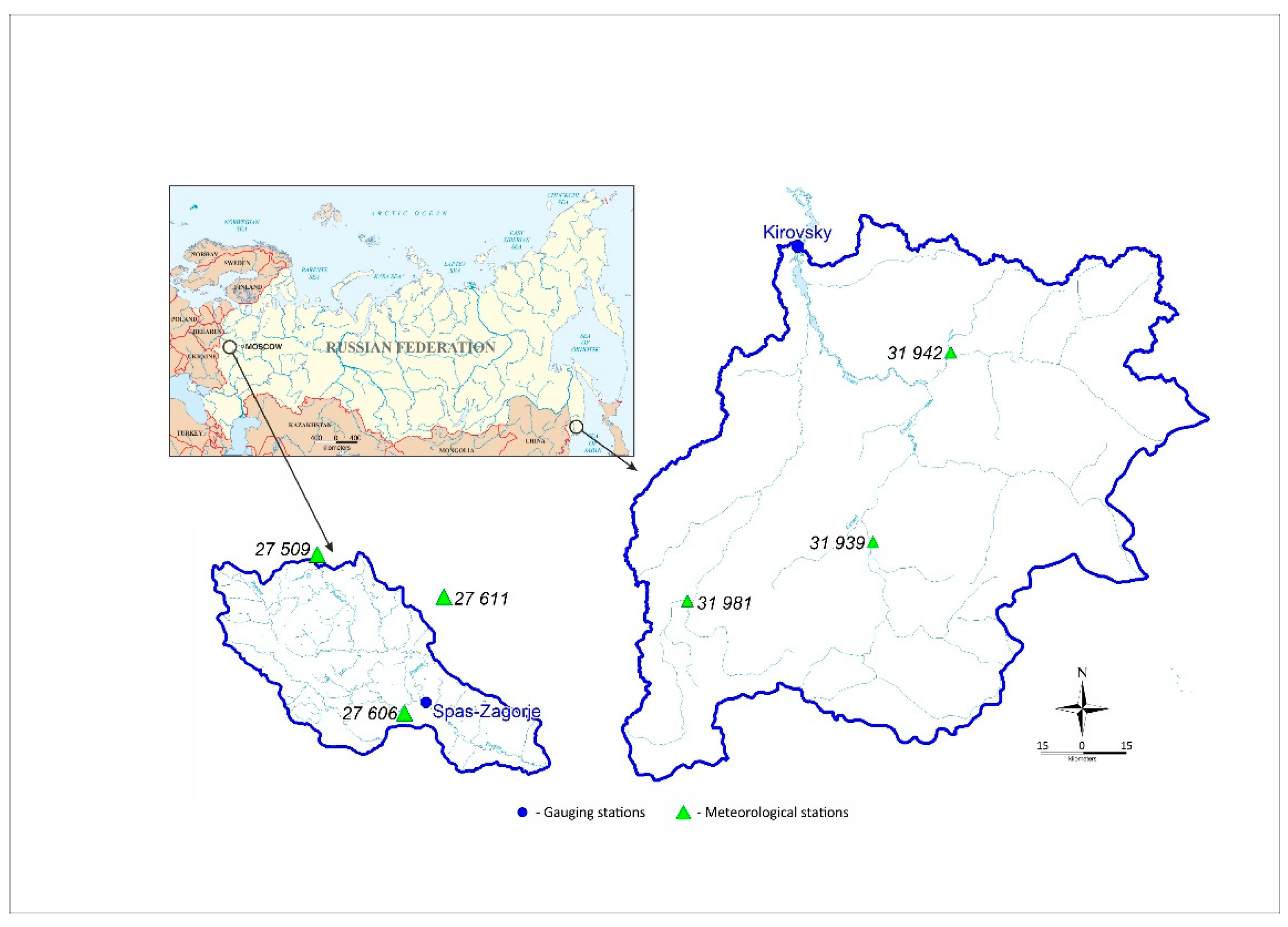
Figure 1. Location of the case study catchments.
Water 13 01696 g001
Figure 2. Combined streamflow discharge, mean catchment temperature, and precipitation plots for the Ussuri catchment in 1984 (a) and the Protva catchment in 2012 (b).
Water 13 01696 g002
Figure 3. Plots of unshuffled and shuffled datasets for the Ussuri (a) and Protva (b) rivers.
Water 13 01696 g003
Figure 4. Experiments’ flowchart (see explanations in the text).
Water 13 01696 g004
Figure 5. Model performance evaluation metrics for the Ussuri river.
Water 13 01696 g005
Figure 6. Model performance evaluation metrics for the Protva river.
Water 13 01696 g006
Table 1. The input dataset structure.
VariableColumnUssuriProtva
Predictands
Future streamflow discharge2–8 Q t + τ , τ = 1, …, 7
”Dynamic” predictors
Current and past streamflow discharge9–16 Q t τ , τ = 1, …, 7
Maximum discharge spread17–23 Δ Q m a x τ , τ = 2, …, 7
Daily precipitation amount at each weather station24–47, τ = 1, …, 7,
j = 31,939, 31,942, 31,981
P t τ j , τ = 1, …, 7,
j = 27,509, 27,606, 27,611
Basin-averaged daily precipitation amount48–55 P ¯ t τ , τ = 1, …, 7
Accumulated precipitation for the preceding period56–61τPτ, τ = 2, …, 7
”Inertial” predictors
Preceding moisture content index62 I W
Accumulated daily temperatures from the beginning of the warm period above thresholds 0, +2 и +5 °C63–65T0, T+2, T+5
Accumulated potential evaporation from the beginning of the warm period66 P E T
Table 2. Automatically (M1) and rationally (M2) selected feature sets for the Ussuri and Protva rivers.
RiverМ1М2
Ussuri Q t .   Q t 1 ,   P t 6 31981 , Δ Q m a x 7 ,   Q t 2 ,   P t 2 31942 ,
P 5 ,   Q t 5 ,   P t 31942 , Δ Qmax 4 , I W ,   P E T
Q t ,   Q t 1 ,   Δ Q m a x 7 ,   P ¯ t 1 , P 5 , I W ,   P E T
Protva Q t ,   Q t 1 ,   Q t 2 ,   Δ Q m a x 2 , Δ Q m a x 7 ,   Δ Q m a x 5 , Δ Q m a x 3 ,
Q t 3 . ,   P t 1 27509   ,   Q t 7 ,   Δ Q m a x 4 ,   P ¯ t 1 ,   I W ,   P E T
Q t ,   Q t 1 ,   Δ Q m a x 3 ,   P ¯ t 3 , T > 2 , I W ,   P E T
Table 3. Sets of all possible experiments. The conducted experiments are colored.
RiverFeature SetLMM5PMLPLSTM
UssuriM0+ ++
M1 +
M2 ++
ProtvaM0+ ++
M1 +
M2 ++
Publisher’s Note: MDPI stays neutral with regard to jurisdictional claims in published maps and institutional affiliations.