Article

Land-Cover and Climatic Controls on Water Temperature, Flow Permanence, and Fragmentation of Great Basin Stream Networks

1
U.S. Geological Survey, Washington Water Science Center, Tacoma, WA 98402, USA
2
U.S. Geological Survey, Forest and Rangeland Ecosystem Science Center, Corvallis, OR 97331, USA
3
U.S. Geological Survey, Forest and Rangeland Ecosystem Science Center, Cascadia Field Station, Seattle, WA 98195, USA
4
U.S. Bureau of Land Management, Vale District, Vale, OR 97918, USA
*
Author to whom correspondence should be addressed.
Present address: U.S. Forest Service, Northwest Forest Plan Aquatic-Riparian Effectiveness Monitoring Program, Corvallis, OR 97331, USA.
Water 2020, 12(7), 1962; https://doi.org/10.3390/w12071962
Submission received: 20 May 2020 / Revised: 2 July 2020 / Accepted: 8 July 2020 / Published: 10 July 2020

Abstract

:
The seasonal and inter-annual variability of flow presence and water temperature within headwater streams of the Great Basin of the western United States limit the occurrence and distribution of coldwater fish and other aquatic species. To evaluate changes in flow presence and water temperature during seasonal dry periods, we developed spatial stream network (SSN) models from remotely sensed land-cover and climatic data that account for autocovariance within stream networks to predict the May to August flow presence and water temperature between 2015 and 2017 in two arid watersheds within the Great Basin: Willow and Whitehorse Creeks in southeastern Oregon and Willow and Rock Creeks in northern Nevada. The inclusion of spatial autocovariance structures improved the predictive performance of the May water temperature model when the stream networks were most connected, but only marginally improved the August water temperature model when the stream networks were most fragmented. As stream network fragmentation increased from the spring to the summer, the SSN models revealed a shift in the scale of processes affecting flow presence and water temperature from watershed-scale processes like snowmelt during high-runoff seasons to local processes like groundwater discharge during sustained seasonal dry periods.

1. Introduction

Formerly intact and connected stream networks are becoming increasingly fragmented, which threatens aquatic ecosystems [1,2,3]. Most studies of fragmentation in stream networks have focused on relatively fixed barriers to movement such as culverts [4] and dams [5]. Other dynamic factors can also fragment populations of stream biota, including interactions with other species [6,7], temperature [8,9,10], and loss of surface flows [11,12,13]. Dynamic spatial patterns of fragmentation in stream networks can have variable consequences for stream biota such as increased mortality and decreased fecundity that are especially evident during droughts when stream network fragmentation is greatest [14,15,16]. As the prospect of drought becomes more likely in stream networks due to climatic changes and increasing water demands [17,18,19], it is important not only to understand the ecological consequences of drought, but to also understand how fragmentation itself arises.
The fragmentation of stream networks is best viewed as a scale-dependent phenomenon [20] across spatial scales ranging from individual reaches and temporal scales to seasons and multiple decades [21]. These patterns collectively define streamflow permanence: the extent to which the presence of surface flow is maintained at a site or across stream networks [22,23,24]. Spatial patterns of fragmentation can emerge at different levels of resolution. Coarse-grained models developed for applications over broad extents can mask finer-grained patterns of variability that exist within more limited extents [25,26,27]. Furthermore, annual and seasonal changes in hydrologic and climatic conditions can lead to dramatically different patterns of environmental suitability and fragmentation within stream networks, which have potential consequences for species vulnerability in the face of environmental extremes, such as droughts [17,21,23]. Stream network fragmentation not only prevents the movement of fish and other aquatic species, but is often also accompanied by concomitant increases in water temperature within the part of the stream network that remains wet (e.g., [28]).
Complex patterns of fragmentation in stream networks are linked to drivers that operate at different spatial and temporal scales. For example, temperature and precipitation can be strongly linked to global climatic teleconnections [29,30,31], as well as local topography, vegetation, and other factors that exert influences at very fine (<102 m) scales [19,32,33]. In terms of land and watershed management, local factors such as vegetation can be managed through direct manipulation or indirectly through managing land uses such as forestry or grazing [19,34,35]. Although ground-based measures of local drivers of fragmentation can effectively capture many of these local influences, models based on such measures cannot be easily projected and mapped to larger extents because such measures are not consistently available. Consequently, it is important to evaluate the feasibility of indicators of local processes that are derived from remotely sensed data [36].
Collectively, the challenge of defining the fragmentation of stream networks requires an understanding of (1) the drivers of fragmentation, (2) how these drivers produce patterns of fragmentation at different spatial and temporal scales, and (3) the vulnerability of human and ecological systems to fragmentation (e.g., [37]). In this study, we consider the spatial and temporal dimensions of fragmentation of stream networks in the northern and central Great Basin of the western United States, which support a subspecies of cutthroat trout (Lahontan cutthroat trout, Oncorhynchus clarkii henshawi) that is threatened by stream habitat fragmentation [38,39]. Models of species distributions based on elevation gradients [40,41] and regionally modeled hydrologic characteristics (stream discharge and temperatures [42,43]) have all pointed to contemporary and potential future fragmentation linked to warming climates as threats.
The specific objectives of this study were to (1) model seasonal variability in the influences of static and dynamic landscape characteristics from remotely sensed land-cover and climatic data on water temperature and flow permanence across stream networks and multiple (wet and dry) years in the Great Basin; (2) quantify spatial and temporal variability in fragmentation of stream networks as indicated by stream drying and temperatures; and (3) interpret the findings in light of the importance of climatic and landcover characteristics that predict stream temperatures or drying across networks. To meet these objectives, statistical models were developed to predict water temperature and predict flow presence in May, June, July, and August, when a progression of stream drying and higher water temperatures leads to the increased fragmentation of stream networks. The results of this work provide a novel illustration of how the fragmentation of stream networks in arid environments is manifested in the context of highly variable climatic contexts, such as drought [21]. Contrasts between the variable influences of drivers that can be managed (e.g., land cover) versus those that are not managed (e.g., climate, landform) provide valuable insights for future land and water management, as well as climate adaptation [44].

2. Materials and Methods
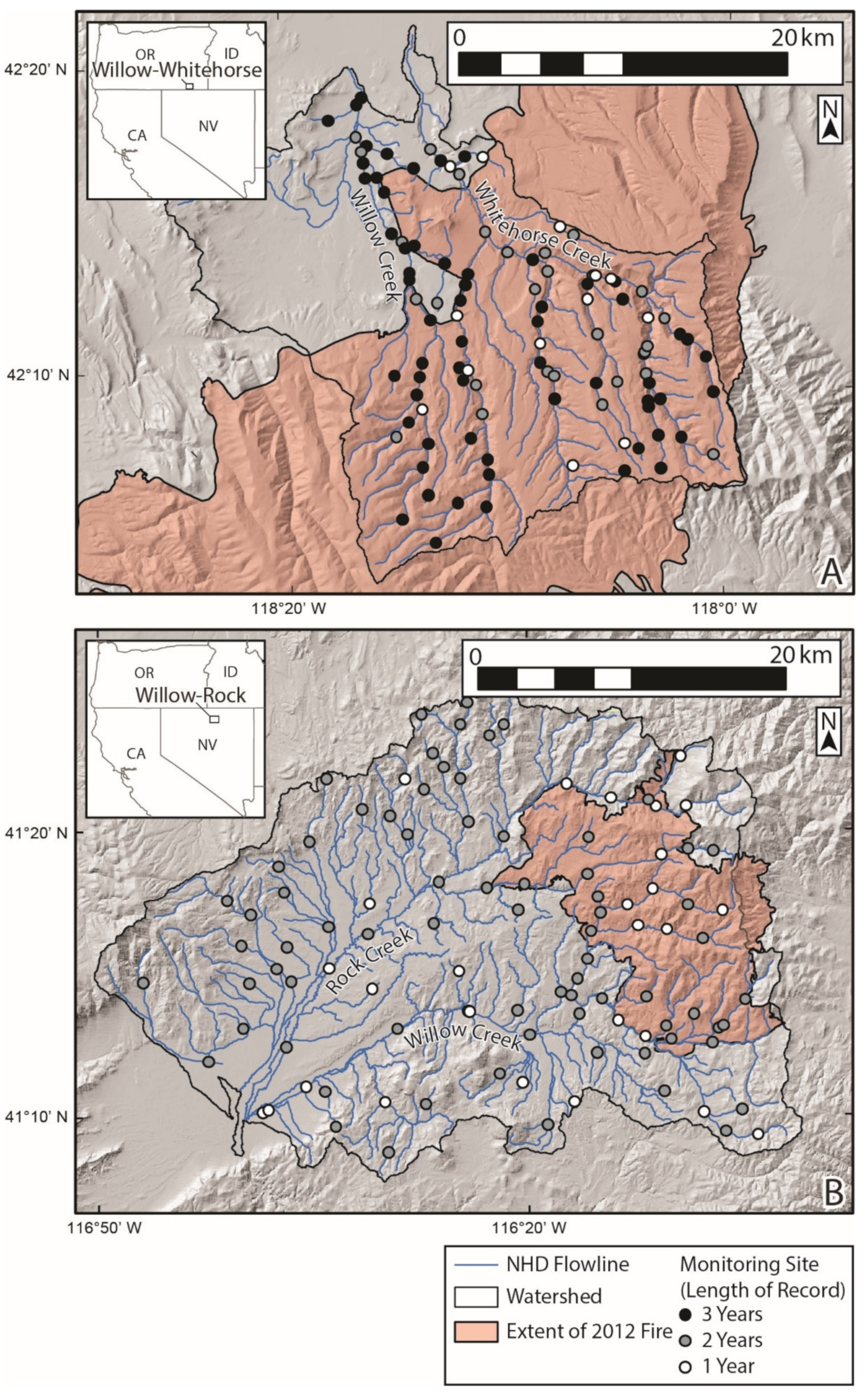
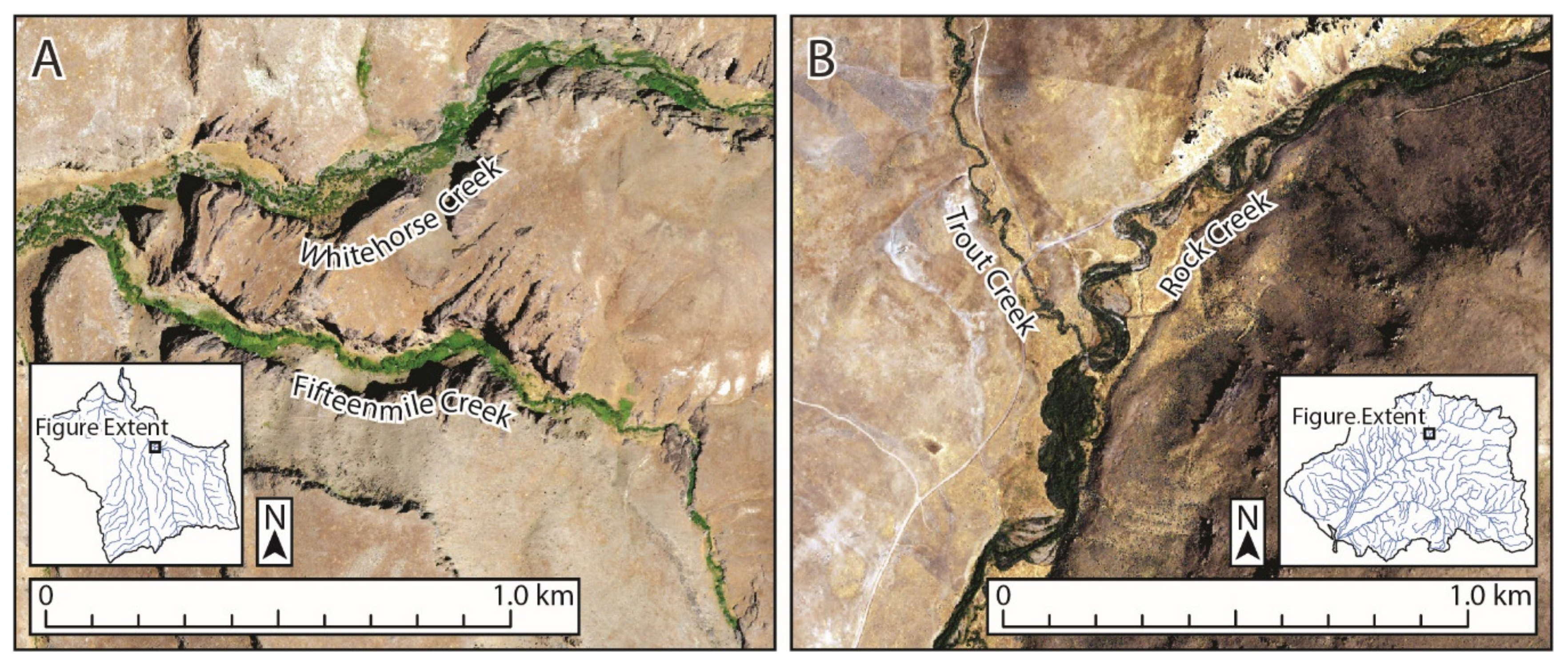
2.1. Study Sites

We studied two stream networks located within the northern and central Great Basin, USA [45,46] (Figure 1). These stream networks were selected for study because both are classified as critical habitats for Lahontan cutthroat trout, a threatened subspecies of inland cutthroat trout [47,48,49]. The Willow–Whitehorse (WW) stream network drains into pluvial Lake Coyote [50] in southeastern Oregon, and the Willow–Rock (WR) stream network drains into the Humboldt River in the Lahontan Basin of north-central Nevada. In this cold desert region, winters bring freezing temperatures, and precipitation often falls as snow [44]. Mean annual precipitation estimated by PRISM (Parameter-elevation Regressions on Independent Slopes Model) was greater in the WW watershed (390 mm) compared to the WR watershed (339 mm) for the period from 1981 to 2010 [51]. Between 2004 and 2017, mean snow water equivalent (SWE) on May 1 estimated by SNODAS (Snow Data Assimilation System) [52] ranged from 0 mm in the lower elevations of both the WW and WR watersheds to 45 and 320 mm in higher elevations of the WW and WR watersheds, respectively. During the warm and dry year of 2015, no snowpack on May 1 was present in WR and the maximum May 1 SWE in the WW watershed was 28 mm. Warm, dry summers can lead to warm (>20 °C) stream temperatures and the loss of surface stream flows [28,53,54]. The dominant land use of the contributing watersheds to these stream networks includes mining, livestock grazing (cattle and sheep), and irrigation to provide additional forage for livestock [55,56,57]. Limited surface water withdrawal occurs within both watersheds. Both stream networks were affected by wildfires in the summer of 2012, including the Holloway Fire and Willow Fires in WW and WR, respectively (Figure 1). Wildfires can cause dramatic changes in land cover, particularly riparian vegetation, which can lead to changes in stream temperatures, and potentially stream flows [28]. More detailed descriptions of each stream network can be found in [56] (WR) and [28] (WW).

2.2. Data Collection

Field data collection focused on quantifying the stream temperatures and the presence of wetted channels (as inferred by stream temperatures) [58,59]. Sampled sites in both stream networks followed Schultz et al. [28] and were distributed across accessible locations (e.g., public lands or private lands with authorized access) to include a range of environmental gradients (e.g., perennial to non-perennial streams, elevation gradients). Sampling was conducted in 2015, 2016, and 2017 at 106 sites in the WW watershed (Figure 1A) and in 2016 and 2017 (water years; 1 October to 30 September) at 109 sites in the WR watershed (Figure 1B). All sites were georeferenced using global positioning system units. Due to deployment times exceeding a year and losses of instruments placed within stream channels, we could not completely control the resulting spatial distribution of recovered loggers. Methods of statistical analysis used to predict stream temperatures and flow presence can accommodate a variety of sampling configurations [60].
Continuous records of temperature were measured at each location using data-logging thermistors (HOBO U-22 water temperature logger; Onset Computer Corporation, Bourne, MA, USA). These instruments were programmed and calibrated using protocols described by Heck et al. [61]. Temperatures were recorded at hourly intervals throughout the water year. In the field, thermistors were shielded with polyvinyl chloride (PVC) housings and secured in the deepest parts of stream channels [61] to ensure that if the thermistor was exposed to air that we could determine whether the stream dried [59]. In some locations, air temperature loggers were also deployed. These instruments were attached to nearby trees and enclosed within a radiation shield (Onset model RS1, Onset Computer Corporation, Bourne, MA, USA).

2.3. Statistical Models of Flow Presence and Stream Temperature

Spatial stream network (SSN) models, a class of generalized linear models that account for spatial autocovariance within stream networks, have been used to predict a variety of hydrologic, geochemical, and biological attributes of stream networks. Many SSN modeling efforts have focused on water temperature (e.g., [62,63,64]), in part because it is a master variable that determines the occurrence, distribution, and abundance of ectothermic species, but also because of its sensitivity to climate. SSN models applying a Gaussian distribution have been used to predict other continuous data like water chemistry [65,66] and species distribution [67]. SSN models can also be applied to non-normal data such as counts and occurrences through Poisson and binomial distributions, respectively. For example, Isaak et al. [68] developed an SSN model to predict a binary variable of bull trout (Salvelinus confluentus) presence. We are not aware, however, of any efforts to predict a binary variable of flow presence using an SSN logistic regression model. Indeed, the focus of most SSN modeling efforts has been on perennial streams, whereas flow permanence and consequences for stream network fragmentation have not been explicitly considered.
Statistical stream network (SSN) models developed by Ver Hoef and Peterson [69] were adapted for the WW and WR study areas to predict temperature and flow presence as a function of covariates that describe spatial and temporal properties of the stream network and climate. SSN models expand a standard linear model (Equation (1))
y = Xβ + ε,
where y is a vector of response variables, X is a design matrix of covariate values, β is a vector of regression coefficients, and ε is a vector of random errors to include spatially autocorrelated random effects. Inclusion of spatial structures was necessary to address spatial autocorrelation in the data that would invalidate assumptions of independence and introduce bias into parameter estimates. Ver Hoef and Peterson [69] used a moving average approach to create autocovariance models based on hydrologic distances within the stream network and propose combining them with autocovariance models based on Euclidean distance. Autocovariance models based on hydrologic distance included tail-up and tail-down models, named for the shape of the moving average function with respect to the stream network, that allow for autocorrelation based on flow-connected and flow-unconnected relationships, respectively. A number of moving average functions are available within the SSN, but in the absence of adequate data to differentiate between different spatial autocorrelation models, we limited our models to exponential moving average functions, which describe the relative influence of the moving average function over hydrologic distance. A pair of sites was considered “flow connected” if water originating from the upstream site passed by the downstream sites; if this condition did not occur, the sites were considered “flow unconnected”. Vectors of zero-mean random effects based on the Euclidean (zEUC), tail-up (zTU), and tail-down (zTD) models were added to the standard linear model (Equation (1)) such that:
y = Xβ + zEUC + zTU + zTD + ε,
The stream autocovariance models were weighted based on upstream contributing area. Two types of SSN models were developed to model different classes of response variables: continuous measures of mean monthly water temperature between May and August were modeled with a Gaussian distribution; binary indicators of flow presence between May and August were modeled with a binomial distribution through a logistic regression model.
Spatial autocorrelation within the data was evaluated using Torgegrams that quantify spatial dependence between observations that were hydrologically connected (i.e., “flow-connected”) versus observations that were hydrologically disconnected (“flow-unconnected”). Pairs of hydrologically connected observations reside on the same flow path such that water flows from the upstream site to the downstream site, whereas no common flow path links hydrologically disconnected pairs. In non-fluvial settings where a dendritic network structure and directional flow are absent, semivariograms are typically developed using Euclidean distance, but distance plotted on a Torgegram is the hydrologic distance equal to the length of the stream separating two observations.
Spatial SSN models were fit to each continuous and binary response variable using a backward stepwise regression technique [63]. Each model of mean monthly water temperature from May to August initially included all five candidate covariates, and the worst fitting non-significant (p-value > 0.10) covariates were sequentially removed until all parameters had a p-value < 0.10. A mixture of exponential tail-up, tail-down, and Euclidean autocorrelation models were included with each spatial SSN model. To evaluate the contribution of spatial autocorrelation functions, nonspatial multiple linear regression models, which excluded spatial autocorrelation functions, were developed using the same backward stepwise regression technique. Spatial and nonspatial models of flow presence were similarly developed using the backward stepwise regression technique. Random effects for year and site were included within each of the models to account for errors associated with repeated measurements at individual sites and across multiple years. Scripts and input data to run SSN models presented within this study were archived and are available for download [70]. The performance of stream temperature models, which used a Gaussian distribution, were assessed with three metrics: mean absolute prediction error (MAPE) between observed temperatures and leave-one-out cross-validation (LOOCV) predictions; root mean square prediction error (RMSPE) from LOOCV predictions; and predictive r2 calculated as the square of the correlation coefficient between observed temperatures and LOOCV predictions. The performance of logistic regression models of flow presence, which used a binomial distribution, could not be estimated with these metrics; instead, the discrimination ability of each model was estimated by calculating the area under the curve (AUC) of the receiver operating characteristic (ROC; [71]). Comparisons between spatial and nonspatial models for the same response variables were made by calculating the spatial Akaike information criterion (AIC; [72]), which penalizes models for both the number of covariates and autocovariance parameters.

2.4. Flow Presence and Temperature Metric Development

2.4.1. Diagnosis of Flow Presence/Absence

Differences in the range of daily temperature variability that occur due to the contrast between the heat capacity of air and water have previously been exploited to classify wet and dry conditions within streams [59,73,74]. We used complementary graphical and analytical techniques to determine if observed temperatures recorded by in-channel thermistors indicated wet or dry conditions in the stream channel at a daily interval. Prior to analysis, temperature measurements recorded before and after thermistors were deployed in the stream channel were removed from each record. For each site, hourly temperature measurements, daily temperature range, and daily standard deviation temperature measurements were summarized from May to August of each year and visually inspected to identify abrupt transitions in the daily range and standard deviation that could potentially indicate a change in state (e.g., wet to dry, dry to wet). In addition, temperatures below 0 °C or above 30 °C were classified as dry in most instances.
The graphical determination of wet and dry conditions at each temperature measurement site was complemented by an analytical approach based on comparison of the daily standard deviation of hourly temperature measurements recorded by in-channel thermistors to that recorded by paired out-of-channel thermistors that recorded nearby air temperature. Most in-channel thermistors were compared to a nearby air temperature thermistor, but in the absence of a nearby air temperature thermistor, air temperature data were obtained from nearby weather stations. To smooth the variability in the daily time series, we calculated weekly moving averages of daily standard deviations for stream channel and air temperatures.
The ratios of the daily standard deviation of stream channel temperature (σTw) to the daily standard deviation of air (local or regional data) temperature (σTa) were used to identify a specific cutoff value for ratios of σTwTa and diagnose dry conditions. To select an efficient cutoff, electrical resistance data indicating known drying (or wetting) cases from WW were used [59]. A numerical search was performed on the values of potential cutoffs of σTwTa between 0.5 and 1.0, with a step size of 0.01. We found that, in WW, a cutoff ratio of 0.8 or greater produced the highest classification rate, as measured by the proportion of correct wet/dry classifications out of the total number of day-site combinations classified (Figure 2). The classification rate of the analytical technique using a 0.8 cutoff ratio was about 90 percent based on electrical resistivity data in the WW watershed between April and August, which was slightly greater than the classification rate of the graphical technique over the same time period. Therefore, where a discrepancy existed between the wet/dry classification assigned by the analytical and graphical techniques, the analytical technique superseded the graphical technique. By adopting a range of subjective visual and more objective numerical methods for diagnosing flow presence/stream drying, we were more confident in identifying locations that stayed dry or wet during the season of interest (May–August), or that changed in state. These methods identified the presence or absence of water within the channel and did not differentiate between moving and standing water.

2.4.2. Summary of Temperatures and Flow Presence/Stream Drying

Continuous response variables for water temperatures, including mean monthly water temperatures for May (MayTw), June (JunTw), July (JulTw), and August (AugTw) were calculated at sites that included data for at least 90 percent of the month and at which water was inferred to be present for all days of the temperature record. Sites that included any dry days were excluded. The total number, for all years, of temperature measurement observations included for each of the continuous response variables was 244 (MayTw), 251 (JunTw), 217 (JulTw), and 194 (AugTw), indicating a decrease in the number of stream channels with flow present from May through August. At each temperature measurement site, a binary response variable of flow presence was calculated on May 15 (May15Wet), June 15 (Jun15Wet), July 15 (Jul15Wet), and August 15 (Aug15Wet), where zero denotes a dry channel and one denotes a wet channel. The condition of flow presence was determined on a single day of each month to remove ambiguity regarding the duration of drying at individual sites.

2.5. Model Covariates and Hydrography

Heat is transferred into and out of a stream by radiative, conductive, convective, and advective processes, which differ in their relative influence depending on the climatic, hydrologic, and geomorphic regime of a stream and its contributing watershed. The temperature of water at a point in the stream network indicates the accumulated gains and losses of heat through these processes [75]. Similarly, stream discharge, as well as the presence of water itself, results from the cumulative water input to and outflow from the stream. Five covariates related to physical processes hypothesized to affect stream temperature and flow presence (snowmelt, groundwater inflow, evapotranspiration, riparian vegetation abundance, interannual variability in discharge, and interannual variability in air temperature) were introduced as covariates into predictive models of stream temperature and flow presence (Table 1). Candidate covariates represented both temporal and spatial variability in the processes affecting water temperature and flow presence. Multicollinearity within model covariates was assessed by calculating variance inflation factors (VIF) for each model. VIF for model covariates were generally low (<5) and none exceeded 10, above which the strong dependence between covariates impedes model parameterization and interpretation [76].
Landscape, hydrologic, and climatic variables were considered for inclusion as covariates in statistical models of water temperature and presence. Landscape variables such as elevation and drainage area emerged as significant covariates in previous statistical models of stream temperature (e.g., [63,64,77,78]) but are related to multiple physical processes that confound interpretation of their mechanistic link to water temperature. For example, elevation is related to several factors that may influence water temperature, including air temperature, precipitation, snowpack accumulation, and the type and distribution of riparian vegetation. Although variables like elevation and drainage area may explain much of the variance in water temperature throughout a drainage network, they cannot be influenced themselves by management actions. Consequently, elevation and drainage area were excluded from consideration as covariates within models presented here in favor of variables that can be more directly linked to specific physical processes affecting stream temperature.
Three covariates, which varied both spatially and temporally, were calculated annually for each year of observed data within each of the study watersheds: presence of snow in contributing watershed on 1 May (SWEws); mean riparian normalized difference vegetation index (NDVI; NDVIrip); and mean riparian evapotranspiration (ET; ETrip). Gridded snow water equivalent on 1 May was estimated by SNODAS [52] at a 1-km resolution for each year of observations in the model. SWEws was defined as a categorical covariate of the presence or absence of snow on 1 May in the contributing watershed upstream of each temperature and flow presence observation. During the spring, snowmelt lowers the stream temperature and the potential for a loss of surface flow by contributing cool water to the stream network. The relation between vegetation and evapotranspiration with water temperature and presence of surface flow, however, is more complex and feedback mechanisms between the presence of flow, the growth of riparian vegetation, and evapotranspiration exist. Vegetation reduces the input of solar radiation, which typically comprises the largest input of heat to smaller streams [79]. The presence of vegetation, however, may also indicate the presence of shallow groundwater levels [80] that may be associated with cool groundwater inputs and reduced stream temperatures. The evapotranspiration of water from the riparian zone reduces streamflow [81], thus decreasing the potential for surface flow presence, but also contributes to evaporative heat loss thus cooling the stream. ET was estimated using the Operational Simplified Surface Energy Balance (SSEBop) model [82] with 30-m resolution Landsat 8 scenes with less than five percent cloud cover. NDVI, an index of vegetation cover over a landscape derived from the ratio of reflectance of red and near infrared radiation measured by satellites, was estimated from the same 30-m resolution Landsat 8 scenes used by SSEBop to estimate ET. NDVI values range between −1 and 1 with negative values indicating a lack of vegetation. NDVI and ET were estimated over the four-month period from 1 May to 1 September for each year from 2015 to 2017 and assigned to temperature and flow presence observations of the corresponding year. The three-month estimation period for the NDVI and ET increased the reliability of model estimates over shorter (e.g., monthly) time periods [83]. NDVI and ET were then spatially averaged for a 200-m wide riparian corridor for the stream network upstream of each temperature and flow presence observation to generate the riparian-averaged covariates NDVIrip and ETrip. The extent of riparian vegetation in both the WW and WR watersheds varied substantially from 10 m or less in some headwater drainages to nearly 200 m in parts of the mainstem streams (Figure 3). The 200-m wide riparian corridor width to calculate NDVIrip and ETrip was selected to provide a consistent area around the WW and WR drainage networks that encompassed the potential zone of influence of vegetation on riparian shading and evapotranspiration.
To account for interannual climatic variability, discharge and air temperature were introduced as spatially invariant, temporal covariates. The mean monthly temperature (MonthTa) from May to August was averaged over each study watershed from PRISM climate data [51] to account for the expected positive relationship between air and water temperature. We expected discharge to have a negative relationship with stream temperature and was accounted for by introducing monthly averaged unit discharge (discharge per unit contributing area; MonthQ) as a covariate. Because no stream gages existed within either of the study basins during the period of water temperature and presence observations, unit discharges were calculated for neighboring watersheds with contemporaneous discharge data. The mean monthly unit discharges calculated for USGS (U.S. Geological Survey) gage 10352500 (McDermitt Creek near McDermitt, NV, USA) and USGS gage 10321940 (Maggie Creek above canyon near Carlin, NV, USA) [84] were assigned to temperature and flow presence observations for the WW and WR watersheds, respectively.
The hydrography of the WW and WR watersheds was imported from the National Stream Internet (NSI; [85]) data set, which was processed from medium-resolution NHDPlusV2 [86] to meet SSN model requirements for topological consistency by removing braided and diverging channels and confluences with more than two tributaries. Spatial Tools for the Analysis of River Systems (STARS; [87]) was used to further pre-process the spatial and topological attributes for SSN model hydrography, and the stream temperature and flow presence measurement and prediction sites. STARS was then used to create an SSN object for the SSN package version 1.1.13. [88] in R [89].

3. Results

3.1. Flow Presence and Temperature

The annual recovery rates of deployed water temperature loggers ranged from 70 to 97 percent in WR (2017) and WW (2015), respectively. The observed mean monthly water temperatures across all site-years were lowest in May (10.3 °C) and highest in July (15.7 °C); whereas the percentage of sites where flow was present was highest on 15 June (64 percent) and lowest on 15 August (52 percent). The highest observed mean monthly water temperatures occurred in 2015 for all months between May and August, but the lowest observed mean monthly temperatures occurred in 2017 during May and June and in 2016 during July and August. The observed mean monthly temperatures from all months were lowest in the WR watershed and highest in the WW watershed, which was lower in elevation but was more northerly in aspect and at a higher latitude.
Flow presence also varied across watersheds and years (Table 2). Overall, the WW watershed exhibited a greater proportion of sites where surface flow was present on 15 August (0.63, 0.67, and 0.64 in 2015, 2016, and 2017, respectively), whereas WR exhibited a much lower (and variable) proportion of sites where flow was present on 15 August (0.23 and 0.38 in 2016 and 2017, respectively). Most locations remained in the same state across years and seasons, although we observed a few sites that changed state across years (Table 2).

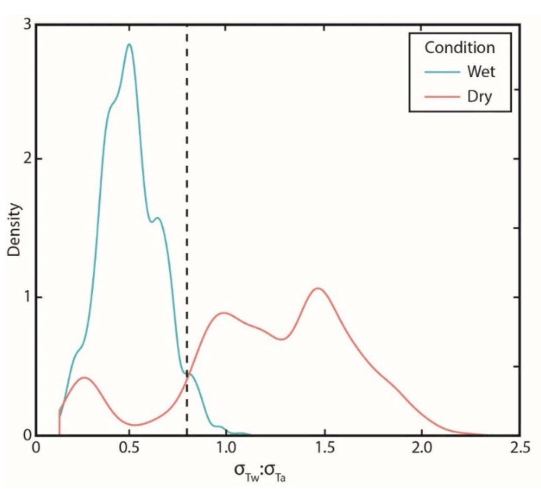
3.2. Seasonal Changes in Spatial Dependence of Stream Temperature

Torgegrams of mean monthly stream temperature for the four time periods (MayTw, JunTw, JulTw, and AugTw) were evaluated for individual years from 2015 through 2017 (Figure 4). For flow-connected sites, semivariance of MayTw, JunTw, JulTw, and AugTw was low at short hydrologic separation distances and increased with distance, indicating a broad-scale trend in water temperature. Conversely, spatial autocorrelation was evident among flow-unconnected sites in May and June and leveled off at relatively short (~15 km) separation distances, indicating smaller-scale patchiness in water temperature. Spatial dependence among flow-unconnected sites was more pronounced in May and June (Figure 4A,B) and became progressively less apparent in July and August (Figure 4C,D). These relations were largely consistent across years.

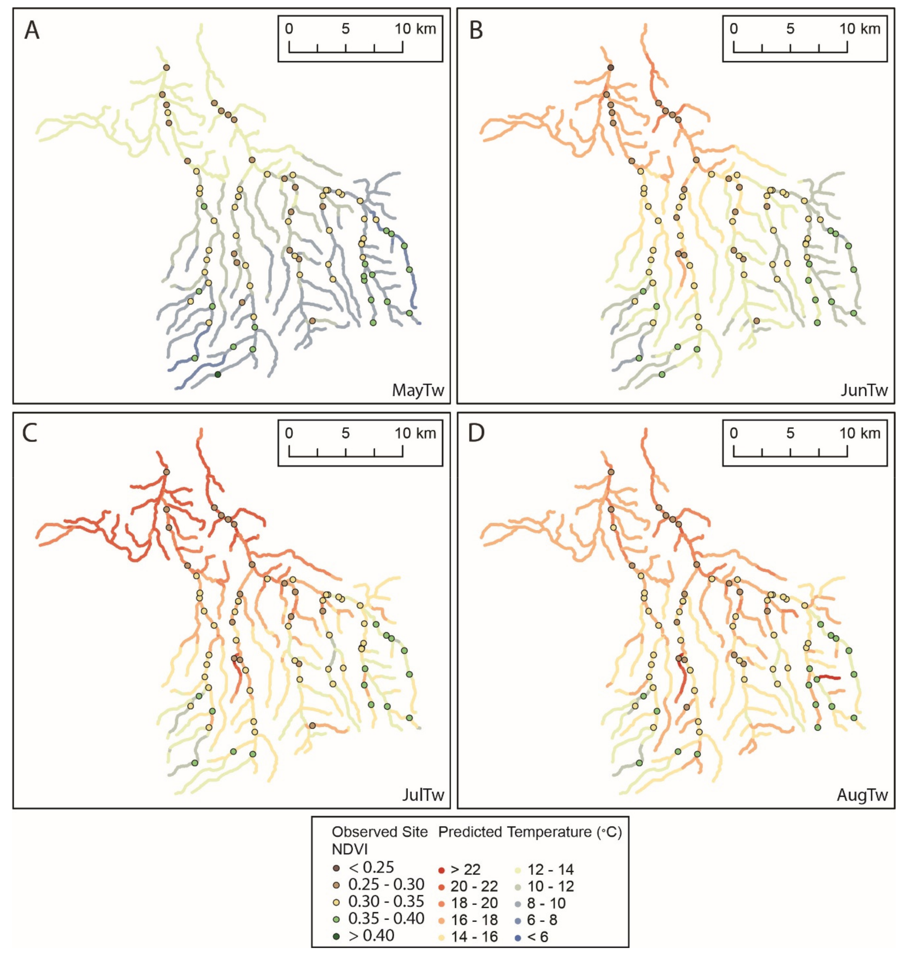
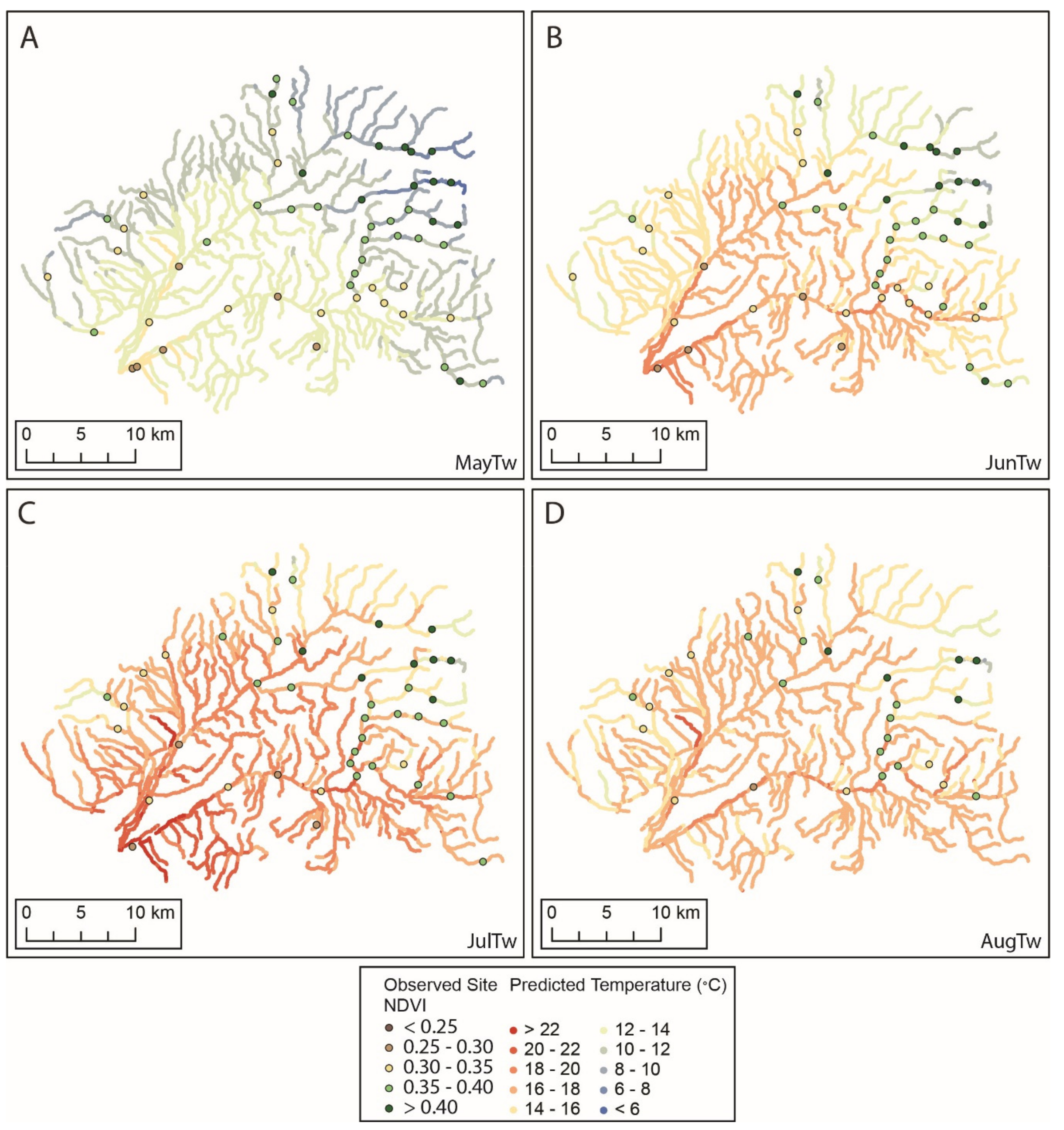
3.3. Models of Stream Temperature

Spatial stream network models outperformed nonspatial multiple linear regression models of mean monthly water temperature for all four months modeled as measured by higher LOOCV r2pred, lower RMSPE, and lower MAPE (Table 3). The AIC scores of spatial models were 14 to 217 points lower than nonspatial models even after accounting for the additional autocorrelation function parameters included in the spatial models. Predictive performance of both spatial and nonspatial models was highest for the MayTw models (spatial model LOOCV r2pred: 0.89) and lowest for the AugTw models (spatial model LOOCV r2pred: 0.66); similarly, the relative improvement of AIC scores from nonspatial to spatial models (i.e., by including spatial autocovariance structures) was highest for the MayTw models (ΔAIC: 217) and lowest for the AugTw models (ΔAIC: 14). The relative proportion of variance explained by different spatial structures changed correspondingly between models of MayTw and AugTw. Although the Euclidean autocovariance structure explained 67 percent of variance within the MayTw model, it did not explain any variance within the AugTw model. The tail-up and tail-down autocovariance structures based on the stream network explained the increasing proportions of variance from the models of MayTw to AugTw.
The percentage of variance explained by covariates was highest for the spatial model of JunTw (57 percent) and lowest for the spatial model of AugTw (16 percent). The relation between covariates and mean monthly water temperatures in fitted models was both consistent and inconsistent with a priori hypotheses. For models of all mean monthly water temperatures, NDVIrip was consistently among the most significant covariates and was associated with cooling water temperature for each month (Table 1). SWEws was significant in the spatial models of MayTw and JunTw, but not for any of the other months, indicating the timing of peak snowmelt in both study watersheds. The mean monthly temperature was significant in all spatial models of mean monthly water temperature except for the model of MayTw, but its effect was opposite in sign of our hypothesis for the models of JulTw and AugTw. Similarly, mean monthly discharge was significant in spatial models of MayTw, JulTw, and AugTw, but its effect was opposite in sign compared to our hypothesis for the spatial models of JulTw and AugTw.
The mean monthly water temperatures from May through August were predicted at unsampled locations at 100-m intervals to develop a continuous map of temperature across the entire stream network of the WW (Figure 5) and the WR watersheds (Figure 6). The mean monthly water temperatures from May through August were generally higher in the WR watershed than in the WW watershed. In general, headwater tributaries where NDVI was higher were cooler than mainstem streams where NDVI was lower for all modeled months in both watersheds. The relative difference in temperature between headwater and mainstem streams increased from May through August, and longitudinal heterogeneity in predicted water temperatures also increased from May through August. The mean monthly water temperature was calculated for all stream segments contained within the NSI hydrography, but the presence of water within these segments varied from May to August, as estimated by models of flow presence.

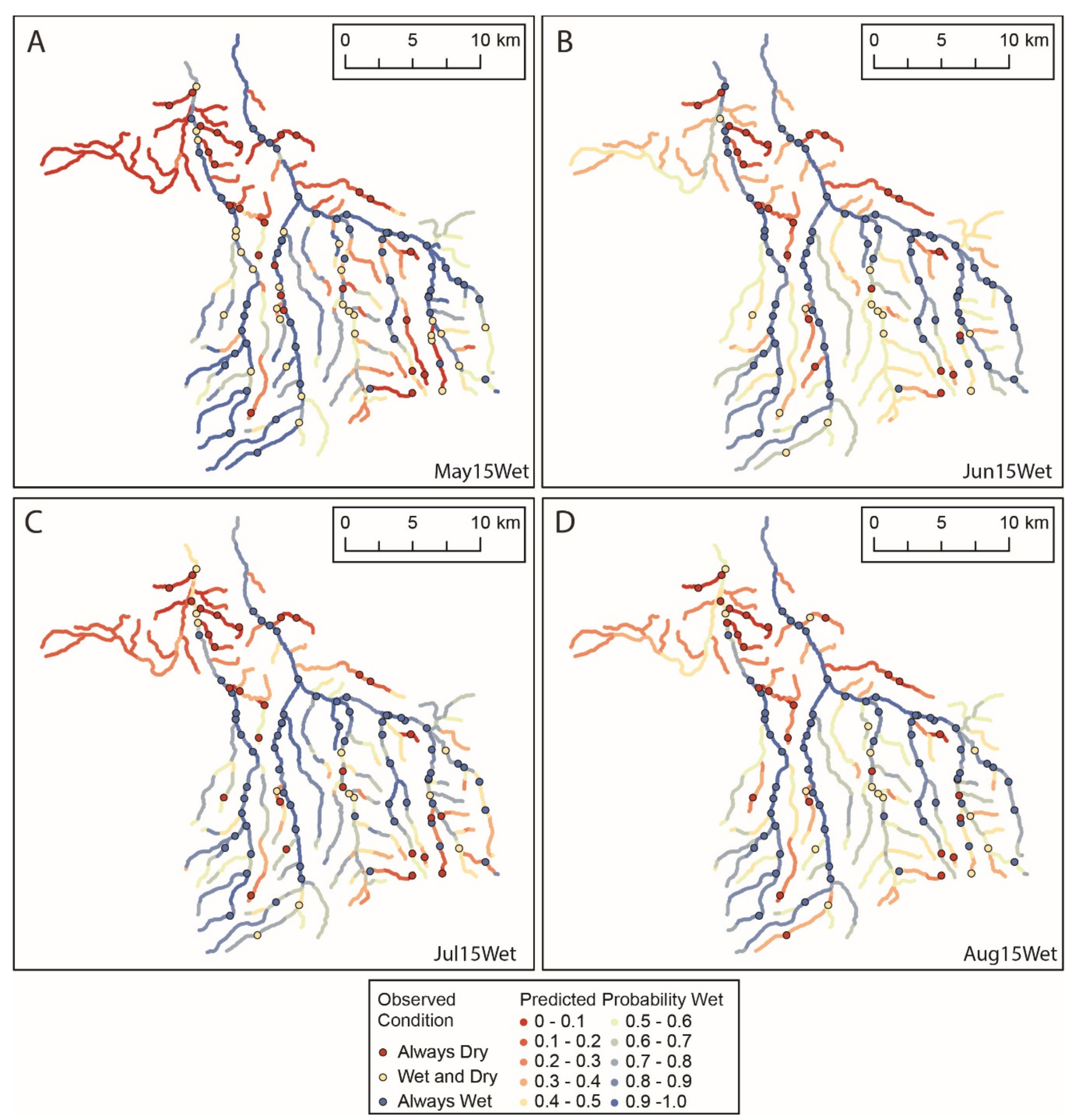
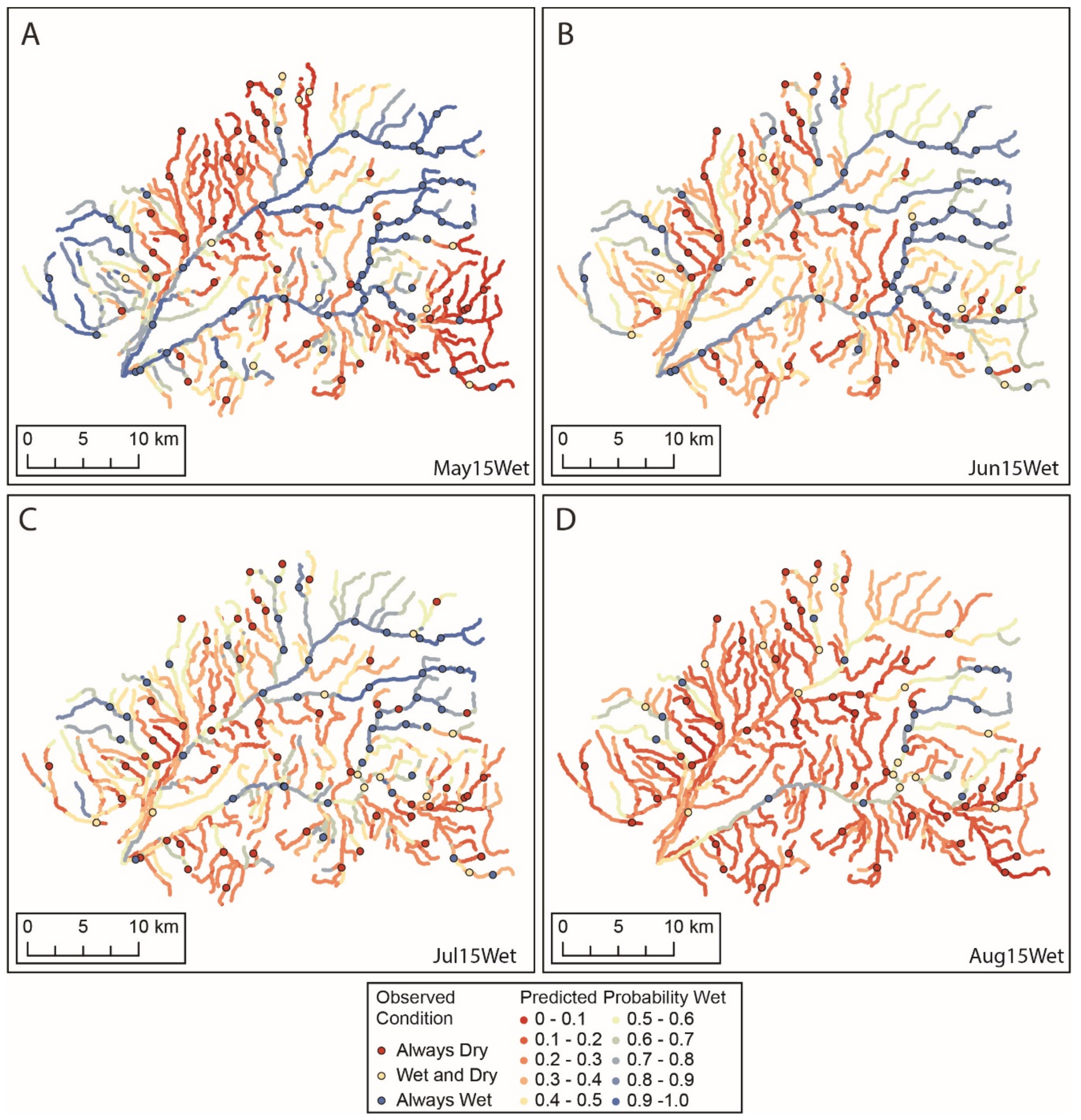
3.4. Models of Flow Presence

The SSN logistic regression models fitted to flow presence data are summarized in Table 4. These models predict the probability of flow on the days that we selected for this analysis: 15 May, 15 June, 15 July, and 15 August. The predictive performance of nonspatial models of flow presence was high within the area under curve (AUC) of the receiver operating function (ROC) between 85 percent (May15Wet model) and 91 percent (Jun15Wet model) indicating that flow presence models discriminate well between wet and dry conditions. The inclusion of spatial autocovariance structures increased the predictive accuracy of models of flow presence (Table 4), but only marginally. For example, the AUC of the ROC calculated for the Aug15Wet model increased by seven percent, which was the maximum for all four models of flow presence. NDVIrip was consistently the most significant covariate for all models of flow presence and was positively related to flow presence, as hypothesized. SWEws was also significant in the May15Wet model and was positively related to flow presence. The mean monthly discharge was significant in the Aug15Wet model, but not in any of the other models.
The probability of flow presence was predicted at 100-m intervals across the stream networks of both watersheds on 15 May, 15 June, 15 July, and 15 August (Figure 7 and Figure 8). The most spatially extensive and contiguous wetted stream network was predicted by the 15 May model (Figure 7A and Figure 8A), whereas the least spatially extensive and most fragmented stream network was predicted by the 15 August model (Figure 7D and Figure 8D). The flow presence and fragmentation were not consistent between the WW and WR watersheds but were more pronounced in the WR watershed (Figure 8). The probability of flow presence predicted by the August 15 model exceeded 50 percent throughout most of the mainstem streams of the WW watershed including Willow, Whitehorse, and Little Whitehorse Creeks and their major tributaries, with limited stream drying and fragmentation predicted. In the WR watershed, flow was predicted to be present throughout mainstem streams, including Willow and Rock Creeks, as well as smaller tributaries like Frazer Creek by the 15 May model, whereas a predicted flow presence exceeding 50 percent was limited to Willow Creek and several headwater streams by the 15 August model.

4. Discussion

In this study, we sought to quantify annual, seasonal, and spatial variability in stream temperatures and flow permanence (i.e., the maintenance of flow presence) in drought-sensitive stream networks, and to quantify how different landscape processes (climate and land cover) drive stream-network fragmentation. Our results show that stream temperature and flow permanence varied seasonally and spatially at local scales (Figure 5, Figure 6, Figure 7 and Figure 8). These findings are consistent with previous work in the region and in similar environments elsewhere, including studies in the WW basin [28,59] and other stream networks (e.g., [90,91,92]), where marked patterns of variability occurred at even the finest level of observation [26,77,93,94]. Although quantifying such patterns of variability can require enormous effort, a larger challenge lies in understanding the processes that drive them. Here, we considered two classes of landscape processes (Table 1) that we were able to quantify consistently with available spatial data across the two networks studied.
The major drivers of stream temperatures and streamflow permanence are climatic in unmodified rivers. Influences of climate are typically evident at broad regional scales [94]. Broad-scale models of stream temperatures [64,95,96] and streamflow permanence [97] have identified the importance of air temperatures and precipitation, respectively, as strongly associated with these responses. We focused on a smaller spatial extent, however, and associations between stream temperatures and streamflow permanence were not always in agreement with predictions based on hypothesized effects of climatic drivers (Table 1). For stream temperatures, the May snow water equivalent was important for temperatures in May and June, but not for later months (Table 3). This may be expected as the snowpack is largely depleted after June in these watersheds, and other processes can play a greater role in driving hydrologic responses. Unlike snow water equivalent, associations with monthly air temperatures and stream discharge were not consistent across months. Although climate is an important higher-level driver of stream temperatures and streamflow permanence at broader scales [94], variation in the influences of these factors on hydrologic processes within each of the networks studied herein may not have been great enough to detect associations.
We considered two indicators of the influence of land cover on stream temperature and streamflow permanence: a measure of evapotranspiration, and vegetation cover as indicated by NDVI. Although evaporation represents a net export of heat from streams [75], rates of evapotranspiration increase as temperature increases and therefore may be associated with warmer stream temperatures. Evapotranspiration can also be strongly linked to water that is potentially available to streams, particularly in arid regions [98,99]. In this study, however, we did not detect an association between evapotranspiration and water temperature or streamflow permanence. Overall, these findings lead us to conclude that the measure of evapotranspiration we employed does not have a direct, strong influence on stream temperatures or streamflow permanence, although evapotranspiration can be a significant driver of both responses. In contrast to evapotranspiration, riparian NDVI, a variable that could indicate multiple hydrologic processes (Table 1), was consistently associated with both temperature and streamflow permanence across all seasons.
As hypothesized, riparian NDVI was related to cooler water temperatures and an increased probability of surface streamflow. NDVI, which correlates with vegetation productivity, has been widely used to remotely assess vegetation distribution and its interactions with other parts of ecosystems [100]. In small streams such as those studied here, riparian vegetation plays a primary role in regulating temperatures by reducing shortwave radiation from solar insolation through shading [101,102,103]. Although NDVI does not explicitly resolve changes in shortwave insolation due to riparian shading, such as cumulative riparian solar exposure, it does indicate the presence or absence of riparian vegetation that regulates stream temperature in a similar manner to the percentage of riparian canopy cover. In an arid landscape, NDVI may not only differentiate between areas with and without riparian vegetation, but may also reveal areas of shallow groundwater [57,104]. Shallow groundwater, which sustains vegetation and increases NDVI, may discharge into streams where it both increases the probability of flow permanence and buffers summer stream temperatures by contributing cool groundwater discharge to streams.
More broadly, NDVI has been directly applied across the Great Basin to quantify habitats for terrestrial species, such as the greater sage-grouse (Centrocercus urophasianus; [105,106]), and as an indicator of (1) riparian recovery in response to improved grazing management, influences of beaver, and wildfire [56,57,80,107,108]; and (2) longer-term climate-related changes in hydrologic and vegetative conditions [104,109]. Interestingly, direct associations between NDVI and instream responses of macroinvertebrates or fish can be less apparent [110,111]. Based on our findings and those of many prior studies, however, NDVI has broad potential as an indicator of riparian and instream conditions in the Great Basin, though additional work is needed to refine spatial and temporal variability in such relationships [112]. For example, in WW, field-based data on pre- and post-burn responses of stream temperatures to a large and severe wildfire showed a high degree of variability [28]. In our study, unexplained variability in stream temperature (Table 3) may indicate the importance of local processes not captured by NDVI or other model covariates.
The extent to which stream networks are fragmented depends on the specific ecological responses of interest. The streams that we studied are designated critical habitats for Lahontan cutthroat trout, a threatened species [111]. The distribution of this species is strongly influenced by water temperature and perennial stream flows [39,41]. Other species may respond less to temperature and more to the presence of available surface water. We were generally successful in developing models to predict stream temperatures and streamflow permanence. Although we collected high-resolution stream-temperature data within the study networks, predictions of stream temperature were statistically less precise than those for a regional model of stream temperature [64]. In other words, the finer-grained variability of temperature within local watersheds can be very complex and more difficult to predict than variability at larger spatial extents. This result underscores the importance of considering scale in applying results from regional [64] and local (our study) models of in-stream hydrologic responses [21] to understand stream-network fragmentation. Measures of model performance for predicting stream temperatures declined from spring (May) through late summer (August), perhaps indicating that as the hydrologic stream network became more fragmented (intermittent), local processes not captured in our spatial covariates were driving localized heat budgets at scales of 10–100 m. In contrast to stream temperature, our predictions of streamflow permanence (probability of drying) were generally much more precise than a regional model of flow permanence [97], particularly in June, July, and August (Table 1 and Table 2).
As stream networks become progressively fragmented during the summer dry season, local processes may become increasingly important influences on water temperature and flow permanence as the contribution of processes operating at the extent of watersheds decreases [92,113,114]. Because precipitation is limited in the summer and the snowpack has largely melted, groundwater discharge to streams likely accounted for a larger proportion of stream discharge as the contribution of surface runoff decreased from spring through summer. As a result, covariates related to snowmelt such as SWEws were significant in May and June, but not in July and August water temperature and flow permanence models. Unlike surface runoff, which is broadly distributed across the landscape, groundwater discharge may be very localized within stream networks.
In our study of stream networks, the effect of progressive fragmentation on water temperatures was apparent across seasons (Figure 7 and Figure 8). The spatial autocorrelation among flow-connected sites, indicated by increasing semivariance at greater separation distances, was present between May and August (Figure 4). In contrast, spatial autocorrelation among flow-unconnected sites was present at distances of less than 15 km in May but became less pronounced in July and August. This suggests that watershed-scale processes and flow connectivity may be relatively more important drivers of stream temperature in May and June than in July and August. This seasonal change in the relative roles of watershed versus local processes was apparent not only in the changes in spatial autocorrelation depicted in the Torgegrams, but also in the significance of covariates and the relative predictive power of stream temperature models.
We hypothesize that, as stream networks become increasingly fragmented, coarse-scale covariates, such as those used in our study, may not adequately capture the localized processes contributing to observed temperature patterns [21,90] because drying of surface flows changes the hydrologic connections between points in the stream network. Although hyporheic connections may exist, streamwise autocovariance functions may change when surface flows are fragmented. As a result, the LOOCV r2pred of stream temperature models was greatest in May (0.89) and progressively decreased through August (0.65). Concomitant with this decrease in predictive power was a decrease in the percentage of variance explained by autocovariance structures from May to August. For streamflow permanence, the inclusion of spatial structures only marginally increased the predictive performance of models (Table 4). The probability of flow presence decreased throughout the network in both the WW and WR watershed from May to August, but a greater proportion of the streams in the WW watershed remained wet from May to August. Paradoxically, the snowpack in the WW watershed was consistently less than in the WR watershed, but because runoff from snowmelt was largely depleted by June, other processes (e.g., groundwater flux) sustained late summer streamflows.
Although much progress has been made toward understanding terrestrial responses to changing climates, much less is known about water quality and availability in streams, which are important not only to fish, but also to a host of wildlife species and other valued ecosystem functions [21,37,115]. This is specifically true of the Great Basin, an arid region where surface water is already chronically scarce [44]. As climate-related drought becomes more likely in the region [116], stream networks will be fragmented and water scarcity will increase in space and time [24,117,118].
In our study, we predicted streamflow permanence using widely applied statistical methods with relatively simple landscape covariates such as NDVI. However, it may be difficult to attribute NDVI to specific, localized processes that influence water availability or stream temperature. Nevertheless, NDVI is an important indicator of changes in land management or influences of wildfires and can be used to track the effectiveness of land and water management actions in a changing climate [56,57,80,107,108]. Additional predictors that are similar to NDVI but finer in spatial resolution are needed to explain the high degree of spatial variability in stream temperature and flow presence that we observed. For example, covariates that characterize localized heat budgets based on shade and groundwater/surface water interactions are needed for better predictive models. Moving from publicly available spatial data sources to high-resolution remotely sensed data (e.g., airborne thermal infrared remote sensing, lidar, and aerial photography) and field measurements may be costly and logistically challenging. However, such efforts may be warranted because broad-scale models of stream temperature may not be sufficient for identifying local patterns of warming and multiscale thermal refuges that are critical to many species in fragmented, increasingly drought-prone landscapes [21,28].

5. Conclusions

This study provides novel insights into the fragmentation of stream networks with respect to patterns of stream temperature and flow permanence. Although SSNs have been used to predict stream temperature in multiple studies, we are unaware of previous efforts to use an SSN logistic regression model to predict flow permanence for a comparison to contemporaneous stream temperature. The high-density water temperature and flow presence datasets used to develop the SSN models presented within this study enabled us to consider the potential drivers of stream temperature and flow permanence at finer spatial scales than has previously been investigated. This study design made it possible to (1) explain fragmentation in terms of drivers that operate at different spatial and temporal scales and (2) evaluate a seasonal shift in processes that drive water temperature and flow permanence—from snowmelt in the late spring to riparian shade and groundwater discharge in the summer. Quantifying the seasonal and interannual variability in stream temperature and streamflow permanence is critical to understanding climatic variability and vulnerability, especially in the context of drought, which is a concern for aquatic ecosystems globally [17] and locally in the Great Basin [44]. Spatial scaling is also important because coarse-grained models of climate exposure (e.g., stream temperature and flow presence) may not reveal granular details, such as localized refuges that can be critical for species survival during stressful periods [21,119,120]. In streams, it is well known that such refuges can be common [25,77,94]. Accordingly, although fragmentation is often described as a threat to species persistence in stream networks [1,2,3], thermal heterogeneity can also create a patchwork of refuges that can carry species through stressful exposures. Our findings highlight the need for catchment-wide, high-density observations of water temperature and flow permanence to quantify thermal heterogeneity and predict the effects of finer-scale covariates such as riparian canopy condition, channel morphology, and groundwater/surface water interactions. Modeling these finer-scale drivers of stream temperature and flow is important to address scales where land managers can effect change [26] and scales that are important to species vulnerability to hydrologic change [21].

Author Contributions

Conceptualization, A.S.G., J.B.D., C.E.T., T.A.; methodology A.S.G., J.B.D, C.E.T., D.P.H.-W., J.T., J.M.; formal analysis, A.S.G., J.T., J.M.; investigation, A.S.G., J.B.D., C.E.T., D.P.H.-W., M.P.H., J.T., J.M.; data curation, A.S.G., D.P.H.-W., J.T., J.M.; writing—original draft preparation, A.S.G., J.B.D.; writing—review & editing, A.S.G., J.B.D., C.E.T., D.P.H.-W., M.P.H., J.T., J.M., T.A.; visualization, A.S.G.; supervision, J.B.D.; project administration, J.B.D. All authors have read and agreed to the published version of the manuscript.

Funding

This work was funded by the Bureau of Land Management (Oregon and Washington State Office and Vale District Office), the U.S. Fish and Wildlife Service (Northern Nevada Field Office), and the Great Basin Landscape Conservation Cooperative.

Acknowledgments

Field support was provided by the Northwest Forest Plan Aquatic and Riparian Effectiveness Monitoring Program and the Oregon Department of Fish and Wildlife. U.S. Geological Survey field crews included B. Sempert, A. Berthold, L. Schultz, and J. Pearson. M. Friedrichs with the U.S. Geological Survey’s Earth Resources Observation and Science Program provided assistance with the development of evapotranspiration indicators. We thank several private landowners who provided written permission to access their lands as part of this study. J. Tull and L. Stratton provided constructive reviews that improved the manuscript. Any use of trade, firm, or product names is for descriptive purposes only and does not imply endorsement by the U.S. Government.

Conflicts of Interest

The authors declare no conflict of interest.

References

  1. Zwick, P. Stream habitat fragmentation—A threat to biodiversity. Biodivers. Conserv. 1992, 1, 80–97. [Google Scholar] [CrossRef]
  2. Fagan, W.F. Connectivity, fragmentation, and extinction risk in dendritic metapopulations. Ecology 2002, 83, 3243–3249. [Google Scholar] [CrossRef]
  3. Eros, T.; Campbell Grant, E.H. Unifying research on the fragmentation of terrestrial and aquatic habitats: Patches, connectivity and the matrix in riverscapes. Freshw. Biol. 2015, 60, 1487–1501. [Google Scholar] [CrossRef]
  4. Chelgren, N.D.; Dunham, J.B. Connectivity and conditional models of access and abundance of species in stream networks. Ecol. Appl. 2015, 25, 1357–1372. [Google Scholar] [CrossRef]
  5. Perkin, J.S.; Gido, K.B.; Costigan, K.H.; Daniels, M.D.; Johnson, E.R. Fragmentation and drying ratchet down Great Plains stream fish diversity. Aquat. Conserv.: Mar. Freshw. Ecosyst. 2015, 25, 639–655. [Google Scholar] [CrossRef]
  6. Matthews, W.J.; Harvey, B.C.; Power, M.E. Spatial and temporal patterns in the fish assemblages of individual pools in a midwestern stream (USA). Environ. Biol. Fishes 1994, 39, 381–397. [Google Scholar] [CrossRef]
  7. Gilliam, J.F.; Fraser, D.F. Movement in corridors: Enhancement by predation threat, disturbance, and habitat structure. Ecology 2001, 82, 258–273. [Google Scholar] [CrossRef]
  8. Meisner, J.D. Potential loss of thermal habitat for brook trout, due to climatic warming, in two southern Ontario streams. Trans. Am. Fish. Soc. 1990, 119, 282–291. [Google Scholar] [CrossRef]
  9. Eaton, J.G.; McCormick, J.H.; Goodno, B.E.; O’Brien, D.G.; Stefany, H.G.; Hondzo, M.; Scheller, R.M. A field information-based system for estimating fish temperature tolerances. Fisheries 1995, 20, 10–18. [Google Scholar] [CrossRef]
  10. Isaak, D.J.; Wenger, S.J.; Young, M.K. Big biology meets microclimatology: Defining thermal niches of ectotherms at landscape scales for conservation planning. Ecol. Appl. 2017, 27, 977–990. [Google Scholar] [CrossRef]
  11. Davey, A.J.H.; Kelly, D.J. Fish community responses to drying disturbances in an intermittent stream: A landscape perspective. Freshw. Biol. 2007, 52, 1719–1733. [Google Scholar] [CrossRef]
  12. Perkin, J.S.; Gido, K.B.; Falke, J.A.; Fausch, K.D.; Crockett, H.; Johnson, E.R.; Sanderson, J. Groundwater declines are linked to changes in Great Plains stream fish assemblages. Proc. Natl. Acad. Sci. USA 2017, 114, 7373–7378. [Google Scholar] [CrossRef] [PubMed] [Green Version]
  13. Hwan, J.L.; Carlson, S.M. Fragmentation of an intermittent stream during seasonal drought: Intra-annual and interannual patterns and biological consequences. River Res. Appl. 2016, 32, 856–870. [Google Scholar] [CrossRef]
  14. Matthews, W.J.; Marsh-Matthews, E. Effects of drought on fish across axes of space, time and ecological complexity. Freshw. Biol. 2003, 48, 1232–1253. [Google Scholar] [CrossRef]
  15. Magoulick, D.D.; Kobza, R.M. The role of refugia for fishes during drought: A review and synthesis. Freshw. Biol. 2003, 48, 1186–1198. [Google Scholar] [CrossRef]
  16. Ruhi, A.; Holmes, E.E.; Rinne, J.N.; Sabo, J.L. Anomalous droughts, not invasion, decrease persistence of native fishes in a desert river. Glob. Change Biol. 2015, 21, 1482–1496. [Google Scholar] [CrossRef]
  17. Lake, P.S. Drought and Aquatic Ecosystems: Effects and Responses; John Wiley & Sons: West Sussex, UK, 2011. [Google Scholar]
  18. Van Loon, A.F.; Gleeson, T.; Clark, J.; Van Dijk, A.I.; Stahl, K.; Hannaford, J.; Di Baldassarre, G.; Teuling, A.J.; Tallaksen, L.M.; Uijlenhoet, R. Drought in the Anthropocene. Nat. Geosci. 2016, 9, 89–91. [Google Scholar] [CrossRef] [Green Version]
  19. Vose, J.M.; Miniat, C.F.; Luce, C.H.; Asbjornsen, H.; Caldwell, P.V.; Campbell, J.L.; Grant, G.E.; Isaak, D.J.; Loheide, S.P.; Sun, G. Ecohydrological implications of drought for forests in the United States. For. Ecol. Manag. 2016, 380, 335–345. [Google Scholar] [CrossRef] [Green Version]
  20. Fagan, W.E.; Aumann, C.; Kennedy, C.M.; Unmack, P.J. Rarity, fragmentation, and the scale dependence of extinction risk in desert fishes. Ecology 2005, 86, 34–41. [Google Scholar] [CrossRef] [Green Version]
  21. Kovach, R.P.; Dunham, J.B.; Al-Chokhachy, R.; Snyder, C.D.; Letcher, B.H.; Young, J.A.; Beever, E.A.; Pederson, G.T.; Lynch, A.J.; Hitt, N.P.; et al. An integrated framework for ecological drought across riverscapes of North America. Bioscience 2019, 69, 418–431. [Google Scholar] [CrossRef] [Green Version]
  22. Costigan, K.H.; Jaeger, K.L.; Goss, C.W.; Fritz, K.M.; Goebel, P.C. Understanding controls on flow permanence in intermittent rivers to aid ecological research: Integrating meteorology, geology and land cover. Ecohydrology 2016, 9, 1141–1153. [Google Scholar] [CrossRef]
  23. Costigan, K.; Kennard, M.; Leigh, C.; Sauquet, E.; Datry, T.; Boulton, A. Flow Regimes in Intermittent Rivers and Ephemeral Streams. In Intermittent Rivers and Ephemeral Streams; Datry, T., Bonada, N., Boulton, A., Eds.; Elsevier: London, UK, 2017; pp. 51–78. [Google Scholar] [CrossRef]
  24. Jaeger, K.L.; Olden, J.D.; Pelland, N.A. Climate change poised to threaten hydrologic connectivity and endemic fishes in dryland streams. Proc. Natl. Acad. Sci. USA 2014, 111, 13894–13899. [Google Scholar] [CrossRef] [PubMed] [Green Version]
  25. Torgersen, C.E.; Price, D.M.; Li, H.W.; McIntosh, B.A. Multiscale thermal refugia and stream habitat associations of chinook salmon in northeastern Oregon. Ecol. Appl. 1999, 9, 301–319. [Google Scholar] [CrossRef]
  26. Fausch, K.D.; Torgersen, C.E.; Baxter, C.V.; Li, H.W. Landscapes to riverscapes: Bridging the gap between research and conservation of stream fishes. Bioscience 2002, 52, 483–498. [Google Scholar] [CrossRef] [Green Version]
  27. Lowe, W.H.; Likens, G.E.; Power, M.E. Linking scales in stream ecology. Bioscience 2006, 56, 591–597. [Google Scholar] [CrossRef] [Green Version]
  28. Schultz, L.D.; Heck, M.P.; Hockman-Wert, D.; Allai, T.; Wenger, S.; Cook, N.A.; Dunham, J.B. Spatial and temporal variability in the effects of wildfire and drought on thermal habitat for a desert trout. J. Arid Environ. 2017, 145, 60–68. [Google Scholar] [CrossRef]
  29. Dettinger, M.D.; Diaz, H.F. Global characteristics of stream flow seasonality and variability. J. Hydrometeorol. 2000, 1, 289–310. [Google Scholar] [CrossRef] [Green Version]
  30. Luce, C.H.; Abatzoglou, J.T.; Holden, Z.A. The missing mountain water: Slower westerlies decrease orographic enhancement in the Pacific Northwest USA. Science 2013, 342, 1360–1364. [Google Scholar] [CrossRef] [Green Version]
  31. Black, B.A.; van der Sleen, P.; Di Lorenzo, E.; Griffin, D.; Sydeman, W.J.; Dunham, J.B.; Rykaczewski, R.R.; Garcia-Reyes, M.; Safeeq, M.; Arismendi, I.; et al. Rising synchrony controls western North American ecosystems. Glob. Change Biol. 2018, 24, 2305–2314. [Google Scholar] [CrossRef]
  32. Moore, R.D.; Spittlehouse, D.L.; Story, A. Riparian microclimate and stream temperature response to forest harvesting: A review. J. Am. Water Resour. Assoc. 2005, 41, 813–834. [Google Scholar] [CrossRef]
  33. Daly, C.; Conklin, D.R.; Unsworth, M.H. Local atmospheric decoupling in complex topography alters climate change impacts. Int. J. Climatol. 2010, 30, 1857–1864. [Google Scholar] [CrossRef]
  34. Roper, B.B.; Saunders, W.C.; Ojala, J.V. Did changes in western federal land management policies improve salmonid habitat in streams on public lands within the Interior Columbia River Basin? Environ. Monit. Assess. 2019, 191, 574. [Google Scholar] [CrossRef]
  35. Spies, T.A.; Long, J.W.; Charnley, S.; Hessburg, P.F.; Marcot, B.G.; Reeves, G.H.; Lesmeister, D.B.; Reilly, M.J.; Cerveny, L.K.; Stine, P.A. Twenty-five years of the Northwest Forest Plan: What have we learned? Front. Ecol. Environ. 2019, 17, 511–520. [Google Scholar] [CrossRef] [Green Version]
  36. Lyon, J.G. GIS for Water Resources and Watershed Management; CRC Press: London, UK, 2002; pp. 17–22. [Google Scholar]
  37. Crausbay, S.D.; Ramirez, A.R.; Carter, S.L.; Cross, M.S.; Hall, K.R.; Bathke, D.J.; Betancourt, J.L.; Colt, S.; Cravens, A.E.; Dalton, M.S.; et al. Defining ecological drought for the twenty-first century. B. Am. Meteorol. Soc. 2017, 98, 2543–2550. [Google Scholar] [CrossRef]
  38. Dunham, J.B.; Vinyard, G.L.; Rieman, B.E. Habitat fragmentation and extinction risk of Lahontan cutthroat trout. N. Am. J. Fish. Manag. 1997, 17, 1126–1133. [Google Scholar] [CrossRef]
  39. Dunham, J.B.; Rieman, B.E.; Peterson, J.T. Patch-based models to predict species occurrence: Lessons from salmonid fishes in streams. In Predicting Species Occurrences: Issues of Accuracy and Scale; Scott, J., Morrison, M., Heglund, P., Eds.; Island Press: Washington, DC, USA, 2002; pp. 327–334. [Google Scholar]
  40. Dunham, J.B.; Peacock, M.M.; Rieman, B.E.; Schroeter, R.E.; Vinyard, G.L. Local and geographic variability in the distribution of stream-living Lahontan cutthroat trout. Trans. Am. Fish. Soc. 1999, 128, 875–889. [Google Scholar] [CrossRef]
  41. Warren, D.R.; Dunham, J.B.; Hockman-Wert, D. Geographic variability in elevation and topographic constraints on the distribution of native and nonnative trout in the Great Basin. Trans. Am. Fish. Soc. 2014, 143, 205–218. [Google Scholar] [CrossRef]
  42. Wenger, S.J.; Isaak, D.J.; Dunham, J.B.; Fausch, K.D.; Luce, C.H.; Neville, H.M.; Rieman, B.E.; Young, M.K.; Nagel, D.E.; Horan, D.L. Role of climate and invasive species in structuring trout distributions in the interior Columbia River Basin, USA. Can. J. Fish. Aquat. Sci. 2011, 68, 988–1008. [Google Scholar] [CrossRef]
  43. Leasure, D.R.; Wenger, S.J.; Chelgren, N.D.; Neville, H.M.; Dauwalter, D.C.; Bjork, R.; Fesenmyer, K.A.; Dunham, J.B.; Peacock, M.M.; Luce, C.H.; et al. Hierarchical multi-population viability analysis. Ecology 2019, 100, e02538. [Google Scholar] [CrossRef] [Green Version]
  44. Snyder, K.A.; Evers, L.; Chambers, J.C.; Dunham, J.; Bradford, J.B.; Loik, M.E. Effects of changing climate on the hydrological cycle in cold desert ecosystems of the Great Basin and Columbia Plateau. Rangel. Ecol. Manag. 2019, 72, 1–12. [Google Scholar] [CrossRef]
  45. Grayson, D. The Great Basin: A Natural Prehistory; University of California Press: Berkeley, CA, USA, 2011. [Google Scholar]
  46. Omernik, J.M.; Griffith, G.E. Ecoregions of the conterminous United States: Evolution of a hierarchical spatial framework. Environ. Manag. 2014, 54, 1249–1266. [Google Scholar] [CrossRef] [PubMed]
  47. Coffin, P.D.; Cowan, W.F. Lahontan Cutthroat Trout (Oncorhynchus Clarki Henshawi) Recovery Plan; US Fish and Wildlife Service, Region 1: Portland, OR, USA, 1995. [Google Scholar]
  48. Jones, K.K.; Dambacher, J.M.; Lovatt, B.G.; Talabere, A.G.; Bowers, W. Status of Lahontan cutthroat trout in the Coyote Lake basin, southeast Oregon. N. Am. J. Fish. Manag. 1998, 18, 308–317. [Google Scholar] [CrossRef]
  49. Peacock, M.; Neville, H.; Finger, A. The Lahontan Basin Evolutionary Lineage of Cutthroat Trout. In Cutthroat Trout: Evolutionary Biology and Taxonomy; Trotter, P., Bisson, P., Schultz, L., Roper, B., Eds.; American Fisheries Society: Bethesda, MD, USA, 2018; Volume 36, pp. 231–259. [Google Scholar]
  50. Carter, D.T.; Ely, L.L.; O'Connor, J.E.; Fenton, C.R. Late Pleistocene outburst flooding from pluvial Lake Alvord into the Owyhee River, Oregon. Geomorphology 2006, 75, 346–367. [Google Scholar] [CrossRef]
  51. PRISM Climate Group. PRISM Gridded Climate Data; Oregon State University: Corvallis, OR, USA, 2004. [Google Scholar]
  52. National Operational Hydrologic Remote Sensing Center. Snow Data Assimilation System (SNODAS) Data Products at NSIDC, Version 1; NSIDC: National Snow and Ice Data Center: Boulder, CO, USA, 2004. [Google Scholar] [CrossRef]
  53. Dunham, J.; Schroeter, R.; Rieman, B. Influence of maximum water temperature on occurrence of Lahontan cutthroat trout within streams. N. Am. J. Fish. Manag. 2003, 23, 1042–1049. [Google Scholar] [CrossRef]
  54. Falke, J.A.; Dunham, J.B.; Hockman-Wert, D.; Pahl, R. A simple prioritization tool to diagnose impairment of stream temperature for coldwater fishes in the Great Basin. N. Am. J. Fish. Manag. 2016, 36, 147–160. [Google Scholar] [CrossRef]
  55. Swanson, S.R.; Wyman, S.; Evans, C. Practical grazing management to meet riparian objectives. J. Rangel. Appl. 2015, 2, 1–28. [Google Scholar]
  56. Booth, D.T.; Cox, S.E.; Simonds, G.; Sant, E.D. Willow cover as a stream-recovery indicator under a conservation grazing plan. Ecol. Indic. 2012, 18, 512–519. [Google Scholar] [CrossRef]
  57. Fesenmyer, K.A.; Dauwalter, D.C.; Evans, C.; Allai, T. Livestock management, beaver, and climate influences on riparian vegetation in a semi-arid landscape. PLoS ONE 2018, 13, e0208928. [Google Scholar] [CrossRef]
  58. Blasch, K.W.; Ferre, T.P.A.; Christensen, A.H.; Hoffmann, J.P. New field method to determine streamflow timing using electrical resistance sensors. Vadose Zone J. 2002, 1, 289–299. [Google Scholar] [CrossRef]
  59. Arismendi, I.; Dunham, J.B.; Heck, M.P.; Schultz, L.D.; Hockman-Wert, D. A statistical method to predict flow permanence in dryland streams from time series of stream temperature. Water 2017, 9, 946. [Google Scholar] [CrossRef] [Green Version]
  60. Som, N.A.; Monestiez, P.; Hoef, J.M.V.; Zimmerman, D.L.; Peterson, E.E. Spatial sampling on streams: Principles for inference on aquatic networks. Environmetrics 2014, 25, 306–323. [Google Scholar] [CrossRef] [Green Version]
  61. Heck, M.P.; Schultz, L.D.; Hockman-Wert, D.; Dinger, E.C.; Dunham, J.B. Monitoring Stream Temperatures—A Guide for Non-Specialists; U.S. Geological Survey: Reston, VA, USA, 2018; Book 3, Chapter A25; p. 76. [Google Scholar]
  62. Ruesch, A.S.; Torgersen, C.E.; Lawler, J.J.; Olden, J.D.; Peterson, E.E.; Volk, C.J.; Lawrence, D.J. Projected climate-induced habitat loss for salmonids in the John Day River network, Oregon, USA. Conserv. Biol. 2012, 26, 873–882. [Google Scholar] [CrossRef] [PubMed]
  63. Detenbeck, N.E.; Morrison, A.C.; Abele, R.W.; Kopp, D.A. Spatial statistical network models for stream and river temperature in New England, USA. Water Resour. Res. 2016, 52, 6018–6040. [Google Scholar] [CrossRef] [Green Version]
  64. Isaak, D.J.; Wenger, S.J.; Peterson, E.E.; Ver Hoef, J.M.; Nagel, D.E.; Luce, C.H.; Hostetler, S.W.; Dunham, J.B.; Roper, B.B.; Wollrab, S.P.; et al. The NorWeST summer stream temperature model and scenarios for the western US: A crowd-sourced database and new geospatial tools foster a user community and predict broad climate warming of rivers and streams. Water Resour. Res. 2017, 53, 9181–9205. [Google Scholar] [CrossRef] [Green Version]
  65. Gardner, K.K.; McGlynn, B.L. Seasonality in spatial variability and influence of land use/land cover and watershed characteristics on stream water nitrate concentrations in a developing watershed in the Rocky Mountain West. Water Resour. Res. 2009, 45, W08411. [Google Scholar] [CrossRef] [Green Version]
  66. Brennan, S.R.; Torgersen, C.E.; Hollenbeck, J.P.; Fernandez, D.P.; Jensen, C.K.; Schindler, D.E. Dendritic network models: Improving isoscapes and quantifying influence of landscape and in-stream processes on strontium isotopes in rivers. Geophys. Res. Lett. 2016, 43, 5043–5051. [Google Scholar] [CrossRef] [Green Version]
  67. Frieden, J.C.; Peterson, E.E.; Webb, J.A.; Negus, P.M. Improving the predictive power of spatial statistical models of stream macroinvertebrates using weighted autocovariance functions. Environ. Model. Softw. 2014, 60, 320–330. [Google Scholar] [CrossRef]
  68. Isaak, D.J.; Peterson, E.E.; Hoef, J.M.V.; Wenger, S.J.; Falke, J.A.; Torgersen, C.E.; Sowder, C.; Steel, E.A.; Fortin, M.J.; Jordan, C.E.; et al. Applications of spatial statistical network models to stream data. Wiley Interdiscip. Rev. Water 2014, 1, 277–294. [Google Scholar] [CrossRef]
  69. Ver Hoef, J.M.; Peterson, E.E. A moving average approach for spatial statistical models of stream networks. J. Am. Stat. Assoc. 2010, 105, 6–18. [Google Scholar] [CrossRef]
  70. Gendaszek, A.; Hockman-Wert, D.; Dunham, J.B.; Torgersen, C.E. Stream Temperature and Water Presence Models of Willow/Whitehorse and Willow/Rock Watersheds, Oregon and Nevada; U.S. Geological Survey: Reston, VA, USA, 2020. [Google Scholar] [CrossRef]
  71. Fielding, A.H.; Bell, J.F. A review of methods for the assessment of prediction errors in conservation presence/absence models. Environ. Conserv. 1997, 24, 38–49. [Google Scholar] [CrossRef]
  72. Akaike, H. A new look at the statistical model identification. IEEE Trans. Automat. Contr. 1974, 19, 716–723. [Google Scholar] [CrossRef]
  73. Constantz, J.; Stonestrom, D.; Stewart, A.E.; Niswonger, R.; Smith, T.R. Analysis of streambed temperatures in ephemeral channels to determine streamflow frequency and duration. Water Resour. Res. 2001, 37, 317–328. [Google Scholar] [CrossRef]
  74. Blasch, K.W.; Ferre, T.P.A.; Hoffmann, J.P. A statistical technique for interpreting streamflow timing using streambed sediment thermographs. Vadose Zone J. 2005, 3, 936–946. [Google Scholar] [CrossRef]
  75. Webb, B.W.; Hannah, D.M.; Moore, R.D.; Brown, L.E.; Nobilis, F. Recent advances in stream and river temperature research. Hydrol. Process. 2008, 22, 902–918. [Google Scholar] [CrossRef]
  76. Helsel, D.R.; Hirsch, R.M. Statistical Methods in Water Resources; U.S. Geological Survey: Reston, VA, USA, 2002; Book 4, Chapter A3. [Google Scholar]
  77. Steel, E.A.; Beechie, T.J.; Torgersen, C.E.; Fullerton, A.H. Envisioning, quantifying, and managing thermal regimes on river networks. Bioscience 2017, 67, 506–522. [Google Scholar] [CrossRef] [Green Version]
  78. Jackson, F.L.; Fryer, R.J.; Hannah, D.M.; Malcolm, I.A. Can spatial statistical river temperature models be transferred between catchments? Hydrol. Earth Syst. Sci. 2017, 21, 4727–4745. [Google Scholar] [CrossRef] [Green Version]
  79. Sinokrot, B.A.; Stefan, H.G. Stream temperature dynamics—measurements and modeling. Water Resour. Res. 1993, 29, 2299–2312. [Google Scholar] [CrossRef]
  80. Hausner, M.B.; Huntington, J.L.; Nash, C.; Morton, C.; McEvoy, D.J.; Pilliod, D.S.; Hegewisch, K.C.; Daudert, B.; Abatzoglou, J.T.; Grant, G. Assessing the effectiveness of riparian restoration projects using Landsat and precipitation data from the cloud-computing application ClimateEngine.org. Ecol. Eng. 2018, 120, 432–440. [Google Scholar] [CrossRef]
  81. Constantz, J. Interaction between stream temperature, streamflow, and groundwater exchanges in Alpine streams. Water Resour. Res. 1998, 34, 1609–1615. [Google Scholar] [CrossRef]
  82. Senay, G.B. Satellite psychrometric formulation of the operational Simplified Surface Energy Balance (SSEBop) model for quantifying and mapping evapotranspiration. Appl. Eng. Agric. 2018, 34, 555–566. [Google Scholar] [CrossRef] [Green Version]
  83. Senay, G.; Gowda, P.H.; Bohms, S.; Howell, T.; Friedrichs, M.; Marek, T.; Verdin, J. Evaluating the SSEBop approach for evapotranspiration mapping with landsat data using lysimetric observations in the semi-arid Texas High Plains. Hydrol. Earth Syst. Sci. Discuss. 2014, 11, 723–756. [Google Scholar] [CrossRef]
  84. U.S. Geological Survey. National Water Information System: U.S. Geological Survey web interface. Available online: https://waterdata.usgs.gov/nwis (accessed on 1 October 2019).
  85. Nagel, D.; Peterson, E.; Isaak, D.; Ver Hoef, J.; Horan, D. National Stream Internet Protocol and User Guide; U.S. Forest Service, Rocky Mountain Research Station Air, Water, and Aquatic Environments Program: Boise, ID, USA, 2015. [Google Scholar]
  86. McKay, L.; Bondelid, T.; Dewald, T.; Johnston, J.; Moore, R.; Rea, A. NHDPlus Version 2: User Guide; United States Environmental Protection Agency: Washington, DC, USA, 2012. [Google Scholar]
  87. Peterson, E.E.; Hoef, J.M.V. STARS: An ArcGIS toolset used to calculate the spatial information needed to fit spatial statistical models to stream network data. J. Stat. Softw. 2014, 56, 1–17. [Google Scholar] [CrossRef] [Green Version]
  88. Hoef, J.M.V.; Peterson, E.E.; Clifford, D.; Shah, R. SSN: An R package for spatial statistical modeling on stream networks. J. Stat. Softw. 2014, 56, 1–45. [Google Scholar] [CrossRef] [Green Version]
  89. R Development Core Team. R: A Language and Environment for Statistical Computing; R Foundation for Statistical Computing: Vienna, Austria, 2014. [Google Scholar]
  90. Snyder, C.D.; Hitt, N.P.; Young, J.A. Accounting for groundwater in stream fish thermal habitat responses to climate change. Ecol. Appl. 2015, 25, 1397–1419. [Google Scholar] [CrossRef] [PubMed]
  91. Vatland, S.J.; Gresswell, R.E.; Poole, G.C. Quantifying stream thermal regimes at multiple scales: Combining thermal infrared imagery and stationary stream temperature data in a novel modeling framework. Water Resour. Res. 2015, 51, 31–46. [Google Scholar] [CrossRef]
  92. Paillex, A.; Siebers, A.R.; Ebi, C.; Mesman, J.; Robinson, C.T. High stream intermittency in an alpine fluvial network: Val Roseg, Switzerland. Limnol. Oceanogr. 2020, 65, 557–568. [Google Scholar] [CrossRef]
  93. Frissell, C.A.; Liss, W.J.; Warren, C.E.; Hurley, M.D. A hierarchical framework for stream habitat classification: Viewing streams in a watershed context. Environ. Manag. 1986, 10, 199–214. [Google Scholar] [CrossRef]
  94. Torgersen, C.E.; Ebersole, J.L.; Keenan, D.M. Primer for Identifying Cold-Water Refuges to Protect and Restore Thermal Diversity in Riverine Landscapes; U.S. Environmental Protection Agency: Seattle, WA, USA, 2012. [Google Scholar]
  95. Falke, J.A.; Dunham, J.B.; Jordan, C.E.; McNyset, K.M.; Reeves, G.H. Spatial ecological processes and local factors predict the distribution and abundance of spawning by steelhead (Oncorhynchus mykiss) across a complex riverscape. PLoS ONE 2013, 8, e79232. [Google Scholar] [CrossRef]
  96. McNyset, K.M.; Volk, C.J.; Jordan, C.E. Developing an effective model for predicting spatially and temporally continuous stream temperatures from remotely sensed land surface temperatures. Water 2015, 7, 6827–6846. [Google Scholar] [CrossRef]
  97. Jaeger, K.; Sando, R.; McShane, R.R.; Dunham, J.B.; Hockman-Wert, D.; Kaiser, K.E.; Hafen, K.; Risley, J.; Blasch, K. Probability of Streamflow Permanence Model (PROSPER): A spatially continuous model of annual streamflow permanence throughout the Pacific Northwest. J. Hydrol. X 2019, 2, 100005. [Google Scholar] [CrossRef]
  98. Dahm, C.N.; Cleverly, J.R.; Coonrod, J.E.A.; Thibault, J.R.; McDonnell, D.E.; Gilroy, D.F. Evapotranspiration at the land/water interface in a semi-arid drainage basin. Freshw. Biol. 2002, 47, 831–843. [Google Scholar] [CrossRef]
  99. Nash, C.S.; Selker, J.S.; Grant, G.E.; Lewis, S.L.; Noel, P. A physical framework for evaluating net effects of wet meadow restoration on late-summer streamflow. Ecohydrology 2018, 11, e1953. [Google Scholar] [CrossRef]
  100. Pettorelli, N.; Vik, J.O.; Mysterud, A.; Gaillard, J.M.; Tucker, C.J.; Stenseth, N.C. Using the satellite-derived NDVI to assess ecological responses to environmental change. Trends Ecol. Evol. 2005, 20, 503–510. [Google Scholar] [CrossRef]
  101. Minshall, G.W.; Jensen, S.E.; Platts, W.S. The Ecology of Stream and Riparian Habitats of the Great Basin Region: A Community Profile; Natonal Wetlands Research Center: Slidell, LA, USA, 1989. [Google Scholar]
  102. Caissie, D. The thermal regime of rivers: A review. Freshw. Biol. 2006, 51, 1389–1406. [Google Scholar] [CrossRef]
  103. Wondzell, S.M.; Diabat, M.; Haggerty, R. What matters most: Are future stream temperatures more sensitive to changing air temperatures, discharge, or riparian vegetation? J. Am. Water Resour. Assoc. 2019, 55, 116–132. [Google Scholar] [CrossRef] [Green Version]
  104. Cartwright, J.; Johnson, H.M. Springs as hydrologic refugia in a changing climate? A remote-sensing approach. Ecosphere 2018, 9, e02155. [Google Scholar] [CrossRef]
  105. Donnelly, J.P.; Naugle, D.E.; Hagen, C.A.; Maestas, J.D. Public lands and private waters: Scarce mesic resources structure land tenure and sage-grouse distributions. Ecosphere 2016, 7, e01208. [Google Scholar] [CrossRef]
  106. Donnelly, J.P.; Allred, B.W.; Perret, D.; Silverman, N.L.; Tack, J.D.; Dreitz, V.J.; Maestas, J.D.; Naugle, D.E. Seasonal drought in North America's sagebrush biome structures dynamic mesic resources for sage-grouse. Ecol. Evol. 2018, 8, 12492–12505. [Google Scholar] [CrossRef] [Green Version]
  107. Eidenshink, J.; Schwind, B.; Brewer, K.; Zhu, Z.-L.; Quayle, B.; Howard, S. A project for monitoring trends in burn severity. Fire Ecol. 2007, 3, 3–21. [Google Scholar] [CrossRef]
  108. Silverman, N.L.; Allred, B.W.; Donnelly, J.P.; Chapman, T.B.; Maestas, J.D.; Wheaton, J.M.; White, J.; Naugle, D.E. Low-tech riparian and wet meadow restoration increases vegetation productivity and resilience across semiarid rangelands. Restor. Ecol. 2019, 27, 269–278. [Google Scholar] [CrossRef] [Green Version]
  109. Shi, H.; Rigge, M.; Homer, C.G.; Xian, G.; Meyer, D.K.; Bunde, B. Historical cover trends in a sagebrush steppe ecosystem from 1985 to 2013: Links with climate, disturbance, and management. Ecosystems 2018, 21, 913–929. [Google Scholar] [CrossRef]
  110. Dauwalter, D.C.; Fesenmyer, K.A.; Miller, S.W.; Porter, T. Response of Riparian Vegetation, Instream Habitat, and Aquatic Biota to Riparian Grazing Exclosures. N. Am. J. Fish. Manag. 2018, 38, 1187–1200. [Google Scholar] [CrossRef] [Green Version]
  111. Neville, H.M.; Leasure, D.R.; Dauwalter, D.C.; Dunham, J.B.; Bjork, R.; Fesenmyer, K.A.; Chelgren, N.D.; Peacock, M.M.; Luce, C.H.; Isaak, D.J.; et al. Application of multiple-population viability analysis to evaluate species recovery alternatives. Conserv. Biol. 2020, 34, 482–493. [Google Scholar] [CrossRef] [PubMed] [Green Version]
  112. Milly, P.C.; Betancourt, J.; Falkenmark, M.; Hirsch, R.M.; Kundzewicz, Z.W.; Lettenmaier, D.P.; Stouffer, R.J. Stationarity is dead: Whither water management? Science 2008, 319, 573–574. [Google Scholar] [CrossRef] [PubMed]
  113. Jencso, K.G.; McGlynn, B.L.; Gooseff, M.N.; Wondzell, S.M.; Bencala, K.E.; Marshall, L.A. Hydrologic connectivity between landscapes and streams: Transferring reach-and plot-scale understanding to the catchment scale. Water Resour. Res. 2009, 45, W04428. [Google Scholar] [CrossRef] [Green Version]
  114. Ward, A.S.; Schmadel, N.M.; Wondzell, S.M. Simulation of dynamic expansion, contraction, and connectivity in a mountain stream network. Adv. Water Resour. 2018, 114, 64–82. [Google Scholar] [CrossRef]
  115. Raheem, N.; Cravens, A.E.; Cross, M.S.; Crausbay, S.; Ramirez, A.; McEvoy, J.; Zoanni, D.; Bathke, D.J.; Hayes, M.; Carter, S.; et al. Planning for ecological drought: Integrating ecosystem services and vulnerability assessment. Wiley Interdiscip. Rev. Water 2019, 6, e1352. [Google Scholar] [CrossRef]
  116. Diffenbaugh, N.S.; Swain, D.L.; Touma, D. Anthropogenic warming has increased drought risk in California. Proc. Natl. Acad. Sci. USA 2015, 112, 3931–3936. [Google Scholar] [CrossRef] [Green Version]
  117. Bogan, M.T.; Boersma, K.S.; Lytle, D.A. Resistance and resilience of invertebrate communities to seasonal and supraseasonal drought in arid-land headwater streams. Freshw. Biol. 2015, 60, 2547–2558. [Google Scholar] [CrossRef]
  118. Lynch, D.T.; Leasure, D.R.; Magoulick, D.D. The influence of drought on flow-ecology relationships in Ozark Highland streams. Freshw. Biol. 2018, 63, 946–968. [Google Scholar] [CrossRef]
  119. Morelli, T.L.; Daly, C.; Dobrowski, S.Z.; Dulen, D.M.; Ebersole, J.L.; Jackson, S.T.; Lundquist, J.D.; Millar, C.I.; Maher, S.P.; Monahan, W.B.; et al. Managing climate change refugia for climate adaptation. PLoS ONE 2016, 11, e0159909. [Google Scholar] [CrossRef] [PubMed] [Green Version]
  120. Beever, E.A.; Hall, L.E.; Varner, J.; Loosen, A.E.; Dunham, J.B.; Gahl, M.K.; Smith, F.A.; Lawler, J.J. Behavioral flexibility as a mechanism for coping with climate change. Front. Ecol. Environ. 2017, 15, 299–308. [Google Scholar] [CrossRef]
Figure 1. Map of Willow–Whitehorse (A) and Willow–Rock (B) watersheds showing temperature and flow presence monitoring sites, National Hydrography Dataset (NHD) flowlines, and extent of 2012 wildfires.
Water 12 01962 g001
Figure 2. Distributions, represented with kernel density estimate, of the ratios of weekly moving averages of the daily standard deviations of water temperatures (σTw) to air temperatures (σTa) during April through August in Willow–Whitehorse (WW) [59]. Wet and dry conditions were verified by using electrical resistors. The dashed vertical line represents a cutoff of σTwTa = 0.8.
Water 12 01962 g002
Figure 3. National Agricultural Imagery Program (NAIP) orthoimagery of riparian corridor of (A) Whitehorse Creek at Fifteenmile Creek confluence (WW watershed) and (B) Rock Creek at Trout Creek confluence (Willow–Rock (WR) watershed).
Water 12 01962 g003
Figure 4. Torgegrams of May (A), June (B), July (C), and August (D) mean monthly water temperature in 2015–2017. Semivariance is depicted as a function of separation distance between temperature observations along the stream channel. Water temperature data in 2015 were only available for WW, so Torgegrams for that year were calculated using data from WW, whereas the Torgegrams for 2016 and 2017 incorporated data from both WW and WR. Size of circles is proportional to the number of site pairs averaged to calculate semivariance for each separation distance. The minimum number of site pairs used to calculate semivariance for each separation-distance interval was 30.
Water 12 01962 g004
Figure 5. Stream temperatures predicted by SSN models for mean monthly water temperatures (Tw): MayTw (A), JunTw (B), JulTw (C), and AugTw (D) in the WW watershed. Observation sites are indicated by circles with black outlines and are colored according to the value of the mean riparian normalized difference vegetation index (NDVI; NDVIrip) covariate. The number of observed sites varies between months because dry sites were excluded from analysis.
Water 12 01962 g005
Figure 6. Stream temperatures predicted by SSN models for MayTw (A), JunTw (B), JulTw (C), and AugTw (D) and values of NDVI covariates for the WR watershed. Observation sites are indicated by circles with black outlines and are colored according to the value of NDVIrip covariate. The number of observed sites varies between months because dry sites were excluded from analysis.
Water 12 01962 g006
Figure 7. Flow presence predicted by SSN models for May15Wet (A), Jun15Wet (B), Jul15Wet (C), and Aug15Wet (D) and observed wet/dry condition for the WW watershed. Observed sites are outlined in black.
Water 12 01962 g007
Figure 8. Flow presence predicted by SSN models for May15Wet (A), Jun15Wet (B), Jul15Wet (C), and Aug15Wet (D) and observed wet/dry condition for the WR watershed. Observed sites are outlined in black.
Water 12 01962 g008
Table 1. Descriptions of covariates in candidate models of May to August mean water temperature and flow presence. Parenthetical signs within cells describing hypothesized influences indicate positive (+) or negative (−) relationships with water temperature or flow presence. Details on sources are provided in the text.
ClassCovariateAbbreviationDescriptionHypothesis (Water Temperature)Hypothesis (Flow Presence)Data Source
Land coverRiparian NDVI (dimensionless)NDVIripSeasonally averaged (1 May–30 August) NDVI for individual years. Values averaged within 200-m diameter riparian buffer upstream of site.(−) Higher NDVI indicates increased vegetation, which may limit gains from solar insolation and indicates shallow groundwater input thus cooling stream temperature.(+) Higher NDVI indicates increased shallow groundwater input and should be positively related to flow presence.Earth Engine SSEBop ET Model. LANDSAT 8 (30-m resolution)
Climatic, Land coverRiparian ET
(mm/month)
ETripSeasonally averaged (1 May–1 August) ET for individual years. Values averaged within 200-m diameter riparian buffer upstream of site.(−) Higher ET is associated with warmer air and water temperatures but ET cools stream temperature through evaporative heat loss.(−) Higher ET removes water from the stream and riparian corridor and should be negatively related to flow presence.Earth Engine SSEBop ET Model. LANDSAT 8 (30-m resolution)
ClimaticWatershed averaged May 1 SWE
(categorical)
SWEwsCategorical variable of snow water equivalent (SWE) in contributing watershed of each site for individual years. Presence of snowmelt is associated with increased runoff and flow presence. (−) Higher SWE should increase cool runoff and result in cooler stream temperature.(+) Higher SWE should increase cool runoff and be positively related to flow presence.National Operational Hydrologic Remote Sensing Center (2004) (1-km resolution)
ClimaticMonthly mean discharge
(m3/km2)
MonthQMonthly mean discharge for individual years normalized by contributing basin area for nearby gages.(−) Higher monthly discharge should correspond with lower stream temperature.(+) Higher mean monthly discharge should correspond with increased flow presence.USGS–NWIS
ClimaticMonthly mean air temperature (°C)MonthTaBasin mean monthly mean air temperature for individual years. Values were averaged over WW and WR watersheds.(+) Higher monthly air temperature should correspond with higher stream temperature.(−) Higher mean monthly air temperature should correspond with decreased discharge and be negatively related to flow presence.PRISM
Table 2. Counts of sites in each watershed categorized as wet and dry for each date analyzed for streamflow permanence in 2015, 2016, and 2017 and proportion of sites that changed state (wet-to-dry or dry-to-wet) from 2015 to 2016 and from 2016 to 2017 (Willow–Whitehorse watershed (WW); Willow–Rock (WR) watershed; not measured (n.m.).
WatershedDay2015 Count2016 Count2017 Count2015–2016 Change in State2016–2017 Change in State
WetDryWetDryWetDryProportion of SitesProportion of Sites
WW15 May5250632154190.270.08
WR15 Mayn.m.n.m.50453935n.m.0.15
WW15 June7130612350230.070.1
WR15 Junen.m.n.m.54413539n.m.0.09
WW15 July6635562845280.10.05
WR15 Julyn.m.n.m.37583440n.m.0.16
WW15 August6437562847260.090.11
WR15 Augustn.m.n.m.17572846n.m.0.2
Table 3. Summary of spatial stream network (SSN) models predicting mean monthly stream temperature data for the Willow–Whitehorse and Willow–Rock watersheds (significance levels of covariates: p < 0.001 (***), p < 0.01 (**), p < 0.05 (*), p ≥ 0.05 (-)).
Response Variable
MayTwJunTwJulTwAugTw
Sample size244250215193
Spatial Models
y-intercept12.90 ***-45.50 ***47.80 ***
Covariate coefficient (significance)
Riparian NDVI (NDVIrip)−7.44 ***−7.54 *−15.82 ***−14.72 ***
Riparian ET (ETrip)----
Watershed May 1 SWE (SWEws)−0.38 **−0.45 *--
Monthly Mean Discharge (MonthQ)−103 *-13,308 ***23,664 **
Monthly Mean Air Temperature (MonthTa)-0.59 ***−1.28 ***−1.38 *
Covariance components (fraction variance explained)
Covariates0.240.570.240.16
Tail-up0.050.060.140.48
Tail-down00.070.040.12
Euclidean0.670.270.540
Site0000.13
Year0000
Nugget0.030.040.040.1
Model performance
r2pred0.890.830.760.66
RMSPE0.71.211.51.72
MAPE0.490.820.951.03
AIC588885832794
Nonspatial Models
r2pred0.750.740.710.64
RMSPE1.041.491.651.77
MAPE0.761.11.121.13
AIC775991896808
Variance Inflation Factor
Riparian NDVI (NDVIrip)2.83.32.82.6
Riparian ET (ETrip)2.42.72.72.5
Watershed May 1 SWE (SWEws)1.41.41.31.2
Monthly Mean Discharge (MonthQ)1.22.43.17.6
Monthly Mean Air Temperature (MonthTa)1.43.43.57.7
Table 4. Summary of SSN logistic regression models predicting flow presence data for the Willow–Whitehorse and Willow–Rock watersheds (significance levels of covariates: p < 0.001 (***), p < 0.01 (**), p < 0.05 (*), p ≥ 0.05 (−); area under curve of receiver operating characteristic (AUC)).
Response Variable
May15WetJun15WetJul15WetAug15Wet
Sample size429428428406
Spatial Models
y-intercept−5.8 ***−1.8 ***−4.9 ***−3.5 ***
Covariate coefficient (significance)
Riparian NDVI (NDVIrip)21.0 ***4.4 **15.4 ***7.8 ***
Riparian ET (ETrip)----
Watershed May 1 SWE (SWEws)1.9 **---
Monthly Mean Discharge (MonthQ)----
Monthly Mean Air Temperature (MonthTa)----
Model performance
AUC88.694.293.392.6
Nonspatial Models
AUC85.190.887.285.2

