Long-Term Modelling of an Agricultural and Urban River Catchment with SWMM Upgraded by the Evapotranspiration Model UrbanEVA


Abstract
1. Introduction
2. Materials and Methods
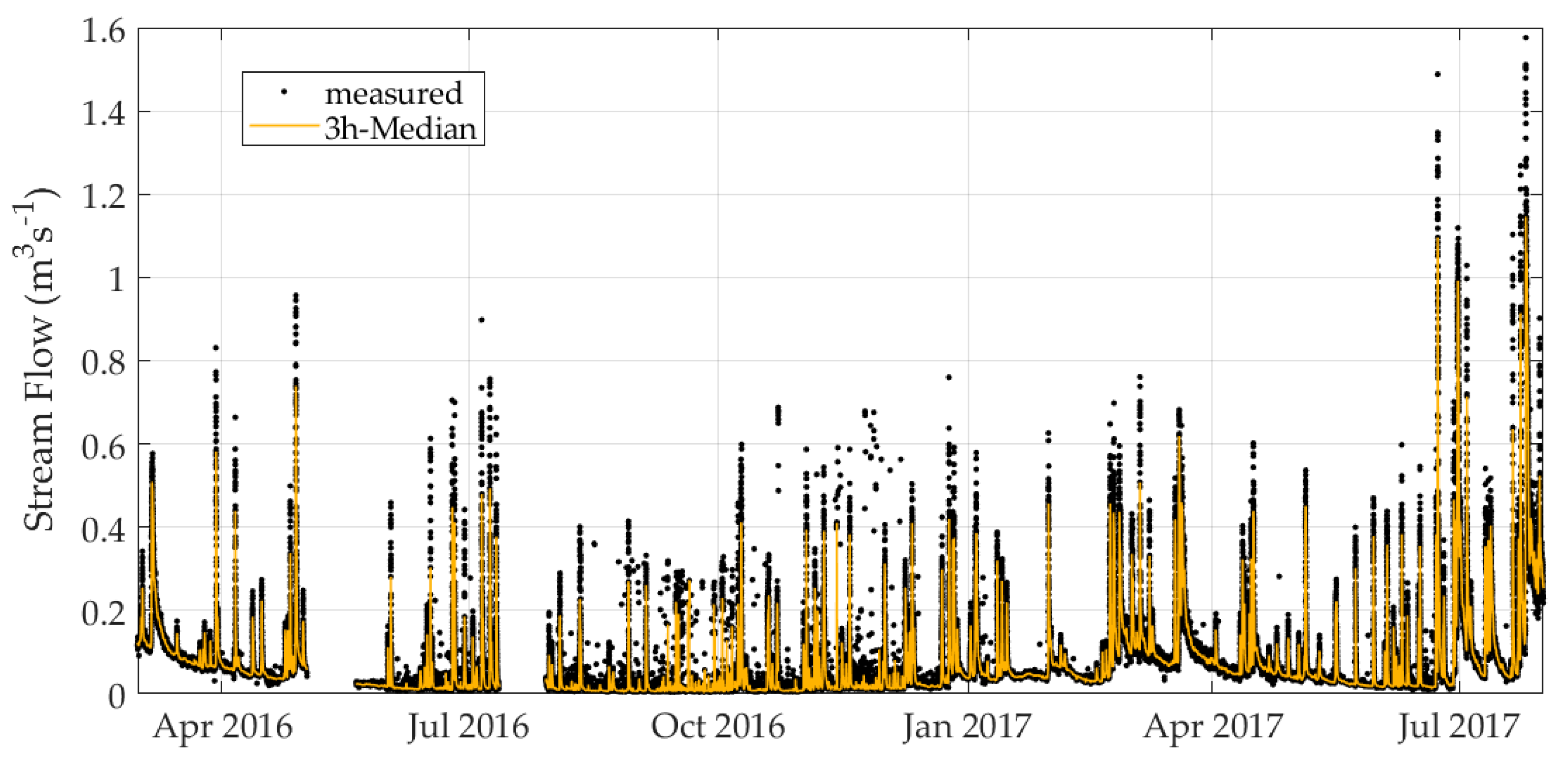
2.1. Study Area and Monitoring Station
2.2. Software Description
2.2.1. SWMM
- ;
- ;
- ;
- ;
- ;
- ;
- ;
- ;
- ; and
- .
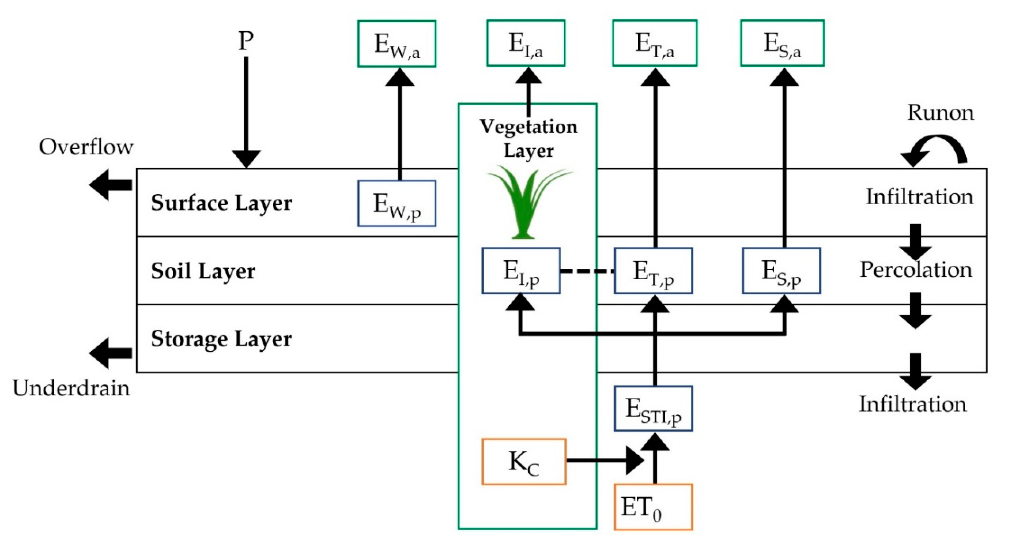
2.2.2. SWMM-UrbanEVA
- ;
- ;
- ; and
- .
- ; and
- .
- ;
- ;
- [11];
- ;
- ; and
- .
- ; and
- .
- ;
- ;
- ; and
- .
- ; and
- .
2.3. Model Setup
2.4. Calibration and Error Measures
3. Results and Discussion
3.1. Sensitivity Analyses
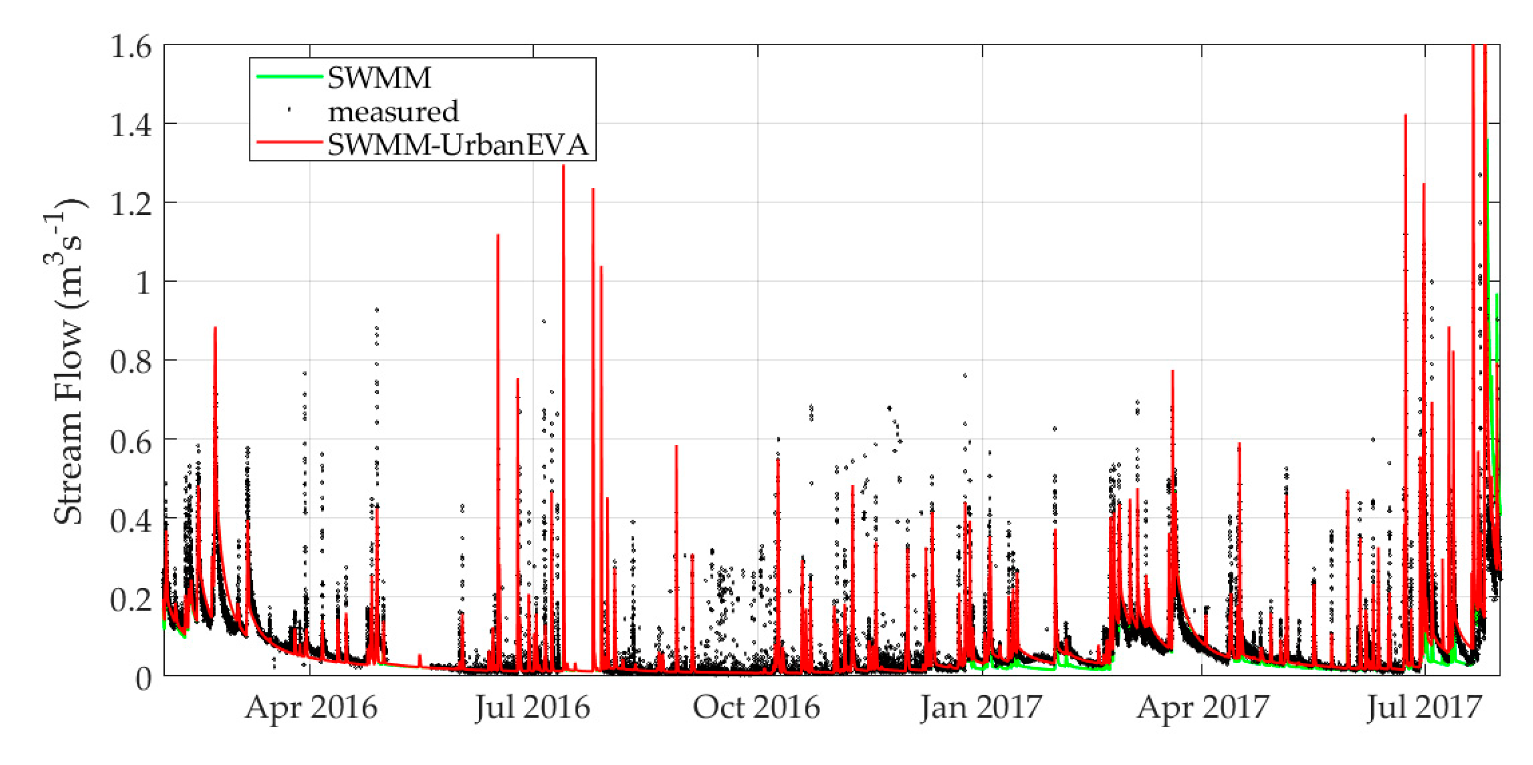
3.2. Calibration Results
3.3. Water Balance
3.4. Groundwater Table and Groundwater Flows to Stream
3.5. Base Flow Separation
- P1: 1 December 2016–20 February 2017Transition phase from low to high base flows; SWMM-UrbanEVA base flows adapt very good to the measured ones, while those produced with SWMM are basically too low. Here, the evaporation in SWMM is too high since leaf fall cannot be incorporated in SWMM.
- P2: 20 February 2017–19 March 2017Phase of high base flows; SWMM-UrbanEVA base flows are higher than the observed ones while those generated with SWMM fit well. Here, the discrepancy can be explained by two possible reasons: According to [13], the crop factor is not constant but changes in dependence of three developmental stages with specific water demands: an initial start-up phase, an intermediate phase in which the highest crop factors (or crop coefficients) are recorded, and a final phase in which the factor decreases again. If this could be taken into account in SWMM-UrbanEVA, it would be possible to calibrate the model, especially the aquifer, differently to achieve an even better adaptation. Another reason could be incorrect leaf area indices, as these were derived from satellite data and this indirect measuring method can lead to underestimation; only spectral data are evaluated and leaves lying on top of each other might not be considered. Besides, the spatial resolution is rather low.
- P3: 19 March 2017–31 May 2017Very high base flows at the beginning of the period caused by voluminous precipitation and exhausted storage capacities in the soil layer. The subsequent emptying of the storage systems is basically reproduced well by both models, but the SWMM-UrbanEVA base flows react more dynamically and therefore adapt a little better.
- P4: 1 July 2017–20 July 2017In this summer month, base flows are above average, due to the relatively humid previous month of June and the subsequent heavy rainfall events in July. At the same time, July is the month with the highest recorded leaf area indices.In the SWMM-UrbanEVA model, GW drainage systems start to operate as early as 1 July, in contrast to the SWMM model, which starts later. This results in a better adapted course of the SWMM-UrbanEVA base flow compared to the measured data.
- P5: 20 July 2017–31 July 2017In the last third of the month, in addition to the high pre-humidity, very strong rainfall occurs, which causes the GW level to rise and restart all drainage systems. In this phase, the largest deviations between SWMM-UrbanEVA and SWMM are registered. The SWMM base flows are extraordinarily high and therefore do not offer a realistic curve. The SWMM-UrbanEVA hydrograph adapts much better, but the peak value of the base flow is still too high during this period. This is probably due to wooded areas, which provide too high peak flows (see Table 8).
4. Conclusions
Author Contributions
Funding
Acknowledgments
Conflicts of Interest
References
- Rossman, L. Storm Water Management Model: User’s Manual Version 5.1. EPA/600/R-14/413 (NTIS EPA/600/R-14/413b). Available online: https://www.epa.gov/sites/production/files/2019-02/documents/epaswmm5_1_manual_master_8-2-15.pdf (accessed on 29 June 2020).
- Hydrologic Engineering Center. Hydrologic Modeling System HEC-HMS Technical Reference Manual; United States Army Corps of Engineers: Washington, DC, USA, 2000. Available online: https://www.hec.usace.army.mil/software/hec-hms/documentation/HECHMS_Technical%20Reference%20Manual_(CPD-74B).pdf (accessed on 26 October 2020).
- Moynihan, K.; Vasconcelos, J. SWMM modeling of a rural watershed in the lower coastal plains of the United States. J. Water Manag. Model. 2014. [Google Scholar] [CrossRef]
- Davis, J.P.; Rohrer, C.A.; Roesner, L.A. Calibration of rural watershed models in the North Carolina Piedmont Ecoregion. In Proceedings of the World Environmental and Water Resources Congress 2007; Available online: https://ascelibrary.org/doi/10.1061/40927%28243%29574 (accessed on 22 October 2020).
- Talbot, M.; McGuire, O.; Olivier, C.; Fleming, R. Parameterization and application of agricultural best management practices in a rural Ontario watershed using PCSWMM. J. Water Manag. Model. 2016. [Google Scholar] [CrossRef]
- Pretorius, H.; James, W.; Smit, J. A Strategy for managing deficiencies of SWMM modeling for large undeveloped semi-arid watersheds. J. Water Manag. Model. 2013. [Google Scholar] [CrossRef]
- Tsai, L.-Y.; Chen, C.-F.; Fan, C.-H.; Lin, J.-Y. Using the HSPF and SWMM Models in a High Pervious Watershed and Estimating Their Parameter Sensitivity. Water 2017, 9, 780. [Google Scholar] [CrossRef]
- Tu, M.-C.; Wadzuk, B.; Traver, R. Methodology to simulate unsaturated zone hydrology in storm water management model (SWMM) for green infrastructure design and evaluation. PLoS ONE 2020, 15, e0235528. [Google Scholar] [CrossRef] [PubMed]
- Feng, Y.; Burian, S. Improving evapotranspiration mechanisms in the U.S. Environmental Protection Agency’s storm water management model. J. Hydrol. Eng. 2016, 21, 6016007. [Google Scholar] [CrossRef]
- Hörnschemeyer, B.; Henrichs, M.; Uhl, M. Setting up a SWMM-integrated model for the evapotranspiration of urban vegetation. In Proceedings of the NOVATECH Lyon 2019, Lyon, France, 1–5 July 2019; pp. 1–4. [Google Scholar]
- Hörnschemeyer, B. Modellierung der Verdunstung Urbaner Vegetation: Weiterentwicklung des LID-Bausteins im US EPA Storm Water Management Model; Springer Spektrum: Berlin, Germany, 2019; p. 197. [Google Scholar]
- Hörnschemeyer, B.; Henrichs, M.; Uhl, M. Ein SWMM-Baustein für die Berechnung der Evapotranspiration von urbaner Vegetation. In Proceedings of the Aqua Urbanica 2019: Regenwasser Weiterdenken—Bemessen trifft Gestalten, Rigi Kaltbad, Switzerland, 8–10 September 2019; pp. 133–140. [Google Scholar]
- Allan, R.; Pereira, L.; Raes, D.; Smith, M. FAO Irrigation and Drainage Paper No. 56. Available online: http://www.fao.org/3/X0490E/x0490e00.htm (accessed on 24 September 2020).
- Hydrologischer Atlas Deutschland. Teil 2: Hydrometeorologie; Bundesamt für Gewässerkunde (BfG). Available online: https://geoportal.bafg.de/mapapps/resources/apps/HAD/index.html?lang=de (accessed on 24 September 2020).
- Pettyjohn, W.A.; Henning, R. Preliminary estimate of ground-water recharge rates, related streamflow and water quality in Ohio: Ohio State University Water Resources Center Project Completion; The Ohio State University: Columbus, OH, USA, 1979. [Google Scholar]
- Rossman, L.; Huber, W. Storm Water Management Model: Reference Manual Volume I—Hydrology (Revised). EPA/600/R-15/162A. Available online: https://nepis.epa.gov/Exe/ZyPDF.cgi/P100NYRA.PDF?Dockey=P100NYRA.PDF (accessed on 24 September 2020).
- Hossain, S.; Hewa, G.A.; Wella-Hewage, S. A Comparison of continuous and event-based rainfall–runoff (RR) modelling using EPA-SWMM. Water 2019, 11, 611. [Google Scholar] [CrossRef]
- Rossman, L. Storm Water Management Model: Reference Manual Volume II—Hydraulics. EPA/600/R-17/111. Available online: https://nepis.epa.gov/Exe/ZyPDF.cgi?Dockey=P100S9AS.pdf (accessed on 24 September 2020).
- Bremicker, M. Aufbau eines Wasserhaushaltsmodells für das Weser-und das Ostsee-Einzugsgebiet als Baustein Eines Atmosphären-Hydrologie-Modells. Ph.D. Thesis, Albert-Ludwigs-Universität Freiburg, Freiburg, Germany, 1998. [Google Scholar]
- Bremicker, M. Das Wasserhaushaltsmodell LARSIM: Modellgrundlagen und Anwendungsbeispiele. Freibg. Schr. Hydrol. 2000, 11, 1–130. [Google Scholar]
- Braden, H. Ein Energiehaushalts- und Verdunstungsmodell für Wasser und Stoffhaushaltsuntersuchungen landwirtschaftlich genutzter Einzugsgebiete. Mitt. Dtsch. Bodenkd. Ges. 1985, 42, 294–299. [Google Scholar]
- Deardorff, J.W. Efficient prediction of ground surface temperature and moisture, with inclusion of a layer of vegetation. J. Geophys. Res. 1978, 83, 1889–1903. [Google Scholar] [CrossRef]
- Dickinson, R.E. Modeling Evapotranspiration for Three-Dimensional Global Climate Models; Geophysical Monograph Series; AGU Publishing: Washington, DC, USA, 1984; ISBN 9781118666036. [Google Scholar] [CrossRef]
- Kroes, J.G.; van Dam, J.C.; Groenendijk, P.; Hendriks, R.F.A.; Jacobs, C.M.J. SWAP Version 3.2–Theory Description and User Manual; Alterra Wageningen: Wageningen, The Netherlands, 2008. [Google Scholar]
- Schulla, J. Model Description WaSiM (Water Balance Simulation Model); Hydrology Software Consulting: Zürich, Switzerland, 2012. [Google Scholar]
- Madsen, H. Automatic calibration of a conceptual rainfall–runoff model using multiple objectives. J. Hydrol. 2000, 235, 276–288. [Google Scholar] [CrossRef]
- Barco, J.; Wong, K.M.; Stenstrom, M.K. Automatic Calibration of the U.S. EPA SWMM Model for a Large Urban Catchment. J. Hydraul. Eng. 2008, 134, 466–474. [Google Scholar] [CrossRef]
- Krause, P.; Boyle, D.; Bäse, F. Comparison of different efficiency criteria for hydrological model assessment. Adv. Geosci. 2005, 5, 89–97. [Google Scholar] [CrossRef]
- Chiew, F.H.; McMahon, T.A. Assessing the adequacy of catchment streamflow yield estimates. Aust. J. Soil Res. 1993, 31, 665–680. [Google Scholar] [CrossRef]
- Moriasi, D.; Gitau, M.; Pai, N.; Daggupati, P. Hydrologic and water quality models: Performance measures and evaluation criteria. Trans. ASABE 2015, 58, 1763–1785. [Google Scholar] [CrossRef]
- Zenker, T. Verdunstungswiderstände und Gras-Referenzverdunstung: Lysimeteruntersuchungen zum Penman-Monteith-Ansatz im Berliner Raum. Ph.D. Thesis, Technische Universität Berlin, ehemalige Fakultät VII—Architektur Umwelt Gesellschaft, Berlin, Germany, January 2003. [Google Scholar]


| Land Use Class | Abbreviation | Area Fraction (%) | Thereof Sealed (%) |
|---|---|---|---|
| agriculture | AC | 29.2 | 0 |
| wetland | WL | 0.1 | 0 |
| grassland | GL | 1.3 | 0 |
| industry/trade | IT | 5.0 | 62.5 |
| deciduous forest | DF | 0.3 | 0 |
| mixed forest | MF | 6.0 | 0 |
| coniferous forest | CF | 1.3 | 0 |
| orchard | OR | 11.5 | 0 |
| residential area | RA | 17.8 | 49.4 |
| parks | PA | 15.3 | 26.7 |
| traffic area | TA | 11.0 | 51.0 |
| water surface | WA | 1.2 | 0 |
| Designation | Abbreviated Designation | Formula | No. |
|---|---|---|---|
| Volume Error | EVol | (25) | |
| Mean absolute Error | MAE | (26) | |
| Correlation Coefficient | R | (27) | |
| Nash Sutcliffe Efficiency | NSE | (28) |
| Very Good | Good | Satisfactory | Not Satisfactory | Source | |
|---|---|---|---|---|---|
| R | R ≥ 0.93 | 0.8 ≤ R < 0.93 | 0.6 ≤ R < 0.8 | R < 0.6 | [29] |
| NSE | >0.80 | 0.60 ≤ NSE ≤ 0.80 | 0.50 < NSE < 0.60 | ≤0.50 | [30] |
| Parameter | Unit | Calibrated Value, Range, or Calculation Formula | Sensitivity to Stream Flow | Effects of Parameter Changes/Comment |
|---|---|---|---|---|
| Subcatchment Characteristics | ||||
| Width | m | medium | The greater the width of the subcatchments, the shorter the flow path, the earlier and larger the direct peak runoff | |
| Manning value impervious | s (m1/3)−1 | 0.05 | medium | large values slow down surface runoff and reduce peak flow |
| Detention storage impervious | mm | 0.5 | medium | Cuts peak runoff; small rain events are “swallowed” if value is too high |
| LID Control | ||||
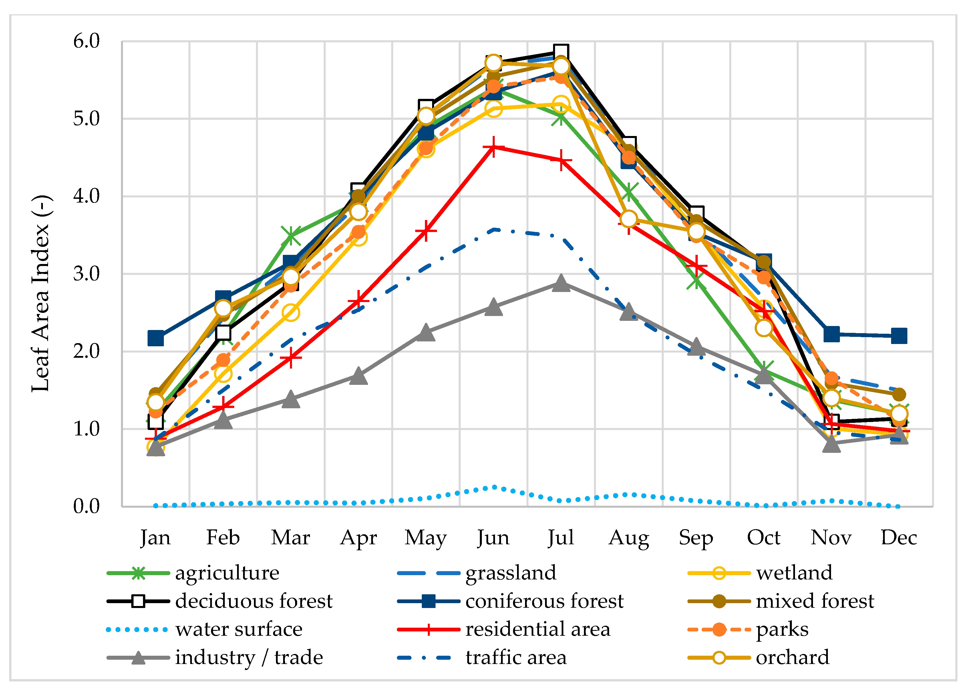
| average LAI * | m m−1 | 1.7–3.6 | medium | The higher the value, the more ET, the less GW base flow in the stream |
| LAI monthly coefficients * (pattern) | - | 0.2–1.7 | medium | increases seasonal dynamics of actual ET throughout the year; Increased ET in summer leads to lower GW levels and therefore less GW inflow to stream |
| crop factor * (KC) | - | 0.7–1.5 | high | The higher the value, the more ET, the lower the GW level, the less GW base flow in the stream |
| Groundwater (Physical Parameters) | ||||
| Porosity | - | 0.43 | high | Increasing the value causes delay of GW peak discharge; more extreme course of the base flows in the stream (high flows higher, lower flows lower) |
| Conductivity Slope | - | 18 | medium | the higher the value, the later the lateral GW discharges react (delay of GW peak flows) |
| Upper Evaporation Fraction | - | 0.1 | high | the lower the value, the higher the base flow in average; positive correlation with lower GW loss rate |
| Lower GW Loss Rate (Seep) | mmh−1 | 5.0 × 10⁻⁶ | high | the lower the value, the higher the base flow in average |
| Groundwater Flow Editor | ||||
| A1 | - | 0.04 (0.0003 for sealed areas) | high | The smaller the value, the flatter/slower the flows decrease, making base flows higher |
| B1 | - | 2 | high | The smaller the value, the larger the peaks, less base runoff |
| A2 and A3 B2 | - | 0 1 | high | Level of surface water does not significantly affect GW flow; by setting the coefficients to zero and B2 to 1, it is excluded from the power function |
| Threshold Water Table Elevation | m | 1.2 m below surface height | high | the lower the threshold, the higher the lateral GW discharges to the stream |
| Land Use Class | Crop Factor KC (-) |
|---|---|
| agriculture | 1.5 |
| wetland | 1.3 |
| grassland | 1.3 |
| industry/trade | 0.7 |
| deciduous forest | 0.8 |
| mixed forest | 0.8 |
| coniferous forest | 0.8 |
| orchard | 1 |
| residential area | 0.7 |
| parks | 1.3 |
| traffic area | 0.7 |
| water surface | 0.7 |
| E_Vol (%) | MAE (m3s−1) | R (-) | NSE (-) | |
|---|---|---|---|---|
| SWMM | 10.4 | 0.032 | 0.80 | 0.44 |
| SWMM-UrbanEVA | 3.6 | 0.026 | 0.82 | 0.68 |
| SWMM-UrbanEVA | SWMM | |
|---|---|---|
| Runoff Quantity | Depth (mm) | Depth (mm) |
| Total Precipitation | 1162 | 1162 |
| Evaporation Loss | 666 | 715 |
| Infiltration Loss | 373 | 324 |
| Surface Runoff | 95 | 95 |
| Groundwater | Depth (mm) | Depth (mm) |
| Infiltration | 373 | 324 |
| GW Flow | 388 | 368 |
| Flow Routing | Volume (106 L) | Volume (106 L) |
| Wet Weather Inflow | 2144 | 2144 |
| GW Inflow | 8771 | 8302 |
| MAE (m3s−1) | R (-) | NSE (-) | |
|---|---|---|---|
| SWMM | 0.014 | 0.88 | 0.81 |
| SWMM-UrbanEVA | 0.011 | 0.93 | 0.85 |
Publisher’s Note: MDPI stays neutral with regard to jurisdictional claims in published maps and institutional affiliations. |
© 2020 by the authors. Licensee MDPI, Basel, Switzerland. This article is an open access article distributed under the terms and conditions of the Creative Commons Attribution (CC BY) license (http://creativecommons.org/licenses/by/4.0/).
Share and Cite
Kachholz, F.; Tränckner, J. Long-Term Modelling of an Agricultural and Urban River Catchment with SWMM Upgraded by the Evapotranspiration Model UrbanEVA. Water 2020, 12, 3089. https://doi.org/10.3390/w12113089
Kachholz F, Tränckner J. Long-Term Modelling of an Agricultural and Urban River Catchment with SWMM Upgraded by the Evapotranspiration Model UrbanEVA. Water. 2020; 12(11):3089. https://doi.org/10.3390/w12113089
Chicago/Turabian StyleKachholz, Frauke, and Jens Tränckner. 2020. "Long-Term Modelling of an Agricultural and Urban River Catchment with SWMM Upgraded by the Evapotranspiration Model UrbanEVA" Water 12, no. 11: 3089. https://doi.org/10.3390/w12113089
APA StyleKachholz, F., & Tränckner, J. (2020). Long-Term Modelling of an Agricultural and Urban River Catchment with SWMM Upgraded by the Evapotranspiration Model UrbanEVA. Water, 12(11), 3089. https://doi.org/10.3390/w12113089